Landscape Pattern Consistency Assessment of 10 m Land Cover Products in Different Ecological Zoning Contexts of Sichuan Province, China

Abstract

The research on land cover and its changing value to the ecology environment and ecosystem service is of great importance. Understanding the landscape patterns and accuracy in remote sensing land cover data from multiple sources under eco-regionalization is important for relevant research under eco-regionalization. Land cover and land use in different ecological regionalization contexts influence massive ecosystem processes on a global scale, and many ecosystem models are dependent on accurate land cover information. It is, therefore, important to assess the available global land cover products based on different ecological zoning contexts and to understand the differences between them so that different researchers can apply them in a rational way. This study took Sichuan Province as an experimental case. Based on the three methods of spatial superposition, landscape index, and validation sample, we discussed and then analyzed the consistency of landscape patterns for the three 10 m global land cover data under different ecogeographic zones. The results showed that the spatial consistency of FROM-GLC, ESA, and ESRI land cover data were high under the ecological zoning of Palearctic0518 (PA0518) and PA1017, while the spatial pattern was less consistent for the three land cover data under the ecological zoning of PA0509 and PA0437. The fully consistent areas for the three data were 44,420.9 km² and 53,368.9 km², respectively. The results of the quantitative analysis of the landscape index showed significant differences in the degree of landscape fragmentation, landscape shape complexity, and the connectivity among landscape patches of several land cover data were significantly different under different ecological zones. Based on the three kinds of independent validation samples to achieve the absolute accuracy of evaluation, the overall accuracy of the FROM-GLC, ESA, and ESRI land cover data was less than 60%, and future drawing still needs to further improve the regional land cover data mapping accuracy under different ecological zones in order to carry out ecological environment monitoring, land ecological security evaluation, and related research to provide a reference.

1. Introduction

Land cover and land use in different ecological regionalization contexts influence ecosystem processes at a large scale on the global scale, and a number of Earth system models depend on accurate land cover information. The study of the land cover landscape patterns and their continuous transformation is an effective means of revealing regional ecological conditions and spatial changes. Land cover is also an important factor reflecting the surface solar radiation energy [1], and its spatial pattern distribution and dynamic change are closely related to species diversity, agricultural development, and ecological protection, among others. It is crucial in the material cycle, the energy cycle, and the sustainability of surface resources [2,3,4,5,6].

The rapid advances in remote sensing technology have promoted the use of aerospace data for land surface mapping. At present, a large number of land cover product data are now publicly available [7], for instance, the International Geosphere-Biosphere Programme Data and Information System Cover (IGBP DISCover) data [8], Global Land Cover 2000 (GLC2000) data [9], and GlobeLand30 data [10]. The production from these land cover data supports data for global and regional ecosystem inversion, land-surface process simulation, agriculture, and other related studies [11,12,13,14]. Nevertheless, because of the diversity of sources of data and methodologies of classification, it is difficult to keep these remote sensing from multiple sources of land cover data consistent [15,16,17]. The differences among multiple sources of remote sensing data are mainly reflected in the number and spatial morphological distribution of surface cover, exposing users to unpredictable uncertainty when using specific land cover data to fulfill their business needs, especially the medium- and high-resolution land cover data released publicly [18,19]. However, how to select appropriate land cover data and to what extent the selected data can meet the research needs of users are challenges faced by land cover users.

The performed studies at home and abroad have evaluated and analyzed the free remote sensing land cover data [20,21]. For instance, Giri et al. [22] used common methods of area comparison and spatial consistency analysis to make a full-scale comparative analysis of GLC2000 and MODIS land cover products with coarse resolution. The experiments revealed that the spatial patterns for the two land cover data were less consistent under the fine type, and the percentage consistency between the two data sets also varied greatly between biomes. Giri’s comparative analytical offers insights for both data producers and users. Yang et al. [23] assessed and analyzed seven land cover products (IGBP DISCover, UMD, GLC, MCD12Q1, GLCNMO, CCI-LC, and GlobeLand30) by using area comparison, spatial pattern comparison, and accuracy evaluation based on verification points. The results show that the GLC 2000 and CCI-LC 2000 have a high spatial agreement, with a percentage of 53.8% of the agreement region. In addition, the accuracy of the seven kinds of data was higher in the homogenous region and lower in other areas. Chen et al. [24] evaluated and analyzed four global land cover data (MODIS, GlobCover2009, FROM-GC, and GlobeLand30) for cropland types. The experimental results indicate that the total accuracy of the four data types are between 61.26% and 80.63%, and the classification accuracy of the cropland type in GlobeLand30 is the highest. Chen’s research can provide a reference value for building a fusion of cropland classification datasets. Kang et al. [25] assessed the consistency of three 30 m spatial resolution land cover data from northern Laos based on the landscape index method. The experimental results show that the three data differ significantly in terms of landscape indices and spatial pattern distribution. Taking the Arctic as the experimental area, Liang et al. [26] assessed data from four global land cover products (CCI-LC, GLCNMO, MODIS, and GlobeLand30) covering the Arctic region and experimentally found that MODIS data had the lowest overall accuracy of 29.5%. Existing research on the assessment and analysis of various land cover products provides a useful reference value for land cover producers and users.

However, there are few landscape pattern evaluations of high-resolution land cover data in various ecological zones [27]. In fact, the mapping accuracy of some complex landscape cover types is low. The ecological geographic area is in accordance with the natural geographical variation of the division or merger of different levels of regional systems; therefore, from the perspective of ecological geographical division to evaluate multi-source remote sensing land cover data analysis, in terms of ecosystem service benefits of land use, biodiversity and the regional ecological environment effects of research is very important. However, through the literature review, there has been no evaluation study on the consistency of landscape patterns of global 10 m land cover data in different ecological zones. However, through the literature review [28,29,30], there are few studies on the consistent estimation and analysis of landscape patterns of high-resolution (10 m) global land cover data under different ecological zones.

Therefore, the three global land cover product data, FROM-GLC, ESA, and ESRI, were selected as the study data for this paper, using Sichuan Province, China as the study area. The consistency of landscape patterns under various ecological zones was evaluated by a process of spatial overlay, landscape index, and accuracy of the three independent validation samples, and the factors affecting data inconsistency were discussed. The experimental results can provide a reference value for the research of ecological environment monitoring, ecosystem service function, and land resources sustainable development.

2. Study Area and Data

2.1. Study Area

Sichuan Province in Southwest China (Figure 1), bounded between latitude 26°03′–34°19′ N and longitude 97°21′–108°12′ E. It also shares borders with the Chinese provinces of Chongqing, Guizhou, Yunnan, Tibet Autonomous Region, Qinghai, Gansu, and Shaanxi. The topography of Sichuan varies considerably from east to west and is complex, with four topographic types of mountains hills, plains, and plateaus. It spans the different landform units of the Tibetan Plateau, the Hengduan Mountains, the Yunnan-Guizhou Plateau, the Qinba Mountains, and the Sichuan Basin. The regional distribution of light and hot water is extremely uneven in Sichuan Province. Sichuan Province is in a transitional zone at the central and lower regions of the Qinghai-Tibet Plateau and the Yangtze River plain, with a wide range of high and low levels, especially in the western and eastern regions. The central western part of Sichuan Province is a plateau and mountain, with an altitude of more than 3000 m, and the eastern is a basin and hilly, with an altitude of 500–2000 m. Sichuan Province is classified into three climates, namely the Sichuan Basin subtropical humid climate, the subtropical subhumid climate of mountainous southwest Sichuan Province, and the alpine and plateau alpine cold climate of northwest Sichuan Province. The overall climate is pleasant. Sichuan Province has many rivers, mainly the Yangtze River system, and the main lakes are Qionghai Lake, Lugu Lake, and Ma Lake. Sichuan Province has a wide range of mineral resources, including energy, non-ferrous and rare precious metals. As the most intuitive representation of the regional ecological environment and ecosystem, it is vital to have current and reliable information on land cover in Sichuan Province.

2.2. Study Data

(1) Land cover product data. Three 10 m worldwide land cover product data were used for the consistency analysis of landscape patterns under different ecological zones in this paper. The three land cover data are FROM-GLC [31] (http://data.ess.tsinghua.edu.cn./ (accessed on 18 January 2022)), produced by Tsinghua University, ESA (https://zenodo.org/record/5571936), produced by the European Space Agency, and ESRI [32] (https://www.arcgis.com/index.html), produced by Environmental Systems Research Institute (

Table 1. The main parameter information of three kinds of land cover data.

Name	Resolution(m)	Time	Method	Overall Accuracy (%)	Satellite
FROM-GLC	10	2017	Random forest	72.76	Sentinel-2
ESA	10	2020	Deep learning model	74.40	Sentinel-1/2
ESRI	10	2020	Deep learning model	85.96	Sentinel-2

). Existing studies [33] have shown that natural ecosystems may undergo major changes within 10 years. In addition, based on the high-resolution images from Google Earth, surface changes in the study area during 2017–2020 were minimal. Therefore, the errors due to temporal differences in the three land cover data are small enough to meet the research requirements of the paper.

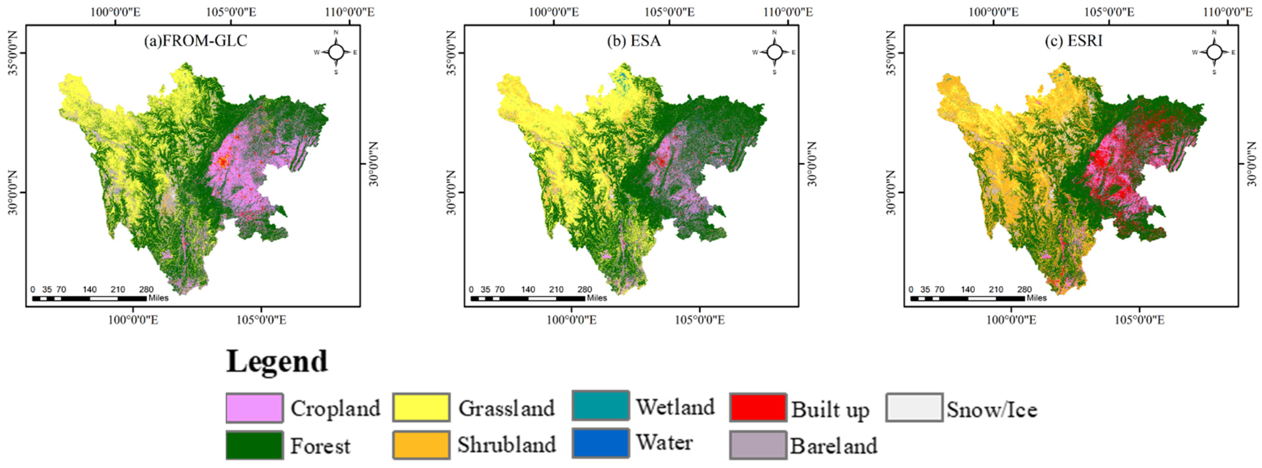
The three types of global land cover product data need to be processed first when conducting a landscape pattern consistency analysis. Firstly, the three kinds of data were cropped to the borderline in the study area. The projections and coordinate systems of the three data were then converted to UTM and WGS84. Finally, according to the existing research [34,35] and the definition of moss and lichen, in this study, the tundra present in the FROM-GLC product and the moss and lichen species present in the ESA product were combined into a single shrubland.

Table 2. The three original classification systems of land cover data and their correspondence.

Merged	Code	FROM-GLC	Code	ESA	Code	ESRI
Cropland	10	Cropland	40	Cropland	5	Crops
Forest	20	Forest	10	Tree cover	2	Trees
Grassland	30	Grassland	30	Grassland	3	Grass
Shrubland	40	Shrubland	20	Shrubland	6	Shrubs
	70	Tundra	100	Moss and lichen
Wetland	50	Wetland	90	Herbaceous wetland	4	Flooded vegetation
			95	Mangroves
Water	60	Water	80	Permanent water bodies	1	Water
Built-up	80	Impervious surface	50	Built-up	7	Built area
Bare land	90	Bare land	60	Bare/sparse vegetation	8	Bare ground
Snow/Ice	100	Snow/Ice	70	Snow and ice	9	Snow/Ice

shows the classification system. Figure 2 illustrates the three data spatial distributions.

(2) Terrestrial Ecoregions of the World (TEOW) data (https://www.worldwildlife.org/publications/terrestrial-ecoregions-of-the-world, (accessed on 15 January 2022)). The TEOW data are based on a biogeographic delineation of terrestrial biodiversity. TEOW contains 867 ecoregions, which are based on 14 biomes (such as forest, grassland, etc.,) and 8 biogeographic zones [36]. TEOW data provide a sound scientific basis for understanding and mastering global ecological resources and protecting biodiversity. Figure 3 and

Table 3. The code and name of each terrestrial ecological zone.

Code	Name
PA1017	Southeast Tibet shrublands and meadows
PA1020	Tibetan Plateau alpine shrublands and meadows
PA0509	Hengduan Mountains subalpine conifer forests
PA0516	Nujiang Langcang Gorge alpine conifer and mixed forests
PA0518	Qionglai-Minshan conifer forests
PA0101	Guizhou Plateau broadleaf and mixed forests
PA0102	Yunnan Plateau subtropical evergreen forests
PA0417	Daba Mountains evergreen forests
PA0434	Qin Ling Mountains deciduous forests
PA0437	Sichuan Basin evergreen broadleaf forests

indicate the position and the name of the terrestrial ecoregions, respectively.

3. Methods

3.1. Consistency of the Spatial Pattern

In this study, the spatial overlay method was used to directly represent the differences in the spatial pattern of the three land cover data in different ecological zones. First, the minimum unit is the spatial resolution (10 m) of the three selected data. Then, the grid calculator in the ArcGIS tool is used to calculate the pixel-by-pixel spatial correspondence of the three types of data. Finally, count the number of different data matching coverage types by pixel and divide the spatial consistency results into three levels, as follows. (1) Completely inconsistent; the types of land cover data displayed on a certain raster point are not the same. (2) Basically consistent; any two of the three types of data display the same type on a grid point. (3) Completely consistent; the types of land cover data displayed on a certain grid point were all the same. Figure 4 is a schematic diagram of space superimposed (taking cropland type as an example).

3.2. Landscape Pattern Analysis

In landscape ecology, the landscape index can be used to quantitatively describe and analyze landscape patterns [37]. The complexity of the regional landscape and the correlation between landscape indexes are certain. Some relevant landscape indexes are used in the study of landscape patterns, which will affect the reflection of spatial heterogeneity and diverse characteristics of the landscape. Therefore, based on the ecological significance represented by different landscape indexes, and according to the relevant research [38] and the selected characteristics of the study area, this paper finally selects PD (representing landscape heterogeneity), LSI (representing shape complexity), and AI (representing landscape connectivity) as the landscape indexes for this study. The definitions and ecological meanings of the three indices selected are as follows.

(1)

The PD landscape index mainly describes landscape fragmentation and, at the same, time reflects the heterogeneity of the landscape. The calculation formula is:

$$PD=\frac{N}{A}, PD>0$$

(1)

where N is the total patch number and A is the total landscape area.

(2)

LSI is used to represent the landscape shape characteristics. The LSI value is closer to 1 when the landscape shape is simpler. The calculation formula is:

$$LSI=\frac{0.25E}{\sqrt{A}}, LSI\ge 1$$

(2)

where E is the total length of all plaques and A is the total area.

(3)

AI is mainly used to describe the connectivity between patches. When the AI value is smaller, the patches are more discrete. The calculation formula is:

$$AI=\left[\frac{g_{ii}}{\max g_{ii}}\right]\times 100, 0\le AI\le 100$$

(3)

where $g_{ii}$ is the number of analog joins between pixels of patch type $i$.

3.3. Accuracy Verification Based on the Three Independent Samples

At present, the commonly used and better accuracy verification method is the confusion matrix based on verification points [39,40,41]. This method can be used to calculate the indexes for estimating the precision of the total and each surface type, including Overall Accuracy (OA), Producer Accuracy (PA), User Accuracy (UA), and Kappa coefficient. The calculation formula is [42]:

$$OA=\frac{{\sum }_{i=1}^r{x}_{ii}}{n}\times 100\%$$

(4)

$$PA=\frac{x_{ii}}{x_{+i}}\times 100\%$$

(5)

$$UA=\frac{x_{ii}}{x_{i+}}\times 100\%$$

(6)

$$Kappa=\frac{N·{\sum }_{i=1}^r{x}_{ii}-{\sum }_{i=1}^r\left(x_{i+}·x_{+i}\right)}{N^2-{\sum }_{i=1}^r\left(x_{i+}·x_{+i}\right)}$$

(7)

where $x_{ii}$ is the number of correctly classified pixels in the $i$ surface type, $n$ is the total pixel number, $x_{i+}$ is the total number of pixels of type $i$ in the estimated data, $x_{+i}$ is the total number of pixels of type $i$ in the reference data, $r$ is the number of rows in the confusion matrix, and $N$ is the total number of samples.

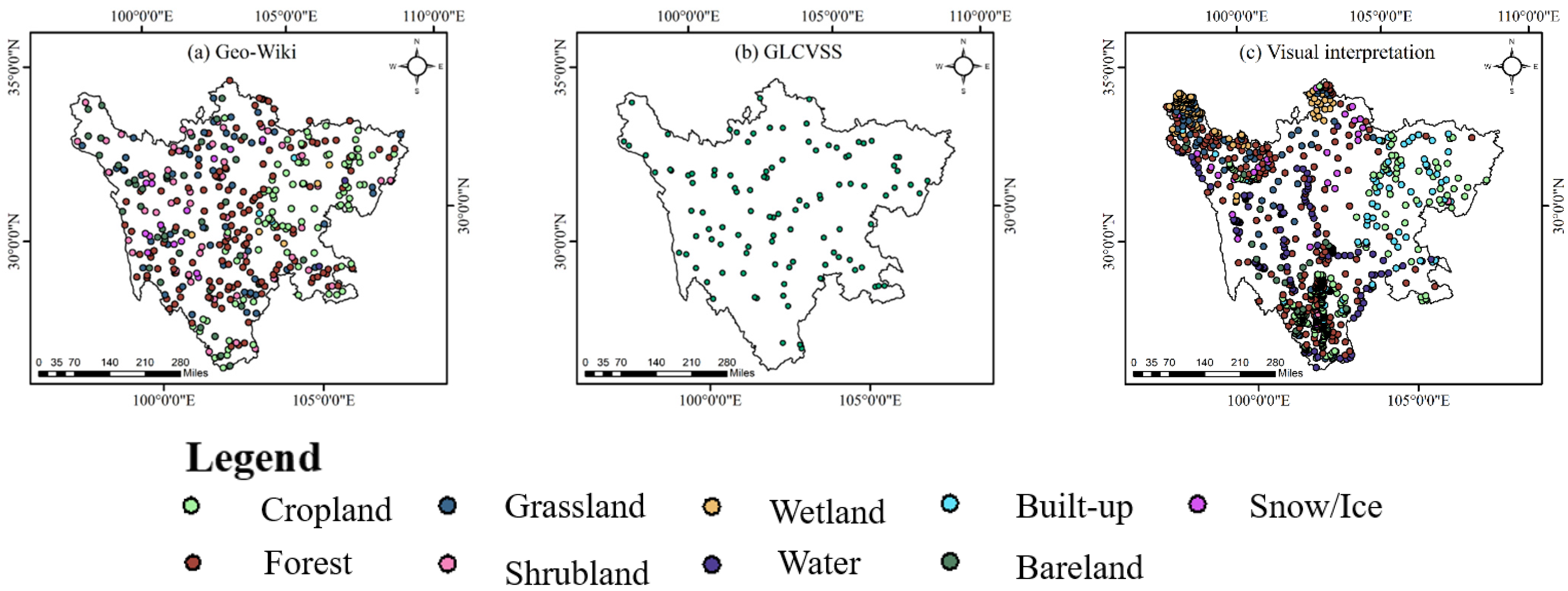
Yang et al. [43] produced a 30 m (1990–2019) land cover dataset CLCD, and used visual interpretation points and two check points to verify the precision of CLCD data. Therefore, to verify the precision of the three data from multiple perspectives, this paper referred to Yang’s article and used three independent verification samples. The three independent validation samples obtained in this paper are (1) The Geo-Wiki [44] samples, and this sample includes 10 types. In this paper, 724 Geo-wiki samples are finally obtained by cutting the boundary line of the area (Figure 5a). (2) The Global Land Cover Validation Sample Set (GLCVSS) [45], a the sample that is distributed evenly in space. Similarly, in this study, 106 GLCVSS samples were finally obtained through the boundary line (Figure 5b). (3) The visual interpretation of the collected samples. So as to decrease the error of position and visual discrimination in the research results, this paper abided by several theories when collecting points. First, the point should be selected as the middle of the homogeneous region of the error range. Second, the time of the Google image at the acquisition point is consistent with the evaluated data. Finally, the final sample was determined after several independent interpretations by several experts. This paper takes Google Earth high-resolution images, Geo-Wiki, and GLCVSS as reference data, and visually interprets 952 samples (Figure 5c).

4. Results

4.1. Spatial Pattern Consistency under TEOW

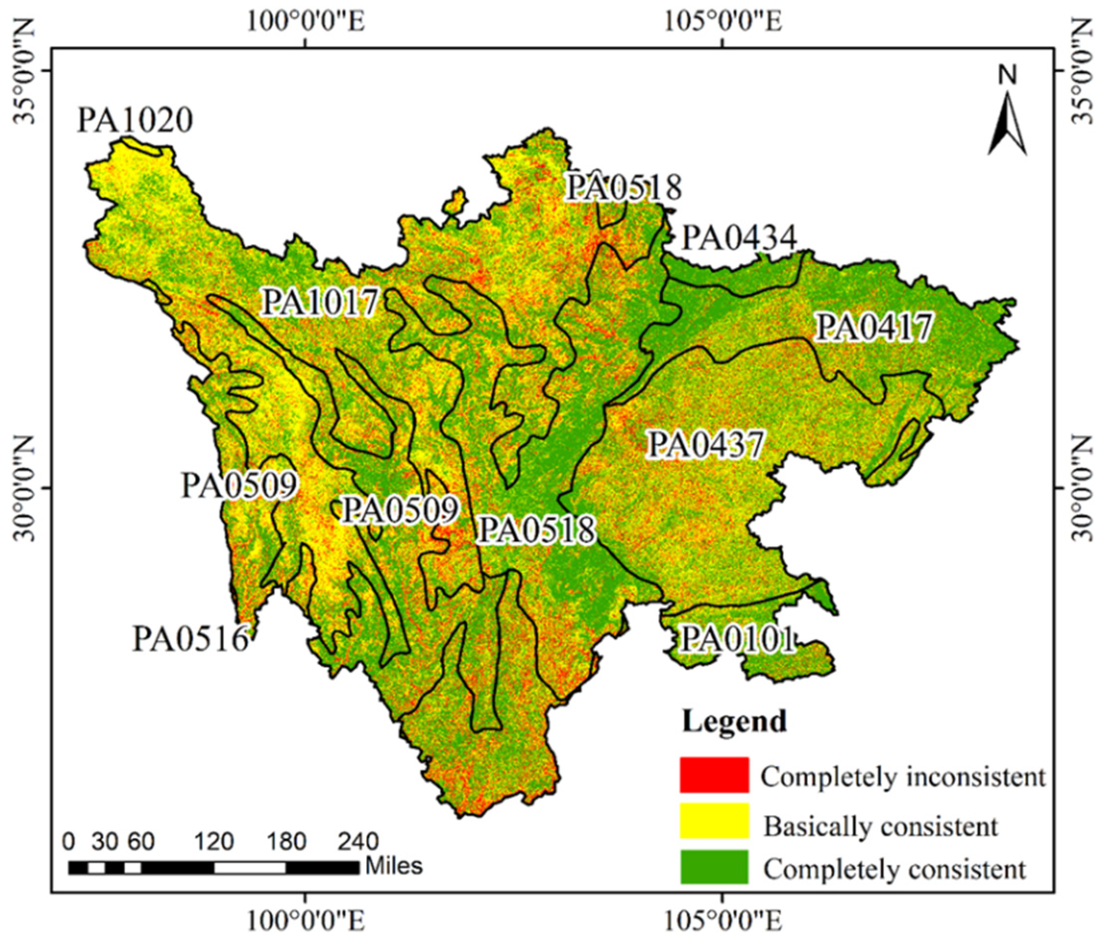
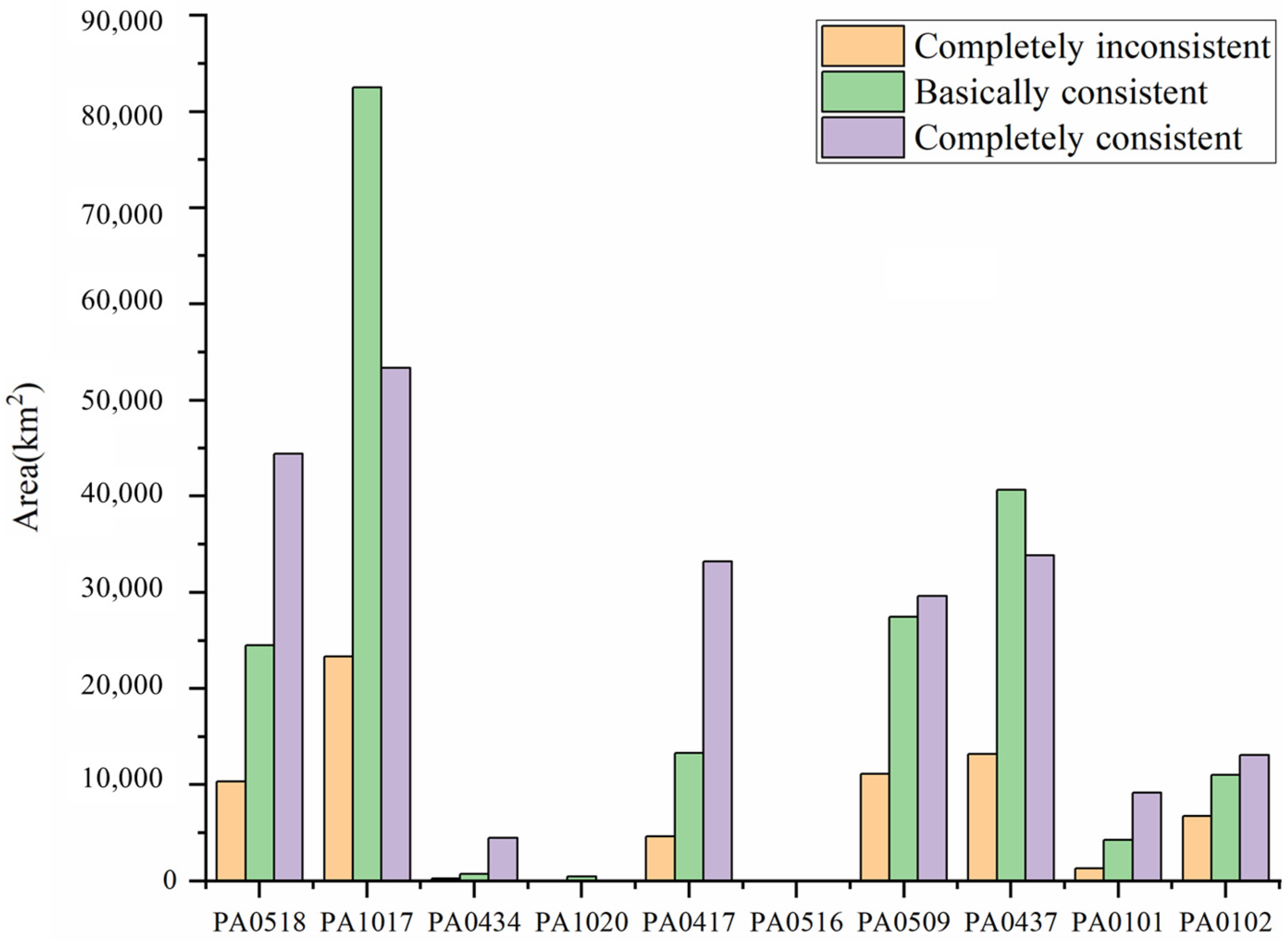
The spatial pattern consistency and area statistics of the three data in the various ecoregions are shown in Figure 6 and Figure 7. The experimental results indicate that the consistency of the three data is high under PA0518 and PA1017 ecological zoning, which was mainly in the central plain of Chengdu and a section of the mountainous zones of northern Sichuan, and these areas were chiefly dominated by forest types. Under the ecological zoning of PA0518 and PA1017, the areas with identical land cover data are 44,420.9 km² and 53,368.9 km², respectively. The three land cover data under PA0509 and PA0437 ecoregions are less consistent, which are situated in the mountainous zones in the south region and parts of the eastern Sichuan Basin, with fully unconformable areas of 11,112.0 km² and 13,215.1 km², respectively. These areas have a complex land cover type, such as staggered distribution of cropland, construction, and grassland. The PA1017 ecoregion is large scale in Sichuan Province, and the spatial inconsistency of the three data under PA1017 was also high; it is found mainly in northern Sichuan Province. The area where the three data do not agree at all is 23,305.9 km².

4.2. Landscape Pattern Consistency under TEOW

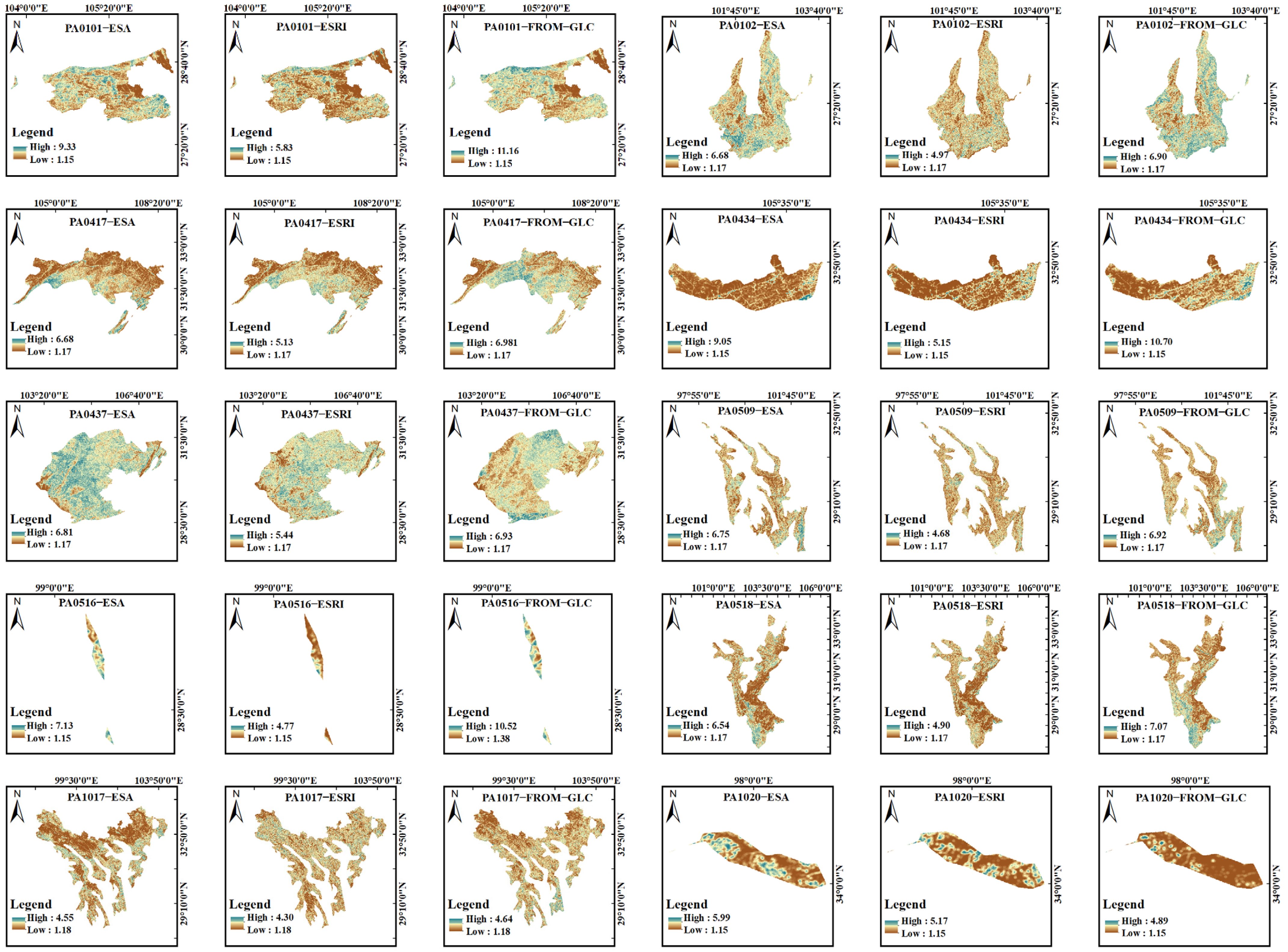
The landscape pattern of PD indices for the three data under different ecoregions is shown in Figure 8. Experimental results show that the spatial pattern distribution of PD indices differs somewhat between the three land cover data, indicating an inconsistency in the surface landscape fragmentation between the three data. Under the ecological zoning of PA0102, PA0509, PA0516, and PA1017, ESA and FROM-GLC land cover data PD indices have a more consistent spatial pattern distribution; that is, the two data reflect a relatively consistent degree of surface landscape fragmentation. Under the ecological zoning of PA0417 and PA0518, ESA and ESRI land cover data have a relatively consistent distribution of PD index spatial patterns; that is, the two data reflect a relatively consistent degree of surface landscape fragmentation. Under the ecological zoning of PA0101, PA0434, PA0437, and PA1020, there was a low spatial pattern distribution of PD indices for the three data; in other words, the surface landscape fragmentation of the three data was quite different.

Figure 9 is the spatial pattern distribution of the LSI index of the three land cover data under different ecoregions. The results of the experiment indicate that there is some variation in the landscape pattern of LSI indices between the three data, which indicates that the complexity of surface landscape shape displayed by the three data is different. Under the ecological zoning of PA0102, PA0509, and PA0516, there was a more consistent spatial pattern distribution of LSI indices for ESA and FROM-GLC data; in other words, the complexity of surface landscape shape reflected by the two data was relatively consistent. Under the ecological zoning of PA0417 and PA1020, ESA and ESRI land cover data LSI indices have a relatively consistent spatial pattern distribution; that is, the complexity of land surface landscape shape reflected by the two data was relatively consistent. Under the ecological zoning of PA0101, PA0434, PA0437, PA0518, and PA1017, there was a low spatial pattern distribution of LSI indices for the three types of land cover data; that is, the complexity of surface landscape shape shown by the three data was quite different.

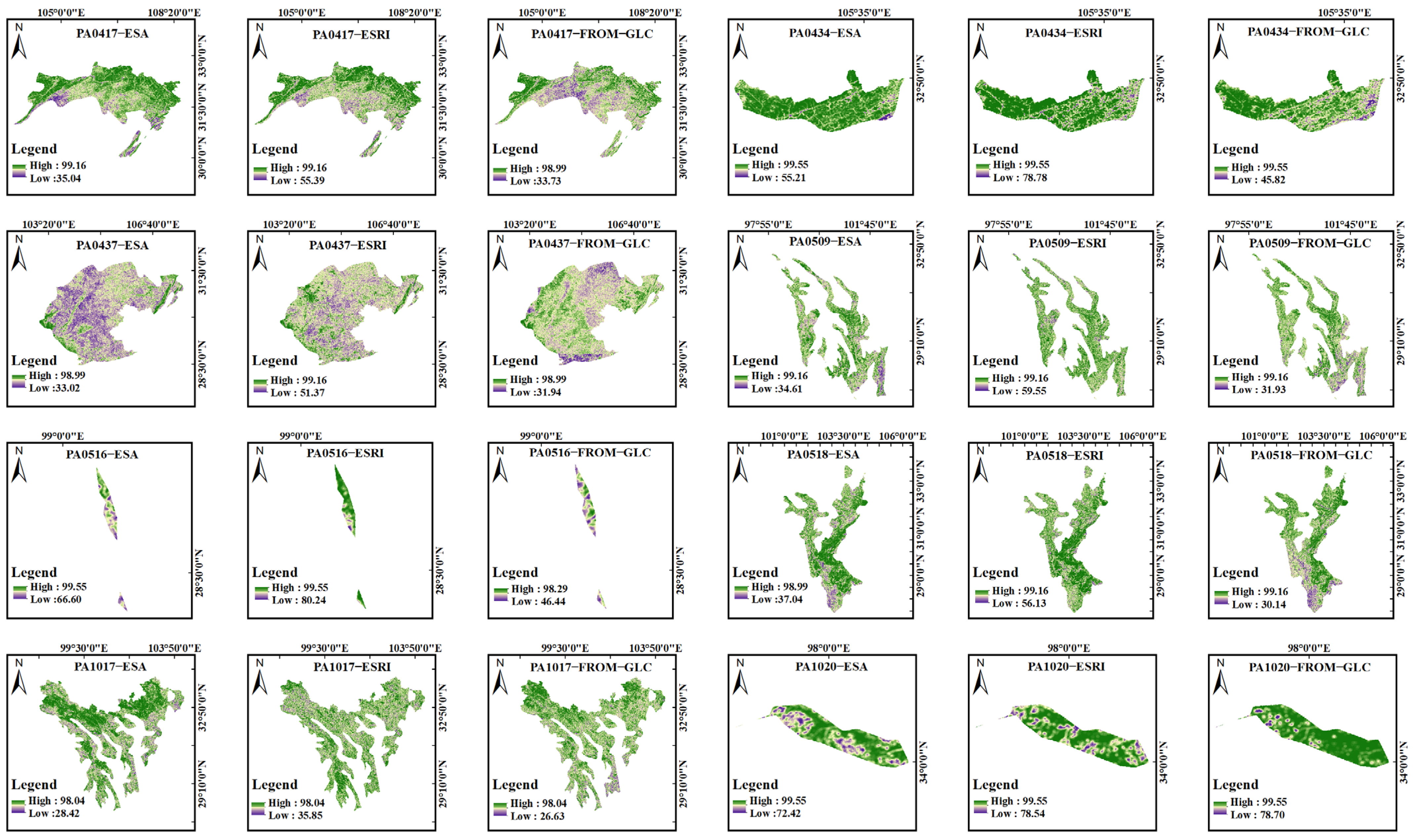
The landscape pattern of AI indices for the three data under different ecoregions is shown in Figure 10. The results indicate that there is some variation in the landscape pattern of AI indices between the three data, which indicated that there were differences in the connectivity between surface landscape patches displayed by the three data. Under the ecological zoning of PA0102, PA0509, PA0516, and PA0518, there was a more consistent distribution of spatial patterns of AI indices for ESA and FROM-GLC land cover data; that is, the connectivity between surface landscape patches reflected by the two kinds of data was relatively consistent. Under the ecological zoning of PA0417 and PA1020, ESA and ESRI land cover data have a relatively consistent distribution of AI index spatial patterns; that is, the connectivity between surface landscape patches reflected by the two data was relatively consistent. Under the ecological zoning of PA0101, PA0434, PA0437, and PA1017, there was a low spatial pattern distribution of AI indices for the three data; that is, the three data showed a large difference in connectivity between surface patches of the landscape.

4.3. Absolute Accuracy Evaluation Based on the Three Independent Validation Samples

The results in

Table 4. Precision evaluation based on Geo-Wiki samples.

Geo-Wiki
		1	2	3	4	5	6	7	8	9	OA (%)	Kappa
FROM-GLC	PA (%)	53.61	48.64	28.89	16.67	0.00	62.50	8.33	37.14	0.00	41.99	0.24
	UA (%)	33.99	73.36	55.32	1.43	0.00	41.67	15.39	13.13	0.00
ESA	PA (%)	67.71	40.28	25.71	25.00	No data	55.56	33.33	20.00	No data	37.86	0.19
	UA (%)	17.39	81.56	57.45	4.29	0.00	41.67	15.39	5.05	0.00
ESRI	PA (%)	64.29	64.11	27.66	14.08	No data	38.46	10.89	41.67	100	39.37	0.25
	UA (%)	23.53	75.41	13.83	41.43	0.00	41.67	84.62	5.05	8.00

Note: 1: Cropland; 2: Forest; 3: Grassland; 4: Shrubland; 5: Wetland; 6: Water; 7: Built-up; 8: Bareland; 9: Snow/Ice.

indicate that the OA and Kappa of FROM-GLC data were the highest, at 41.99% and 0.24, respectively, while the OA and Kappa of ESA data were the lowest, at 37.86% and 0.19, respectively. For each surface cover type precision, the PA and UA of wetland cover types were the lowest, and the three data show serious misclassification and omission errors. The UA of the forest type in FROM-GLC data was higher, at73.36%, indicating that the misclassification error of the forest type was lower. In FROM-GLC data, the PA of the water type was higher, at 62.50%, indicating a lower omission error for water types. The PA of the cropland type in ESA data was higher, at 67.71%, indicating that the omission error of the cropland type was lower. In ESRI data, the UA of the forest and construction types was higher, at 75.41% and 84.62%, respectively, indicating that the misclassification error of the forest and construction types was low.

The experimental results in

Table 5. Precision evaluation based on GLCVSS samples.

GLCVSS
		1	2	3	4	5	6	7	8	9	OA (%)	Kappa
FROM-GLC	PA (%)	53.85	62.75	4.00	No data	No data	0.00	0.00	9.09	No data	38.68	0.18
	UA (%)	35.00	78.05	11.11	0.00	No data	No data	No data	4.55	0.00
ESA	PA (%)	57.14	66.67	18.75	0.00	No data	0.00	0.00	16.67	No data	40.57	0.23
	UA (%)	20.00	78.05	66.67	0.00	No data	No data	No data	4.55	0.00
ESRI	PA (%)	75.00	71.74	0.00	12.12	No data	0.00	0.00	50.00	50.00	42.45	0.27
	UA (%)	30.00	80.49	0.00	66.67	No data	No data	No data	4.55	12.50

Note: 1: Cropland; 2: Forest; 3: Grassland; 4: Shrubland; 5: Wetland; 6: Water; 7: Built-up; 8: Bareland; 9: Snow/Ice.

showed that the OA and Kappa of ESRI data were the highest, at 42.45% and 0.27, respectively, while the OA and Kappa of FROM-GLC data were the lowest, at 38.68% and 0.18, respectively. For each surface cover type precision, the PA and UA of the wetland, water, and construction were low, and the three land cover data showed serious misclassification and omission phenomena. The UA of the forest type in FROM-GLC data was higher, at 78.05%, indicating that the misclassification error of the forest type was lower. In ESA data, the PA and UA of the forest land type were higher, at 66.67% and 78.05%, respectively, indicating that the error of misclassification and omission of the forest type were lower. In ESRI data, the PA of the cropland type was higher, at 75.00%, indicating that the omission error of the cropland type was lower. The UA of the forest type in ESRI data was higher, at 80.49%, indicating that the misclassification error of the forest type was lower.

Experimental results in

Table 6. Evaluation of accuracy based on visual interpretation of samples.

Visual Interpretation
		1	2	3	4	5	6	7	8	9	OA (%)	Kappa
FROM-GLC	PA (%)	86.28	74.57	17.97	0.00	0.00	97.65	82.83	12.07	100	58.40	0.51
	UA (%)	70.40	70.49	82.81	0.00	0.00	61.94	67.21	19.44	25.93
ESA	PA (%)	88.79	73.25	20.37	0.00	91.67	100	93.33	9.33	100	59.87	0.53
	UA (%)	68.59	62.84	85.94	0.00	12.09	76.87	68.85	19.44	18.52
ESRI	PA (%)	92.81	86.26	35.71	3.01	88.89	97.25	61.11	33.33	88.89	55.99	0.50
	UA (%)	51.26	61.75	31.25	44.44	8.79	79.10	99.18	19.44	29.63

Note: 1: Cropland; 2: Forest; 3: Grassland; 4: Shrubland; 5: Wetland; 6: Water; 7: Built-up; 8: Bareland; 9: Snow/Ice.

show that the OA and Kappa of ESA data were the highest, at 59.87% and 0.53, respectively, while the OA and Kappa of ESRI data were the lowest, at 55.99% and 0.50, respectively. The shrubland precision of PA and UA were low, and the three land cover data showed serious misclassification and omission phenomenon. In FROM-GLC data, the PA of the water type was high, at 97.65%, indicating that the omission error of the water type was low. In FROM-GLC data, the UA of the grassland type was higher, at 82.81%, indicating that the misclassification error of the grassland type was lower. In ESA data, the PA of the construction type was higher, at 93.33%, indicating that the omission error of the construction type was low. The UA of the grassland type in ESA data was higher, at 85.94%, indicating that the misclassification error of the grassland type was lower. The ESRI data had a high PA of 97.25% for the water surface type, indicating a low omission error for water. In ESRI data, the UA of the construction type was high, at 99.18%, indicating that the misclassification error of the construction type was low.

5. Discussion

5.1. Analysis of the Impact of Land Cover Landscape Patterns on Research under Ecological Zoning

The land has the characteristics of an ecological environment, such as soil, hydrology, climate, vegetation, and topography. It is a complex of nature and social economy, an important production factor, and a key resource for human survival and development [46,47]. According to Figure 2 of this paper, the land cover types of Sichuan Province are mainly grassland, forest, and cropland, and other types are supplemented. Vegetation types such as grassland, forest, and cropland are very important to the ecological environment and the ecosystem’s service value. The spatial distribution of landscape patterns for grassland, forest, and farmland types in the FROM-GLC, ESA, and ESRI data is shown in Figure 11. It can be found that there are differences in landscape patterns of grassland, forest, and cropland in the three data. For example, the coverage area of the grassland type in ESRI data is small, mainly because the grassland type is determined as the shrubland type in remote sensing recognition of this data. Therefore, the mapping accuracy of vegetation types will significantly influence the results of studies related to ecological zoning (such as the impact of ecosystem service value studies) and even lead to wrong conclusions. In addition, vegetation, as the mainstay of land ecosystems, plays an irreplaceable role in recycling global material and energy, and plays a clear role in reducing atmospheric greenhouse gas concentrations and regulating the global carbon balance [48]. Therefore, the production precision of FROM-GLC, ESA, and ESRI data makes further efforts to improve, and thus to supply, a reference for ecological environment monitoring, land ecological security assessment, and the influence of surface change on vegetation carbon stocks in various ecological zones.

5.2. Discussion of Difference Factors of Multi-Source Remote Sensing Land Cover Data

The landscape patterns of the three data differ to some extent, which is due to the influence of the classification methods, classification systems, and surface complexity used in the generation of the surface cover data [49].

Classification systems are crucial in land cover mapping. The classification system established by land cover producers when producing global-scale land cover data is based primarily on global-scale land information characteristics [50]. This study found that one of the reasons for the large differences in landscape patterns between the three data is the different extraction of some vegetation, such as the type of shrub by the three data, which is inextricably linked to the influence of semantic similarity between the different vegetation types. Therefore, to enhance the precision of future surface cover data acquisition, it is necessary to carefully take into account the clear definition of some vegetation types in the classification system, such as the determination of vegetation cover and tree height element values.

Different classification methods were used to produce FROM-GLC, ESA, and ESRI data. In the production of FROM-GLC data, it is assumed that the training samples of 2015 will be used for the classification of this data under the condition that the land surface type change from 2015 to 2017 is less than 5% [31]. However, this assumption may lead to errors in the mapping accuracy of some seasonal features. When producing ESA land cover data, the L2A product’s scene classification layer was used to eliminate the effect of clouds and shadows on mapping accuracy in the Sentinel-2 data. A 10-day median composite is then calculated from the wavelength time series of data to take away other noise. However, this method of pre-processing ESA data may affect the physical information of the cropland type and thus the precision of the cropland type. Additionally, topographic data were introduced in the cartographic mapping of the three surface cover data. However, there are other data (e.g., vegetation health measurement data) [51] that can reflect the characteristics of seasonal ground features and can be considered in the subsequent mapping to assist in the identification of vegetation (such as grassland), in order to increase the mapping precision of these easily confused vegetation categories.

Furthermore, the number and quality of the validation points obtained for this study covering the region of study also affected the experimental results of this paper. The Geo-wiki and GLCVSS validation samples cover a small number of areas of study compared to the GLCVSS validation samples. Additionally, the accuracy of these two third-party validation samples was not considered in the absolute accuracy evaluation.

In general, the rules for the development of datasets (e.g., classification systems and classification methods) established by different production organizations are a major factor in the variation between products, and this variation leads to significant challenges in the rigorous comparison of maps with each other and the synergistic use of different maps.

5.3. Advantages and Disadvantages of Remote Sensing Technology in Land Cover Data Production

Remote sensing technology has the characteristics of a large coverage area and has free and timely access to data, and has now been used in many fields, such as remote sensing mapping. The development of land cover mapping technology largely depends on the development of remote sensing technology [52,53,54,55]. Google Earth Engine (GEE) is an online data processing platform for planar geospatial analysis, with the enormous computing power of Google’s servers [56]. The three kinds of land cover data analyzed in this paper are all based on the GEE cloud computing platform, and remote sensing mapping of land cover is carried out by using Sentinel series satellites with high spatial resolution. This suggests that the computing power provided by cloud computing can well support producing large surface area cover data using high-resolution satellite remote sensing images. Currently, there is a growing trend of research toward surface cover data production using remote sensing and cloud computing services [57,58,59].

With the advent of the Sentinel series of satellites with higher spatial resolutions, the appearance of data processing tools represented by the GEE and the appearance of more advanced machine learning algorithms, the problems related to remote sensing mapping, such as the use of single-phase images or optical data, will be solved. This has created the conditions for a new generation of land cover mapping characterized by higher resolution and accuracy, as well as less human and material costs.

However, there are certain limitations of surface cover data collection, mainly in the following aspects. (1) A common problem with the current generation of global and regional land cover data is the accuracy of land cover data is low in areas with complex surface landscapes. This is mainly due to the complexity of the surface types in these areas, which are difficult to identify accurately with remote sensing techniques. (2) Some vegetation (such as forests) showed serious confusion owing to the resemble spectral characteristics of ground features. (3) When making global surface cover data, features with smaller patches (such as construction, cropland, etc.,) face great challenges due to their large scale. (4) At present, large area ground cover mapping also mainly adopts a supervised classification strategy based on the training sample, the feasibility, efficiency, and precision of mapping which has certain advantages, but the training sample collection is often an extremely time-consuming, especially for large regional or global scale surface cover mapping samples, which collected a huge workload. On the other hand, the category scheme depends directly on the a priori knowledge of the sample collector.

6. Conclusions

Based on three 10 m worldwide land cover data obtained from geodata, the consistency of the three data under various ecological zones was evaluated using the spatial overlay method, a landscape index for the quantitative evaluation of landscape ecological landscape patterns, and a confusion matrix for three interdependent validation points. The results showed that (1) the spatial consistency of FROM-GLC, ESA, and ESRI data was high in the PA0518 and PA1017 ecological zones, and the area of complete consistency was 44,420.9 km² and 53,368.9 km², respectively. These areas were mainly forest types. The consistency of spatial pattern distribution of these data was low under the PA0509 and PA0437 ecological divisions, which were mainly dispersed in the mountainous areas in the south of Sichuan Province and the Sichuan basin in the east. (2) From the perspective of landscape ecological evaluation, a certain degree of variation in the landscape pattern of the PD, LSI and AI indices of the three data was found under various ecological zones, indicating a low level of landscape fragmentation, landscape morphological complexity, and connectivity between patches. Therefore, it is necessary to be cautious when carrying out studies such as ecological environment monitoring and land ecological security assessment under ecological zoning based on these data. (3) The evaluation results of independent verification points show that the exactitude of the FROM-GLC, ESA, and ESRI data in the study area was low, with an OA of less than 60%. Hence, the future production quality of high-resolution land cover data in the area needs to be further improved.

Although the multiple sets of publicly available high-resolution global land surface data provide precious basic data for many in academic research, these data differ greatly in the landscape patterns of some vegetation types. Therefore, future mapping should be further aimed at improving the accuracy of these key types, or adopt data fusion methods to integrate land cover products from different data sources into high-precision new land cover products.

References

1. Turner, B.; Skole, D.L.; Sanderson, S.; Fischer, G.; Fresco, L.; Leemans, R. Land-use and land-cover change. Science/Research plan. Glob. Change Rep. 1995, 43, 669–679. [Google Scholar]
2. Erb, K.H.; Luyssaert, S.; Meyfroidt, P.; Pongratz, J.; Don, A.; Kloster, S.; Kuemmerle, T.; Fetzel, T.; Fuchs, R.; Herold, M. Land management: Data availability and process understanding for global change studies. Glob. Change Biol. 2017, 23, 512–533. [Google Scholar] [CrossRef] [PubMed] [Green Version]
3. Franklin, J.; Serra-Diaz, J.M.; Syphard, A.D.; Regan, H.M. Big data for forecasting the impacts of global change on plant communities. Glob. Ecol. Biogeogr. 2017, 26, 6–17. [Google Scholar] [CrossRef]
4. Holmberg, M.; Aalto, T.; Akujärvi, A.; Arslan, A.N.; Bergström, I.; Böttcher, K.; Lahtinen, I.; Mäkelä, A.; Markkanen, T.; Minunno, F. Ecosystem services related to carbon cycling–modeling present and future impacts in boreal forests. Front. Plant Sci. 2019, 10, 343. [Google Scholar] [CrossRef] [PubMed]
5. Tolessa, T.; Senbeta, F.; Kidane, M. The impact of land use/land cover change on ecosystem services in the central highlands of Ethiopia. Ecosyst. Serv. 2017, 23, 47–54. [Google Scholar] [CrossRef]
6. Turner, B.L.; Lambin, E.F.; Reenberg, A. The emergence of land change science for global environmental change and sustainability. Proc. Natl. Acad. Sci. USA 2007, 104, 20666–20671. [Google Scholar] [CrossRef] [PubMed] [Green Version]
7. Defourny, P.; Schouten, L.; Bartalev, S.; Bontemps, S.; Cacetta, P.; De Wit, A.; Di Bella, C.; Gérard, B.; Giri, C.; Gond, V. Accuracy assessment of a 300 m global land cover map: The GlobCover experience. New Libr. World 2009, 112, 236–247. [Google Scholar]
8. Loveland, T.R.; Reed, B.C.; Brown, J.F.; Ohlen, D.O.; Zhu, Z.; Yang, L.; Merchant, J.W. Development of a global land cover characteristics database and IGBP DISCover from 1 km AVHRR data. Int. J. Remote Sens. 2000, 21, 1303–1330. [Google Scholar] [CrossRef]
9. Bartholome, E.; Belward, A.S. GLC2000: A new approach to global land cover mapping from Earth observation data. Int. J. Remote Sens. 2005, 26, 1959–1977. [Google Scholar] [CrossRef]
10. Chen, J.; Chen, J.; Liao, A.; Cao, X.; Chen, L.; Chen, X.; He, C.; Han, G.; Peng, S.; Lu, M. Global land cover mapping at 30 m resolution: A POK-based operational approach. ISPRS J. Photogramm. Remote Sens. 2015, 103, 7–27. [Google Scholar] [CrossRef] [Green Version]
11. Bonan, G.B.; Oleson, K.W.; Vertenstein, M.; Levis, S.; Zeng, X.; Dai, Y.; Dickinson, R.E.; Yang, Z.-L. The land surface climatology of the Community Land Model coupled to the NCAR Community Climate Model. J. Clim. 2002, 15, 3123–3149. [Google Scholar] [CrossRef]
12. Feddema, J.J.; Oleson, K.W.; Bonan, G.B.; Mearns, L.O.; Buja, L.E.; Meehl, G.A.; Washington, W.M. The importance of land-cover change in simulating future climates. Science 2005, 310, 1674–1678. [Google Scholar] [CrossRef] [PubMed]
13. Samie, A.; Abbas, A.; Azeem, M.M.; Hamid, S.; Iqbal, M.A.; Hasan, S.S.; Deng, X. Examining the impacts of future land use/land cover changes on climate in Punjab province, Pakistan: Implications for environmental sustainability and economic growth. Environ. Sci. Pollut. Res. 2020, 27, 25415–25433. [Google Scholar] [CrossRef] [PubMed]
14. Tharammal, T.; Bala, G.; Narayanappa, D.; Nemani, R. Potential roles of CO2 fertilization, nitrogen deposition, climate change, and land use and land cover change on the global terrestrial carbon uptake in the twenty-first century. Clim. Dyn. 2019, 52, 4393–4406. [Google Scholar] [CrossRef]
15. Pérez-Hoyos, A.; García-Haro, F.J.; San-Miguel-Ayanz, J. A methodology to generate a synergetic land-cover map by fusion of different land-cover products. Int. J. Appl. Earth Obs. Geoinf. 2012, 19, 72–87. [Google Scholar] [CrossRef]
16. Tsendbazar, N.; De Bruin, S.; Herold, M. Assessing global land cover reference datasets for different user communities. ISPRS J. Photogramm. Remote Sens. 2015, 103, 93–114. [Google Scholar] [CrossRef]
17. Pflugmacher, D.; Krankina, O.N.; Cohen, W.B.; Friedl, M.A.; Sulla-Menashe, D.; Kennedy, R.E.; Nelson, P.; Loboda, T.V.; Kuemmerle, T.; Dyukarev, E.; et al. Comparison and assessment of coarse resolution land cover maps for Northern Eurasia. Remote Sens. Environ. 2011, 115, 3539–3553. [Google Scholar] [CrossRef]
18. Potapov, P.; Tyukavina, A.; Turubanova, S.; Talero, Y.; Hernandez-Serna, A.; Hansen, M.; Saah, D.; Tenneson, K.; Poortinga, A.; Aekakkararungroj, A. Annual continuous fields of woody vegetation structure in the Lower Mekong region from 2000-2017 Landsat time-series. Remote Sens. Environ. 2019, 232, 111278. [Google Scholar] [CrossRef]
19. Zhang, X.; Liu, L.; Chen, X.; Xie, S.; Gao, Y. Fine land-cover mapping in China using Landsat datacube and an operational SPECLib-based approach. Remote Sens. 2019, 11, 1056. [Google Scholar] [CrossRef] [Green Version]
20. Kang, J.; Yang, X.; Wang, Z.; Cheng, H.; Wang, J.; Tang, H.; Li, Y.; Bian, Z.; Bai, Z. Comparison of Three Ten Meter Land Cover Products in a Drought Region: A Case Study in Northwestern China. Land 2022, 11, 427. [Google Scholar] [CrossRef]
21. Wang, J.; Yang, X.; Wang, Z.; Cheng, H.; Kang, J.; Tang, H.; Li, Y.; Bian, Z.; Bai, Z. Consistency Analysis and Accuracy Assessment of Three Global Ten-Meter Land Cover Products in Rocky Desertification Region—A Case Study of Southwest China. ISPRS Int. J. Geo-Inf. 2022, 11, 202. [Google Scholar] [CrossRef]
22. Giri, C.; Zhu, Z.; Reed, B. A comparative analysis of the Global Land Cover 2000 and MODIS land cover data sets. Remote Sens. Environ. 2005, 94, 123–132. [Google Scholar] [CrossRef]
23. Yang, Y.; Xiao, P.; Feng, X.; Li, H. Accuracy assessment of seven global land cover datasets over China. ISPRS J. Photogramm. Remote Sens. 2017, 125, 156–173. [Google Scholar] [CrossRef]
24. Chen, X.; Lin, Y.; Zhang, M.; Yu, L.; Li, H.; Bai, Y. Assessment of the cropland classifications in four global land cover datasets: A case study of Shaanxi Province, China. J. Integr. Agric. 2017, 16, 298–311. [Google Scholar] [CrossRef] [Green Version]
25. Kang, J.; Sui, L.; Yang, X.; Wang, Z.; Huang, C.; Wang, J. Spatial Pattern Consistency among DifferentRemote-Sensing Land Cover Datasets: A Case Studyin Northern Laos. ISPRS Int. J. Geo-Inf. 2019, 8, 201. [Google Scholar] [CrossRef] [Green Version]
26. Liang, L.; Liu, Q.; Liu, G.; Li, H.; Huang, C. Accuracy evaluation and consistency analysis of four global land cover products in the Arctic region. Remote Sens. 2019, 11, 1396. [Google Scholar] [CrossRef] [Green Version]
27. Hua, T.; Zhao, W.; Liu, Y.; Wang, S.; Yang, S. Spatial consistency assessments for global land-cover datasets: A comparison among GLC2000, CCI LC, MCD12, GLOBCOVER and GLCNMO. Remote Sens. 2018, 10, 1846. [Google Scholar] [CrossRef] [Green Version]
28. Liang, D.; Zuo, Y.; Huang, L.; Zhao, J.; Teng, L.; Yang, F. Evaluation of the consistency of MODIS Land Cover Product (MCD12Q1) based on Chinese 30 m GlobeLand30 datasets: A case study in Anhui Province, China. ISPRS Int. J. Geo-Inf. 2015, 4, 2519–2541. [Google Scholar] [CrossRef] [Green Version]
29. Bai, Y.; Feng, M.; Jiang, H.; Wang, J.; Zhu, Y.; Liu, Y. Assessing consistency of five global land cover data sets in China. Remote Sens. 2014, 6, 8739–8759. [Google Scholar] [CrossRef] [Green Version]
30. Liu, L.; Zhang, X.; Gao, Y.; Chen, X.; Shuai, X.; Mi, J. Finer-resolution mapping of global land cover: Recent developments, consistency analysis, and prospects. J. Remote Sens. 2021, 2021, 5289697. [Google Scholar] [CrossRef]
31. Chen, B.; Xu, B.; Zhu, Z.; Yuan, C.; Suen, H.P.; Guo, J.; Xu, N.; Li, W.; Zhao, Y.; Yang, J. Stable classification with limited sample: Transferring a 30-m resolution sample set collected in 2015 to mapping 10-m resolution global land cover in 2017. Sci. Bull 2019, 64, 370–373. [Google Scholar]
32. Karra, K.; Kontgis, C.; Statman-Weil, Z.; Mazzariello, J.C.; Mathis, M.; Brumby, S.P. Global land use/land cover with Sentinel 2 and deep learning. In Proceedings of the 2021 IEEE International Geoscience and Remote Sensing Symposium IGARSS, Brussels, Belgium, 11–16 July 2021; pp. 4704–4707. [Google Scholar]
33. Zhang, J.; Qian, Z.; Wanggu, X.; Zhang, H.; Wang, Z. Ecosystem pattern variation from 2000 to 2010 in national nature reserves of China. Acta Ecol. Sin 2017, 37, 8067–8076. [Google Scholar]
34. Frost, G.V.; Epstein, H.E.; Walker, D.A.; Matyshak, G.; Ermokhina, K. Seasonal and long-term changes to active-layer temperatures after tall shrubland expansion and succession in Arctic tundra. Ecosystems 2018, 21, 507–520. [Google Scholar] [CrossRef]
35. Sturm, M.; Schimel, J.; Michaelson, G.; Welker, J.M.; Oberbauer, S.F.; Liston, G.E.; Fahnestock, J.; Romanovsky, V.E. Winter biological processes could help convert arctic tundra to shrubland. Bioscience 2005, 55, 17–26. [Google Scholar] [CrossRef]
36. Olson, D.M.; Dinerstein, E.; Wikramanayake, E.D.; Burgess, N.D.; Powell, G.V.; Underwood, E.C.; D’amico, J.A.; Itoua, I.; Strand, H.E.; Morrison, J.C. Terrestrial Ecoregions of the World: A New Map of Life on EarthA new global map of terrestrial ecoregions provides an innovative tool for conserving biodiversity. BioScience 2001, 51, 933–938. [Google Scholar] [CrossRef]
37. Sun, B.; Zhou, Q. Expressing the spatio-temporal pattern of farmland change in arid lands using landscape metrics. J. Arid Environ. 2016, 124, 118–127. [Google Scholar] [CrossRef]
38. Wang, J.; Wang, Z.; Cheng, H.; Kang, J.; Liu, X. Land Cover Changing Pattern in Pre-and Post-Earthquake Affected Area from Remote Sensing Data: A Case of Lushan County, Sichuan Province. Land 2022, 11, 1205. [Google Scholar] [CrossRef]
39. Canters, F. Evaluating the uncertainty of area estimates derived from fuuy land-cover classification. Photogramm. Eng. Remote Sens. 1997, 63, 403–414. [Google Scholar]
40. Clark, M.L.; Aide, T.M.; Grau, H.R.; Riner, G. A scalable approach to mapping annual land cover at 250 m using MODIS time series data: A case study in the Dry Chaco ecoregion of South America. Remote Sens. Environ. 2010, 114, 2816–2832. [Google Scholar] [CrossRef]
41. Kang, J.; Wang, Z.; Cheng, H.; Wang, J.; Liu, X. Remote Sensing Land Use Evolution in Earthquake-Stricken Regions of Wenchuan County, China. Sustainability 2022, 14, 9721. [Google Scholar] [CrossRef]
42. Fung, T.; Ledrew, E.F. The determination of optimal threshold levels for change detection using various accuracy indices. Photogramm. Eng. Remote Sens. 1988, 54, 1449–1454. [Google Scholar]
43. Yang, J.; Huang, X. The 30 m annual land cover dataset and its dynamics in China from 1990 to 2019. Earth Syst. Sci. Data 2021, 13, 3907–3925. [Google Scholar] [CrossRef]
44. Fritz, S.; See, L.; Perger, C.; Mccallum, I.; Schill, C.; Schepaschenko, D.; Duerauer, M.; Karner, M.; Dresel, C.; Laso-Bayas, J.C. A global dataset of crowdsourced land cover and land use reference data. Sci. Data 2017, 4, 170075. [Google Scholar] [CrossRef] [Green Version]
45. Zhao, Y.; Gong, P.; Yu, L.; Hu, L.; Li, X.; Li, C.; Zhang, H.; Zheng, Y.; Wang, J.; Zhao, Y.; et al. Towards a common validation sample set for global land-cover mapping. Int. J. Remote Sens. 2014, 35, 4795–4814. [Google Scholar] [CrossRef]
46. Verburg, P.H.; Steeg, J.; Veldkamp, A.; Willemen, L. From land cover change to land function dynamics: A major challenge to improve land characterization. J. Environ. Manag. 2009, 90, 1327–1335. [Google Scholar] [CrossRef]
47. Correia Filho, W.L.F.; de Oliveira-Júnior, J.F.; dos Santos, C.T.B.; Batista, B.A.; de Barros Santiago, D.; da Silva Junior, C.A.; Teodoro, P.E.; da Costa, C.E.S.; da Silva, E.B.; Freire, F.M. The influence of urban expansion in the socio-economic, demographic, and environmental indicators in the City of Arapiraca-Alagoas, Brazil. Remote Sens. Appl. Soc. Environ. 2022, 25, 100662. [Google Scholar] [CrossRef]
48. Mathias, J.M.; Trugman, A.T. Climate change impacts plant carbon balance, increasing mean future carbon use efficiency but decreasing total forest extent at dry range edges. Ecol. Lett. 2022, 25, 498–508. [Google Scholar] [CrossRef]
49. Gao, Y.; Liu, L.; Zhang, X.; Chen, X.; Mi, J.; Xie, S. Consistency analysis and accuracy assessment of three global 30-m land-cover products over the European Union using the LUCAS dataset. Remote Sens. 2020, 12, 3479. [Google Scholar] [CrossRef]
50. Kang, J.; Wang, Z.; Sui, L.; Yang, X.; Ma, Y.; Wang, J. Consistency analysis of remote sensing land cover products in the tropical rainforest climate region: A case study of Indonesia. Remote Sens. 2020, 12, 1410. [Google Scholar] [CrossRef]
51. Phan, T.N.; Kuch, V.; Lehnert, L.W. Land Cover Classification using Google Earth Engine and Random Forest Classifier—The Role of Image Composition. Remote Sens. 2020, 12, 2411. [Google Scholar] [CrossRef]
52. Mahdianpari, M.; Salehi, B.; Rezaee, M.; Mohammadimanesh, F.; Zhang, Y. Very deep convolutional neural networks for complex land cover mapping using multispectral remote sensing imagery. Remote Sens. 2018, 10, 1119. [Google Scholar] [CrossRef] [Green Version]
53. Huang, B.; Zhao, B.; Song, Y. Urban land-use mapping using a deep convolutional neural network with high spatial resolution multispectral remote sensing imagery. Remote Sens. Environ. 2018, 214, 73–86. [Google Scholar] [CrossRef]
54. Li, X.; Sun, C.; Meng, H.; Ma, X.; Huang, G.; Xu, X. A Novel Efficient Method for Land Cover Classification in Fragmented Agricultural Landscapes Using Sentinel Satellite Imagery. Remote Sens. 2022, 14, 2045. [Google Scholar] [CrossRef]
55. Sarif, M.; Gupta, R.D. Spatiotemporal mapping of Land Use/Land Cover dynamics using Remote Sensing and GIS approach: A case study of Prayagraj City, India (1988–2018). Environ. Dev. Sustain. 2022, 24, 888–920. [Google Scholar] [CrossRef]
56. Gorelick, N.; Hancher, M.; Dixon, M.; Ilyushchenko, S.; Thau, D.; Moore, R. Google Earth Engine: Planetary-scale geospatial analysis for everyone. Remote Sens. Environ. 2017, 202, 18–27. [Google Scholar] [CrossRef]
57. de Sousa, C.; Fatoyinbo, L.; Neigh, C.; Boucka, F.; Angoue, V.; Larsen, T. Cloud-computing and machine learning in support of country-level land cover and ecosystem extent mapping in Liberia and Gabon. PLoS ONE 2020, 15, e0227438. [Google Scholar] [CrossRef] [PubMed]
58. Midekisa, A.; Holl, F.; Savory, D.J.; Andrade-Pacheco, R.; Gething, P.W.; Bennett, A.; Sturrock, H.J. Mapping land cover change over continental Africa using Landsat and Google Earth Engine cloud computing. PLoS ONE 2017, 12, e0184926. [Google Scholar] [CrossRef]
59. Kang, J.; Yang, X.; Wang, Z.; Huang, C.; Wang, J. Collaborative Extraction of Paddy Planting Areas with Multi-Source Information Based on Google Earth Engine: A Case Study of Cambodia. Remote Sens. 2022, 14, 1823. [Google Scholar] [CrossRef]
Figure 1. Spatial location distribution of the study area.
Sustainability 14 16673 g001
Figure 2. Spatial distributions of the three data: (a) FROM-GLC, (b) ESA, and (c) ESRI.
Sustainability 14 16673 g002
Figure 3. The spatial distribution of terrestrial ecological zones.
Sustainability 14 16673 g003
Figure 4. Schematic diagram of spatial pattern consistency. Legend: Type: 1: Cropland; 0: Other; Overlay results: 0: background; 1: Completely inconsistent; 2: Basically consistent; 3: Completely consistent.
Sustainability 14 16673 g004
Figure 5. The spatial distribution of samples: (a) Geo-Wiki, (b) GLCVSS, and (c) Visual interpretation.
Sustainability 14 16673 g005
Figure 6. Spatial consistency distribution map in TEOW.
Sustainability 14 16673 g006
Figure 7. Spatial consistency area statistics in TEOW.
Sustainability 14 16673 g007
Figure 8. PD comparison of the three land cover data in different TEOW.
Sustainability 14 16673 g008
Figure 9. LSI comparison of the three land cover data in different TEOW.
Sustainability 14 16673 g009
Figure 10. AI comparison of the three land cover data in different TEOW.
Sustainability 14 16673 g010aSustainability 14 16673 g010b
Figure 11. Landscape pattern distribution of grassland, forest, and cropland of the three land cover data.
Sustainability 14 16673 g011aSustainability 14 16673 g011b