Optimization Method of Combined Multi-Mode Bus Scheduling under Unbalanced Conditions

Abstract

In view of the spatial and temporal imbalance of residents’ travel demands and challenges of optimal bus capacity allocation, in this paper the grand station express bus scheduling mode is introduced in the direction of heavy passenger flow during peak hours. Coordinated scheduling combining whole-journey and grand station express buses is adopted, and the station correlation calculation model is used to determine the optimal stops of the grand station express bus. Thus, a two-way bus scheduling optimization model for peak passenger flow is established with the goal of minimizing the total cost of passenger travel and enterprise operation. Finally, the nonlinear inertia weight dynamic cuckoo search algorithm is selected for the model’s solution, and the established scheduling optimization model is solved by combining basic data such as the study line’s bus Integrated Circuit (IC) card data. The effectiveness of the model is verified through a comparative study and evaluation of the solution.

1. Introduction

At present, due to temporal and spatial imbalances of residents’ travel demands, the disparity between supply and demand of bus services is growing, which seriously affects the service quality and inhibits the effective implementation of strategies based on need priority. In the bus line, traditional single-bus scheduling modes have limited benefits and do not match the travel demand characteristics of contemporary urban bus service users. It is therefore urgent to implement refined and systematic multi-mode bus scheduling schemes. In recent years, the problem of bus operation scheduling optimization has been studied mainly from the aspects of planning and scheduling control.

The preparation of a bus service plan mainly involves establishing a mathematical model to describe the actual bus scheduling problem and using relevant algorithms to find optimal solutions for that model. Based on the cost of passenger travel and vehicle operators, Malacly [1] focused on the cost of passengers’ planned travel time and the cost of vehicles’ late arrival and studied the preparation of bus schedules. Stephan [2] created a schedule containing multiple vehicle types based on the network program to solve the multi-objective problem of minimizing the expected waiting time of passengers and the expected vehicle occupancy levels. The method resulted in a more than 43% reduction of the waiting time of passengers in a practical application. Avishai [3] proposed a method combining uniform headway and load to create a schedule and developed a heuristic algorithm to solve this kind of cost flow network problem with an NP-hard complexity level. James [4] proposed a mixed integer linear programming model to solve the transfer synchronization planning problem of bus timetables. This model simultaneously optimized the bus timetable and passenger travel path selection through a heuristic algorithm, resulting in highly accurate bus timetables. Mizuyo [5] discussed schedule design in low-frequency bus service areas and proposed a mathematical optimization model to generate a modified bus schedule that shortened the transfer waiting time of passengers effectively. Berrebi et al. [6] proposed a real-time waiting mechanism to ensure that high-frequency lines in operation can maintain a stable headway and avoid congestion in buses and found the optimal holding strategy through reverse induction. Gkiotsalitis [7] adopted a periodic optimization method that reacted to the disturbance of bus travel times and passenger demand to model the scheduling time control problem in a rolling section. This model allows traffic planners to adjust the bus schedule in daily operations and has stronger flexibility.

With the urgent demand for improving the service level of bus systems, intelligent and real-time scheduling approaches have emerged and become the current research direction and hotspot. Adamski [8] proposed a real-time online adaptive scheduling control problem for dynamically modeling public transit lines and investigated numerical solutions. Horn [9] described a deployment system for managing demand-responsive passenger vehicle fleets (such as taxis or variable route buses) with the goal of local minimization of travel time. Compared with traditional scheduling methods, this system was more efficient. Dakic et al. [10] developed a flexible bus scheduling system consisting of a fleet of fully automated modular bus units along with conventional buses to meet passenger demands and proposed an optimization model for determining the optimal frequency of service to be dispatched on each bus route. Yang et al. [11] considered the correlation between Bus Rapid Transit vehicle types, passenger waiting times and vehicle energy consumption, and they established a multi-objective Bus Rapid Transit energy-saving scheduling optimization model with the goal of minimizing passenger waiting time and vehicle energy consumption, thereby reducing vehicle energy consumption and passenger waiting times effectively. In order to meet the unbalanced demand of passengers on bus lines and improve the service level of bus lines, Zhang et al. [12] evaluated the degree of imbalance and considered the impact of station-hopping behavior and bus capacity on the remaining passengers. By minimizing the waiting time of passengers, the time in the bus and the running time of vehicles, they determined appropriate stops for the bus fleet serving the entire route. Luo et al. [13] proposed a dynamic bus scheduling optimization model to minimize the total waiting time of passengers, while Huang et al. [14] proposed a dynamic bus scheduling model based on the arrival time of bus vehicles and the prediction of bus passenger flow. Compared with the real-time lag strategy, this method reduces the waiting time of passengers effectively.

In terms of bus scheduling optimization, most researchers still focus on conventional scheduling methods. When unbalanced lines are assumed, the method of adjusting the two-way departure interval is commonly adopted, or a one-way combined scheduling scheme is investigated, and research on two-way multi-mode combined scheduling with unbalanced lines is seldom encountered. To determine the optimal corresponding solutions of the established models, scholars have used many algorithms, but most are genetic algorithms, particle swarm optimization algorithms and other earlier algorithms, and there is little innovation in these approaches.

The bus scheduling optimization model established in this paper can better match the passenger flow distribution of the line, thus reducing the comprehensive cost of passenger travel and bus enterprise operation effectively. This is highly important, as it is of great significance to improve the utilization rate of bus resources, the bus service level and share rate. At the same time, in this study, a new algorithm design is also introduced to solve the bus scheduling problem, which can provide reference for the future research and selection of scheduling model algorithms.

2. Selection of Fast Bus Stops at Large Stations

In order to deeply analyze and mine the relationship between different stops on a bus line, in this paper the association degree between each stop is analyzed based on the station association degree so as to determine the stops of grand station express vehicles in the direction of heavy passenger flow during peak hours. Common types of bus stops are shown in Figure 1.

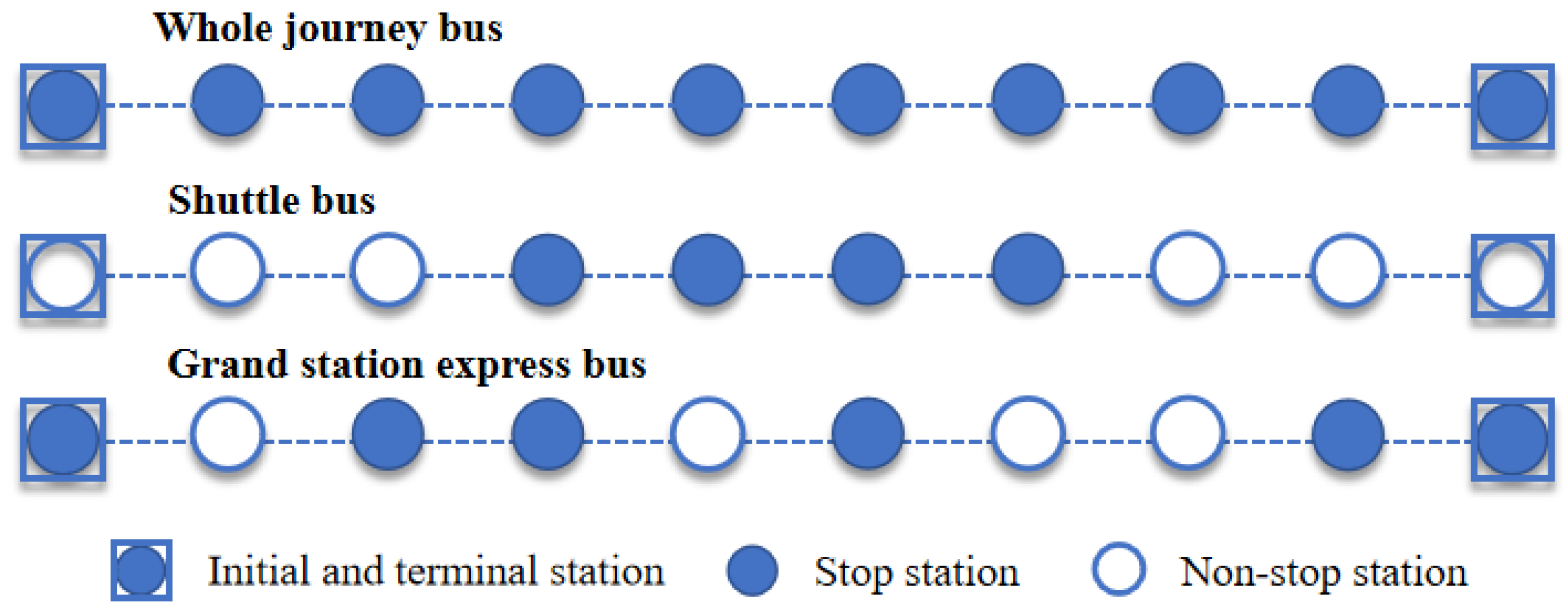
2.1. Type of Bus Scheduling

At present, common scheduling forms pertain to whole-journey buses, shuttle buses and grand station express buses [15]. A schematic diagram of these different scheduling forms is shown in Figure 2. Depending on the passenger flow distribution of the bus lines, a single form, most commonly the whole-journey bus, or a combination of any two or three of these forms will be selected. In view of the increased passenger flows in morning and evening peak hours, the imbalances between the coefficients of direction, boarding and alighting at some stations in the direction of heavy passenger flow are large. As passenger boarding and alighting stations are relatively concentrated in these cases, the grand station express bus scheduling mode can be introduced in the direction of heavy passenger flow, and the coordinated scheduling of whole-journey and grand station express buses can be adopted.

2.2. Calculation Model of Site Relevance

The station correlation degree refers to the correlation degree between two stations in a bus line. Generally, a higher correlation degree between stations A and B reflects a stronger tendency of passengers embarking at station A (B) to disembark at station B (A). In this paper, the station correlation degree is analyzed according to the association rules [16].

Association rules are a widely used in pattern recognition methods. The strength of association can be measured using support and confidence, where support represents the probability of both A and B occurring simultaneously in the rule, while confidence represents the probability of B occurring if A has occurred [17]. The calculation equations of the two rules are as follows:

$$\left\{\begin{array}{c}support(A\to B)=P\left(A\cup B\right)\begin{array}{ccc}& & \end{array}\\ confidence(A\to B)=\frac{support\left(A\cup B\right)}{support\left(A\right)}\end{array}\right.$$

(1)

In this study, the item set support degree is the percentage of passengers embarking at station j and disembarking at station n compared to the total number of passengers on the whole line. The item set confidence degree is the percentage of passengers embarking on at station j and disembarking at station n to the total number of passengers embarking at station j. The calculation equation considering the station passenger flow comprehensively is:

$$\left\{\begin{array}{c}support(j\to n)=\frac{g_{jn}}{{\displaystyle \sum _{j=1}^J{q}_j}}\cdot 100\%\\ confidence(j\to n)=\frac{g_{jn}}{q_j}\cdot 100\%\end{array}\right.$$

(2)

where g_jn is the number of passengers embarking at station j and disembarking at station n (in persons), while q_j is the total number of passengers embarking at station j.

2.3. Optimization of Line Stops

Based on its definition, it can be seen that the support degree has a direct relationship with the collection and distribution volume of passenger flow on the line and should at least reach the average value when selecting large-station express stops in practical problems. Therefore, Equation (3) can be used to determine the selection threshold of the first round of stops:

$$SU=\eta \frac{1}{J-1}\cdot 100\%$$

(3)

where SU is the support screening threshold; $\eta$ is a coefficient, whose value lies in the range 1.0~1.8 depending on the actual situation of the line; and J is the total number of stations along the line.

The degree of support quantifies the distribution of passenger flow at each station on the whole line, while the degree of confidence is suitable for describing the passenger flow between stations. Therefore, after screening out first round of stations, it is necessary to add confidence indicators for the second round of station selection. Based on the confidence calculation results among the sites, the sites with the highest confidence during the first round of selection in the uplink and downlink directions are selected.

3. Bus Scheduling Optimization Model under Unbalanced Conditions

In order to improve the convenience and comfort of bus travel, passengers require reduced waiting and travel times, while bus companies aim to reduce the investment required in vehicles and personnel to reduce operating costs. In order to maximize the comprehensive benefits, it is necessary to find a balance between the interests of the two. Therefore, bus scheduling optimization is a multi-objective optimization problem aiming to minimize passenger travel time and maximize enterprise benefits, with waiting time, onboard time and operating costs being the minimization objectives. In this study, two-way scheduling is analyzed, and the sum of the total costs of two-way passenger travel and two-way operation of the bus enterprise is minimized as the objective function to determine the optimal departure interval of upstream and downstream bus vehicles.

3.1. Model Assumptions and Establishment Steps

To facilitate the study, the following assumptions are made about the actual situation before building the model.

• The arrival time of passengers at each stop during the study period obeys a uniform distribution.
• Passengers embark on the first bus at the bus stop within the travel interval, and they do not wait for a second bus to come along.
• There is no transfer between the whole-journey bus and the grand station express bus.
• All vehicles operating on the same route are of the same type, rated passenger capacity and maximum passenger capacity, and these values are fixed.
• Each line’s operation is independent and not affected by neighboring lines.
• Bus vehicles move in strict accordance with the schedule and are on time.
• The speed of bus vehicles between stations is constant regardless of road operating hours and weather conditions, ignoring traffic jams or other unexpected circumstances encountered, and stations can be reached on time.

Two-Way Bus Scheduling Optimization Model for Peak Passenger Flow model building steps are shown in detail below.

Step 1: Calculate the bus passenger travel cost. Bus passenger travel cost includes passenger waiting cost $C_w$ and passenger travel cost $C_o$. Among them, passenger waiting cost $C_w$ includes passenger waiting cost $C_{wg}$ in the heavy passenger flow direction (HPFD) and passenger waiting cost $C_{wq}$ in the light passenger flow direction (LPFD), and passenger travel cost $C_o$ includes passenger travel cost $C_{oq}$ in the LPFD and passenger travel cost $C_{og}$ in the HPFD.

Step 2: Calculate the bus enterprise operating cost. The bus enterprise operating cost includes the operating cost $C_{qq}$ in the LPFD and the bus enterprise operating cost $C_{qg}$ in the HPFD.

Step 3: Establish the objective function of the two-way bus scheduling optimization model for peak passenger flow.

Step 4: Establish the constraints of the model. The constraints are the maximum and minimum interval between departures and minimum load rate.

3.2. Two-Way Bus Scheduling Optimization Model for Peak Passenger Flow

Aiming at the problems of large passenger flow in peak hours, considering the large disequilibrium coefficient in the direction of heavy passenger flow and large disequilibrium coefficient between passengers on and off at some stations in the direction of heavy passenger flow, and taking the bus passenger travel cost and bus enterprise operating cost as optimization objectives, the two-way bus scheduling optimization model for peak passenger flow was established.

3.2.1. Bus Passenger Travel Costs

In this study, the passenger travel cost associated with bus scheduling is mainly considered as comprising the two components of bus passengers’ waiting cost and passengers’ on-board cost, which are expressed in the following forms.

$$C_c=C_w+C_o$$

(4)

where $C_c$ is the cost of bus passenger travel, $C_w$ is the cost of passengers’ waiting and $C_o$ is the cost associated with the passengers’ travel time.

(1)

Passenger waiting cost $C_w$.

From the model assumptions, within a travel interval $\Delta t_i$, the passenger arrival time at each station obeys a uniform distribution, so the average time passengers need to wait for the ith bus to arrive is:

$$\frac{(t_i-t_{i-1})}{2}=\frac{\Delta t_i}{2}$$

(5)

Therefore, the waiting cost $C_{wq}$ for passengers in the light passenger flow direction (LPFD) is:

$$C_{wq}=\rho \cdot {\displaystyle \sum _{i_{kq}=1}^{I_{kq}}{\displaystyle \sum _{j_q=1}^{J_q-1}{\displaystyle \sum _{n_q=j_q+1}^{J_q}{q}_{j_q,n_q}^{i_{kq}}}\cdot \frac{t_{kq}}{2}}}$$

(6)

where $\rho$ is the bus passenger waiting time cost coefficient, established from the local residents’ working day per capita wage, in RMB/minute;$I_{kq}$ is the total number of departures along the LPFD during the k-th scheduling period; $i_{kq}$ is the $i_{kq}$-th vehicle on the LPFD during the k-th scheduling period, with $0<i_{kq}\le I_{kq}$; $J_q$ is the total number of stops in the LPFD of the bus line; $j_q$ is the $j_q$-th stop in the light passenger direction, where $0<j_q<J_q$; $n_q$ is the $n_q$-th stop on the LPFD, with $1<n_q\le J_q$; $q_{j_q,n_q}^{i_{kq}}$ is the number of passengers who take the vehicle of schedule $i_q$ from station $j_q$ to station $n_q$ in the LPFD during scheduling period k; and $t_{kq}$ is the departure interval of the LPFD during the k-scheduling period, in seconds.

Since a combination of the whole-journey bus and a grand station express bus is used in the heavy passenger flow direction (HPFD), the corresponding waiting cost $C_{wg}$ for passengers is:

$$C_{wg}=\rho \cdot {\displaystyle \sum _{i_{kg}=1}^{I_{kg}}[{\displaystyle \sum _{j_g=1}^{J_g-1}{\displaystyle \sum _{n_g=j_g+1}^{J_g}{q}_{j_g,n_g}^{i_{kg}}\cdot {\theta }_{j_g}^{i_g}\cdot {\theta }_{n_g}^{i_g}\cdot \frac{t_{kg1}+t_{kg2}}{2}+(Z-{\displaystyle \sum _{j_g=1}^{J_g-1}{\displaystyle \sum _{n_g=j_g+1}^{J_g}{q}_{j_g,n_g}^{i_{kg}}\cdot {\theta }_{j_g}^{i_g}\cdot {\theta }_{n_g}^{i_g}}})\cdot \frac{t_{kg1}}{2}}}}]$$

(7)

where $I_{kg}$ is the total number of trips on the HPFD during the k-th scheduling period; $i_{kg}$ is the $i_{kg}$-th vehicle on the HPFD during the k-th scheduling period, with $0<i_{kg}\le I_{kg}$; $J_g$ is the total number of stops on the HPFD of the bus line; $j_g$ is the $j_g$-th station in the HPFD, where $0<j_g\le J_g$; $n_g$ is the $n_g$-th station in the HPFD, with $0<n_g\le J_g$; $q_{j_g,n_g}^{i_{kg}}$ is the number of passengers who take the vehicle of schedule $i_{kg}$ and embark at station $j_g$ and disembark at station $n_g$ during the k-th scheduling period; ${\theta }_{j_g}^{i_g}$ and ${\theta }_{n_g}^{i_g}$ are binary variables, for which when the vehicle of schedule $i_g$ in the HPFD stops at station $j_g$, ${\theta }_{j_g}^{i_g}=1$, and otherwise it is 0, and accordingly for ${\theta }_{n_g}^{i_g}$; $t_{kg1}$ is the departure interval of the whole-journey bus along the HPFD during the k-th scheduling period, in minutes; and $t_{kg1}$ is the departure interval of the express bus along the HPFD during the k-th scheduling period, in minutes.

The total number of passengers of the bus line is defined as Z, as shown in Equation (8).

$$Z={\displaystyle \sum _{j_g=1}^{J_g-1}{\displaystyle \sum _{n_g=j_g+1}^{J_g}{q}_{j_g,n_g}^{i_{kg}}}}$$

(8)

(2)

Passenger travel cost $C_o$.

The passenger on-boarding cost refers to the cost of time consumed by passengers on the bus [18,19]. This cost mainly includes the section travel time and station stopping time. For the convenience of the study, it is assumed that the bus vehicle travels at a constant speed between stops and that the vehicle running time in the model is only related to the stop distance and travel speed. When buses are in stations, they usually need to meet passenger boarding and alighting demands at the same time, so the vehicle station stopping time is the larger of the passenger boarding time and alighting time.

$$T_{ij}^k=\max \left\{{\overline{t}}_{up}{U}_{ij}^k,{\overline{t}}_{down}{D}_{ij}^k\right\}$$

(9)

where, ${\overline{t}}_{up}$ and ${\overline{t}}_{down}$ are the per capita boarding and alighting times of bus passengers, respectively, in s.

The number of passengers boarding the vehicle of schedule i at stop j during the scheduling period k is $U_{ij}^k$, while the number of passengers alighting at stop j is $D_{ij}^k$. Therefore, the cross-sectional passenger flow $P_{i,j\to j+1}^k$ of a bus operating in the interval from station j to station j + 1 is:

$$P_{i,j\to j+1}^k=P_{i,j-1\to j}^k+U_{ij}^k-D_{ij}^k$$

(10)

Therefore, the cost $C_{oq}$ of passenger travel in the LPFD is:

$$C_{oq}={\rho }^{\prime }\cdot {\displaystyle \sum _{i_q=1}^{I_{kq}}{\displaystyle \sum _{j_q=1}^{J_q}[t_{j_q\to j_q+1}^k}}\cdot (P_{i_q,j_q-1\to j_q}^k+U_{i_q{j}_q}^k-D_{i_q{j}_q}^k)+T_{i_q{j}_q}^k\cdot (P_{i_q,j_q-1\to j_q}^k-D_{i_q{j}_q}^k)]$$

(11)

where ${\rho }^{\prime }$ is the cost coefficient of bus passenger travel time, obtained by converting the per capita wage of local residents on working days, in RMB/minute; $t_{j_q\to j_q+1}^k$ is the average running time of bus vehicles from station $j_q$ to station $j_q+1$, in seconds; $U_{i_q{j}_q}^k$ is the number of passengers embarking at station $j_q$ on the vehicle of schedule $i_q$ in the LPFD during the k-th scheduling period; $D_{i_q{j}_q}^k$ is the number of passengers disembarking at station $j_q$ from the vehicle of schedule $i_q$ in the LPFD during the k-th scheduling period;$P_{i_q,j_q-1\to j_q}^k$ is the cross-sectional passenger flow from the vehicle of schedule $i_q$ in the LPFD running in the interval from station $j_q-1$ to station $j_q$ during the k-th scheduling period; and $T_{i_q{j}_q}^k$ is the stopping time of the vehicle of schedule $i_q$ in the LPFD at station $j_q$ during the k-th scheduling period, in seconds.

The cost $C_{og}$ of passenger travel along the HPFD under the coordinated scheduling of whole-journey and grand station express buses is:

$$C_{og}={\rho }^{\prime }\cdot {\displaystyle \sum _{i_g=1}^{I_{kg}}{\displaystyle \sum _{j_g=1}^{J_g}[t_{j_g\to j_g+1}^k}}\cdot (P_{i_g,j_g-1\to j_g}^k+U_{i_g{j}_g}^k-D_{i_g{j}_g}^k)+{\theta }_{j_g}^{i_g}\cdot T_{i_g{j}_g}^k\cdot (P_{i_g,j_g-1\to j_g}^k-D_{i_g{j}_g}^k)]$$

(12)

where $t_{j_g\to j_g+1}^k$ is the average running time of bus vehicles along the HPFD from station $j_g$ to station $j_g+1$, in seconds; $U_{i_g{j}_g}^k$ is the number of passengers embarking at station $j_g$ on the vehicle of schedule $i_g$ in the HPFD during the k-th scheduling period; $D_{i_g{j}_g}^k$ is the number of passengers disembarking at station $j_g$ from the vehicle of schedule $i_g$ in the HPFD during the k-th scheduling period; $P_{i_g,j_g-1\to j_g}^k$ is the cross-sectional passenger flow from the vehicle of schedule $i_g$ in the HPFD running in the interval from station $j_g-1$ to station $j_g$ during the k-th scheduling period; and $T_{i_g{j}_g}^k$ is the stopping time of the vehicle of schedule $i_g$ in the HPFD at station $j_g$ during the k-th scheduling period, in seconds.

3.2.2. Bus Enterprise Operating Costs

The bus enterprise operation cost refers to the cost paid by the bus enterprise for the operation of its vehicles, which mainly includes two parts, namely, the cost of vehicle depreciation, employee wages, infrastructure fees and other costs related to vehicle operation times, as well as the cost of energy consumption, vehicle maintenance and repair costs related to vehicle mileage [20]. Among them, the bus operating time cost is mainly based on the average running time between stops and the stopping time of the vehicles, while the operating mileage cost is based on the frequency of departures and the total length of the bus routes. Using different value coefficients to express these two parts of the cost, the operating cost $C_{qq}$ of bus companies along the LPFD during the schedule period k is:

$$C_{qq}={\delta }_1\cdot L_q\cdot \frac{T_k}{t_{kq}}+{\delta }_2\cdot (\frac{T_k}{t_{kq}}\cdot {\displaystyle \sum _{j_q=1}^{J_q}{t}_{j_q\to j_q+1}^k}+{\displaystyle \sum _{i_q=1}^{I_{kq}}{\displaystyle \sum _{j_q=1}^{J_q}{T}_{i_q{j}_q}^k}})$$

(13)

where ${\delta }_1$ is the coefficient of the bus vehicle operating mileage of the studied line, in RMB/km; ${\delta }_2$ is the value coefficient of bus vehicle operating time, in RMB/minute; $T_k$ is the total duration of the k-th scheduling period, in minutes; and $L_q$ is the total length of the route along the LPFD, in km.

The operating cost $C_{qg}$ for bus companies along the HPFD under the synergistic scheduling method of whole-journey and grand station express buses is:

$$C_{qg}={\delta }_1\cdot L_g\cdot (\frac{T_k}{t_{kg1}}+\frac{T_k}{t_{kg2}})+{\delta }_2\cdot [(\frac{T_k}{t_{kg1}}+\frac{T_k}{t_{kg2}}){\displaystyle \sum _{j_g=1}^{J_g}{t}_{j_g\to j_g+1}^k}+{\displaystyle \sum _{i_g=1}^{I_{kg}}{\displaystyle \sum _{j_g=1}^{J_g}{\theta }_{j_g}^{i_g}\cdot T_{i_g{j}_g}^k}}]$$

(14)

The final two-way bus scheduling optimization model when considering two-way scheduling is as follows.

$$\min C\left(t\right)=z_1\cdot (C_{wq}+C_{oq}+C_{wg}+C_{og})+z_2\cdot (C_{qq}+C_{qg})$$

(15)

where $z_1$ is the weighting factor of the travel cost of bus passengers and $z_2$ is the weighting factor of the operating cost of the bus enterprises, with $z_1+z_2=1$.

3.3. Constraints

To ensure that the parameters obtained from the model solution are realistic, the maximum and minimum interval between departures and the minimum load rate are constrained.

3.3.1. Maximum and Minimum Interval between Departures

An excessively large interval between departures will increase passenger waiting time, which may lead to a reduction in passenger flow; if the interval is too small, it will result in a waste of bus vehicle resources, and the operating costs of the bus companies will also increase. Therefore, the maximum minimum departure interval constraint is:

$$h_{min}\le t_k\le h_{max}$$

(16)

where $h_{min}$ and $h_{max}$ are the minimum and maximum values of the departure interval, respectively, in minutes.

In this paper, the maximum and minimum departure intervals are determined according to the existing scheduling scheme.

3.3.2. Minimum Load Rate

In order to avoid the waste of bus vehicle capacity resources and low bus operating revenue, the average load rate of each schedule on any route should not be lower than the average load rate expected by the bus company.

$$\overline{\phi }=\frac{{\displaystyle \sum _{i_k=1}^{I_k}{\displaystyle \sum _{j=1}^{J-1}{\displaystyle \sum _{n=j+1}^J{q}_{j,n}^{i_k}}}}}{Q_{\mathrm{Vehicle}\mathrm{capacity}}\cdot I_k}\cdot 100\%>\phi$$

(17)

where $\overline{\phi }$ is the average load rate of bus vehicles in actual operation; $Q_{\mathrm{Vehicle}\mathrm{capacity}}$ is the vehicle capacity of the operating bus type, in people/vehicle; and $\phi$ is the desired average load rate, $0<\phi <1$.

4. Cuckoo Search Algorithm Based Model Solving Method

To address the problems of low solution accuracy and the tendency to fall into local optima that the traditional cuckoo search algorithm often suffers from when calculating optimization results, the nonlinear inertia dynamic weight cuckoo search (DWCS) algorithm is introduced to overcome the impact of the above problems. DWCS is shown in Equation (18).

$$X_i^{t+1}=w\left(t\right)\cdot X_i^t+\alpha \oplus Levy\left(\lambda \right),\begin{array}{cc}& i=1,2,\cdot \cdot \cdot ,n\end{array}$$

(18)

where $X_i^t$ is the spatial position vector of the host nest in the k-th generation; $\alpha$ is the control coefficient of the search step, whose values are normally distributed; and $Levy\left(\lambda \right)$ is the Lévy random search path. $w\left(t\right)$ is the inertia weight, which is calculated as follows.

$$w\left(t\right)=r_{\max }-\beta \times \left(r_{\max }-r_{\min }\right)\cdot {\log }_{MaxNumber}^t-\phi \cdot \mathrm{betarnd}$$

(19)

where $t$ is the current number of iterations; $r_{\min }$ is the minimum value of the inertia weights; $r_{\max }$ is the maximum value of the inertia weights; $\beta$ is the log deviation coefficient, where if $0<\beta <1$ then it is the log compression coefficient, while if $\beta >1$, it is the log expansion coefficient; $\phi$ is the inertia adjustment coefficient; $MaxNumber$ is the maximum number of iterations; and $\mathrm{betarnd}$ is a random number from an asymmetric distribution between (0, 1) generated by obeying the beta distribution.

The inertia weights combine the advantages of linear, exponential, logarithmic and Gaussian decay strategies: in early iterations, the logarithmically decreasing inertia weight curve falls faster than their linear, exponential and Gaussian counterparts. This is conducive to global exploration, as it allows us to quickly find the approximate range of the optimal solution. In later iterations, the logarithmically curve is flatter than the other three inertia weight strategies curves, which is conducive to fine local search to find the global optimal solution.

4.1. Solution Process

The specific computational steps of the DWCS algorithm are as follows.

Step 1 (initialization): the objective function $f\left(X\right),X={\left(x_1,\cdot \cdot \cdot ,x_d\right)}^{{\rm T}}$ is determined, the population is initialized and n bird nests are generated randomly at the initial location $X_i\left(i=1,2,\cdot \cdot \cdot ,n\right)$. The algorithm parameters are set: population size $N$, dimension $D$, discovery probability $p_a$, bound size $L$, maximum number of iterations $MaxNumber$, optimal bird nest location $x_b^0,b\in \left\{1,2,\cdot \cdot \cdot ,n\right\}$ and optimal solution $f_{\min }$.

Step 2 (loop body): the objective function value $f\left(X\right)$ of each nest is calculated. The current optimal solution $f_{\min }$ is recorded and the optimal nest position $x_b^{2-1}$ of the previous generation is kept. The positions $p_{t-1}={\left[x_1^{t-1},x_2^{t-1},\cdot \cdot \cdot ,x_n^{t-1}\right]}^{{\rm T}}$ of other nests are updated according to Equation (18), and the positions of the existing nests are compared with those of the previous generation. Then, the poorer nest positions are replaced by the nest position with better fitness values: $g_t={\left[x_1^t,x_2^t,\cdot \cdot \cdot ,x_n^t\right]}^{{\rm T}}$.

Step 3 (loop body): The random number $R$ is taken as the probability that the host finds the alien bird egg, and it is compared with the probability $p_a$ that the bird egg is eliminated. If $R>p_a$, the position of the nest in $g_t$ is changed randomly. Then, the fitness values of all individuals are calculated, and the poorer nests are replaced by nests with better fitness values: $p_t={\left[x_1^t,x_2^t,\cdot \cdot \cdot ,x_n^t\right]}^{{\rm T}}$.

Step 4: Determine whether the maximum number of iterations has been reached. If so, the search process is terminated and the global optimum value $f_{\min }$ is output; otherwise, Steps 2 and 3 of the iterative optimization search are repeated.

The DWCS algorithm flow is shown in Figure 3.

4.2. Comparison of Algorithm Testing and Advantages

In order to test the performance of the DWCS algorithm mentioned in this paper in the bus scheduling model, three standard test functions were selected for further testing of this algorithm, and the test functions are as follows.

$$f_1={\displaystyle \sum _{i=1}^n{x}_i{}^2}$$

(20)

$$f_2={\displaystyle \sum _{i=1}^n\left|x_i\right|}+{\displaystyle \prod _{i=1}^n\left|x_i\right|}$$

(21)

$$f_3\left(x\right)={\displaystyle \sum _{i=1}^n\left[x_i{}^2-10\cos \left(2\pi x_i\right)+10\right]}$$

(22)

where $f_1$ is a simple single-peaked function, used to evaluate the convergence speed of the algorithm; $f_2$ is a high-dimensional single-peaked function, used to evaluate the convergence speed and accuracy of the algorithm; and $f_3$ is a multi-peak function, used to evaluate the global search performance of the algorithm.

The particle swarm, the standard cuckoo search and the DWCS algorithms were compared and tested. In total, 100 mutually independent calculations were performed for each test function, and the obtained results, such as the optimal value, the worst value, the average value of the experiment and the number of iterations, were compared. The target accuracy is considered as 0 if exp(−5) is reached. An error $\pm 0.1$ was used as the passing rate indicator, and the pass rate of 100% means that the results obtained by 100 independent calculations of the function are all within the error range of ±0.1; the optimal search curves for the different algorithms of the test functions are shown in Figure 4, from which it can be seen that the DWCS algorithm approaches the global optimal solution better and with fewer iterations. The statistics of the results of the three optimization algorithms are shown in

Table 1. Statistics of the results of the three optimization algorithms.

Function	Algorithm	Best Value	Worst Value	Average	Pass Rate
$f_1$	PSO	0	0	0	100%
	CS	5.1 × 10−9	1.6 × 10−6	5.9 × 10−7	100%
	DWCS	0	0	0	100%
$f_2$	PSO	0	0	0	100%
	CS	0.0003	0.0029	0.00108	90%
	DWCS	0	0	0	100%
$f_3$	PSO	0	1.202	0.32	58%
	CS	0.0023	0.9902	0.1815	60%
	DWCS	0	0	0	100%

.

5. Example Verification Analysis

The optimization analysis was carried out based on bus operation data of a line in Qingdao city during the morning and evening peak hours, with the aim of finding the optimal bus departure interval. The departure scheduling model created for the peak hours was optimized using the DWCS algorithm. An example time sequence of a group of passenger bus IC card swiping after pretreatment is shown in Figure 5.

5.1. Nonlinear Weight Calculation

The DWCS algorithm’s target nest can change with the number of evolutionary iterations. This is achieved by introducing inertia weights into the path and position update equations during the cuckoo’s nest finding process, which in turn changes the location of the optimal nest. The process is shown in Equation (23).

$$X_i^{t+1}=w\left(t\right)\cdot X_i^t+\alpha \oplus Levy\left(\lambda \right), i=1,2,\cdot \cdot \cdot ,n$$

(23)

The inertia weights $w\left(t\right)$ are calculated as follows.

$$w\left(t\right)=r_{\max }-\beta \cdot \left(r_{\max }-r_{\min }\right)\cdot {\log }_{MaxNumber}^t-\phi \cdot \mathrm{betarnd}$$

(24)

In order to determine the nonlinear weights that vary with the iterations, four-dimensional weight parameters are introduced: linear weights, exponential weights, logarithmic weights and Gaussian weights. In this paper, the parameters determined in this paper based on bus departure scale are $r_{\min }=0.4$, $r_{\max }=0.9$ and $MaxNumber=100$, and then the weights are calculated.

First, the linear weights are calculated using the following decay process.

$$w\left(t\right)=r_{\min }+\left(r_{\max }-r_{\min }\right)\cdot \frac{MaxNumber-t}{MaxNumber}$$

(25)

The index weights are then calculated, and the decay process is as follows.

$$w\left(t\right)=r_{\min }\cdot {\left(\frac{r_{\max }}{r_{\min }}\right)}^{1-t/MaxNumber}$$

(26)

In the process of bus scheduling, it is necessary to ensure that the curve of the linear weights decays quickly at first and then at a slower rate. Therefore, Gaussian weights are introduced, and the $\phi$ expansion constant is set to 0.2, so that the curve’s decay process is as follows.

$$w\left(t\right)=r_{\min }+\left(r_{\max }-r_{\min }\right)\cdot \exp \left[-\frac{t^2}{{\left(\phi \cdot MaxNumber\right)}^2}\right]$$

(27)

Finally, in order to make the logarithmic adjustment process unbiased, so that the logarithmic adjustment factor η is equal to 1, the decay process of logarithmic weights is as follows.

$$w\left(t\right)=r_{\max }-\eta \cdot \left(r_{\max }-r_{\min }\right)\cdot {\log }_{MaxNumber}^t$$

(28)

The weight relationship for $t\in \left[1,100\right]$, $MaxNumber=100$, $r_{\min }=0.4$, $r_{\max }=0.9$, $\eta =1$ and $\phi =0.2$ is shown in Figure 6.

5.2. Calculation of Bus Scheduling Scheme

The scheduling scheme function that requires the optimal solution is first determined.

$$\min C\left(t\right)=z_1\cdot (C_{wq}+C_{oq}+C_{wg}+C_{og})+z_2\cdot (C_{qq}+C_{qg})$$

(29)

The values of the relevant parameters in the model are shown in

Table 2. Model-related parameters and their values in the actual case.

Parameter Category	Specific Parameters	Unit	Instance Value
Model Parameters	$J_u$	Persons	32
	$J_d$	Persons	37
	Total length of the line in the upstream direction	km	17.863
	Total length of the line in the downstream direction	km	19.466
	${\overline{t}}_{up}$	s	3
	${\overline{t}}_{down}$	s	2
	$\rho$	RMB/min	0.36
	${\rho }^{\prime }$	RMB/min	0.18
	${\delta }_1$	RMB/km	5
	${\delta }_2$	RMB/min	1.5
	$z_1$	—	0.6
	$z_2$	—	0.4
	$\phi$	%	25
	$Q_{\mathrm{Vehicle}\mathrm{capacity}}$	Persons	73

.

The average running times of bus vehicles between each station can be obtained using their average running speed on the study line at each time and the distance between each station. The stopping points of the large express buses in the HPFD during peak hours are subsequently determined. Then, combined with specific bus transit IC card data, the scheduling model established is solved using the DWCS to obtain the departure interval of each bus for each time period, as shown in

Table 3. Departure interval of each time period.

Time Period	Upstream Interval (min)	Downward Interval (min)	Grand Station Express Bus (min)
Morning Peak	8	6	11
Evening Peak	6	8	12

.

6. Results and Discussion

Existing studies have considered various optimization objective functions. Among other methods, these include passengers’ time cost to minimize the total travel time of passengers [21]; total cost reduction (i.e., lowest total passenger and operational cost [22]); passenger, operational and total cost [23]; and both passenger and operational cost, including cost of waiting and overcrowding from the passenger’s perspective, vehicle size, empty seats and loss of sales [24]. Such methods have become common approaches to study bus scheduling optimization problems. The above studies actively promote the reduction of various costs, but none of them consider the impact of multi-modal combination scheduling optimization on costs, and the types of costs considered are not comprehensive.

In this paper, the waiting, riding, operational and overall costs of the optimized scheduling scheme are compared and analyzed with those of the single scheduling mode of the whole-journey bus. The results are shown in

Table 4. Cost calculation results and comparison.

Calculation Results	Scheduling Form	Unit	Morning Peak	Evening Peak
Waiting cost	Optimized scheduling	RMB	8163.4	6027.8
	Single scheduling		6569.6	5273.9
Riding cost	Optimized scheduling		46,235.2	24,578.8
	Single scheduling		54,212.8	28,915.3
Operation cost	Optimized scheduling		11,736.6	8393.8
	Single scheduling		10,894.7	7686.8
Comprehensive cost	Optimized scheduling		37,333.8	21,721.5
	Single scheduling		40,827.3	23,588.2
Comprehensive cost comparison			↓8.56%	↓7.91%

and Figure 7, Figure 8, Figure 9 and Figure 10.

The results show that, under the scheduling optimization scheme, the waiting cost during the early peak hours was 8163.4 RMB, which was 24.26% higher than that of the whole-journey bus single scheduling scheme. The travel cost was 46,235.2 RMB, i.e., 14.72% less than that of the whole-journey bus, while the operating cost was 11,736.6 RMB, or 7.73% higher than that of the whole-journey bus. The comprehensive cost was 37,333.8 RMB, about 8.56% less than that of the whole-journey bus.

The results show that under the scheduling optimization scheme, the waiting cost during the early peak hours was 6027.8 RMB, which was 14.29% higher than that of the whole-journey bus single scheduling scheme. The travel cost was 24,578.8 RMB, i.e., 15% less than that of the whole-journey bus, while the operating cost was 8393.8 RMB, or 9.2% higher than that of the whole-journey bus. The comprehensive cost was 21,721.5 RMB, which was 7.91% less than that of the whole-journey bus.

During the morning and evening peak hours, due to the coordinated scheduling of grand station express and whole-journey buses in the HPFD, the bus-hopping behavior led to an increase in the waiting cost of passengers and the operating cost of the enterprise. However, the travel cost of passengers decreased significantly, and the comprehensive cost of the two scheduling periods decreased. According to the comparison results, it can be seen that the bus scheduling optimization model established in this study achieves a good solution given the imbalance of the lines’ passenger flows in time, direction and stations, especially when scheduling a large number of two-way commuters, commuters and other passengers in the line passenger flow.

7. Conclusions

In this paper, the establishment of bus scheduling optimization model under unbalanced passenger flow conditions is studied. The research outcomes and achievements mainly include the following aspects:

• The early and late peak periods of passenger flow with obvious unbalanced characteristics are analyzed. According to the passenger flow distribution characteristics, the grand station express and whole-journey buses are scheduled in a coordinated fashion along the direction of heavy passenger flow during peak periods, and the station correlation degree calculation model is used to determine the optimal grand station express bus stops.
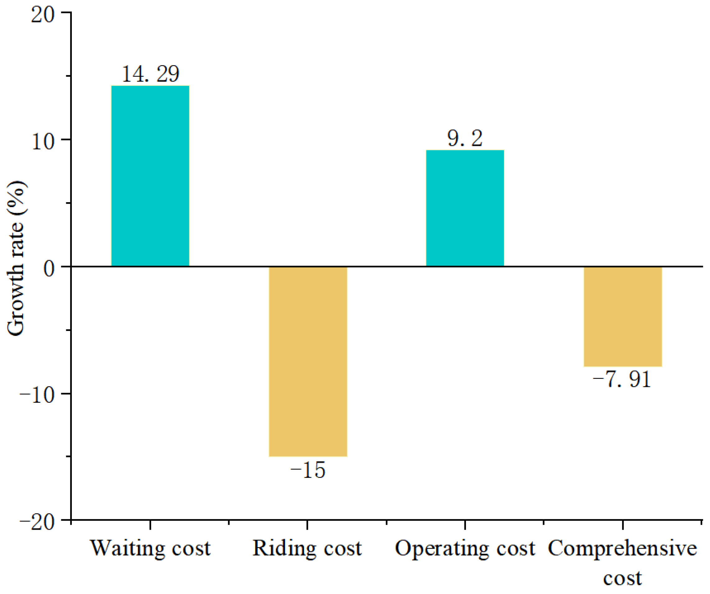
• The optimization model of bus scheduling under unbalanced conditions is studied. Taking the waiting cost, riding cost and operating cost of passengers as the comprehensive cost of the bus line, and taking the lowest comprehensive cost as the optimization objective, a two-way bus scheduling optimization model for peak passenger flow is established.
• A nonlinear inertia dynamic weight cuckoo search algorithm (DWCS) is proposed. Taking a bus line as a study example, the algorithm is used to solve the established scheduling optimization model. The results show that the scheduling optimization model established in this paper is 8.56% and 7.91% lower than that obtained using traditional single scheduling in the morning and evening, respectively.

However, this paper does not consider the allocation of bus resources between different stations and lines in the region, and the theoretical optimization results may be different from the actual operational results. Therefore, subsequent research on the optimization of bus scheduling needs to further consider the optimal allocation of transport capacity structures of different lines in the region and to allocate and integrate the transport capacity resources according to the actual operational capacity of bus enterprises.

References

1. Carey, M. Optimizing scheduled times allowing for behavioural response. Transp. Res. Part B Methodol. 1998, 32, 329–342. [Google Scholar] [CrossRef]
2. Hassold, S.; Ceder, A. Multiobjective Approach to Creating Bus Timetables with Multiple Vehicle Types. Transp. Res. Rec. J. Transp. Res. Board 2012, 2276, 56–62. [Google Scholar] [CrossRef]
3. Ceder, A. Optimal Multi-Vehicle Type Transit Timetabling and Vehicle Scheduling. Procedia-Soc. Behav. Sci. 2011, 20, 19–30. [Google Scholar] [CrossRef] [Green Version]
4. Chu, J.; Korsesthakarn, K.; Hsu, Y.T. Models and a solution algorithm for planning transfer synchronization of bus timetables. Transp. Res. Part E Logist. Transp. Rev. 2019, 131, 247–266. [Google Scholar] [CrossRef]
5. Takamatsu, M.; Taguchi, A. Bus Timetable Design to Ensure Smooth Transfers in Areas with Low-Frequency Public Transportation Services. Transp. Sci. 2020, 54, 1238–1250. [Google Scholar] [CrossRef]
6. Berrebi, S.J.; Watkins, K.E.; Laval, J.A. A real-time bus scheduling policy to minimize passenger wait on a high frequency route. Transp. Res. Part B Methodol. 2015, 81, 377–389. [Google Scholar] [CrossRef]
7. Gkiotsalitis, K. A model for the periodic optimization of bus scheduling times. Appl. Math. Model. 2020, 82, 785–801. [Google Scholar] [CrossRef]
8. Adamski, A. Optimal adaptive scheduling control in an integrated public transport management system. In Proceedings of the 2nd Meeting of the EURO Working Groupon Urban Traffic and Transportation, Paris, France, 15–17 September 1993; pp. 413–438. [Google Scholar]
9. HornM, E.T. Fleet scheduling and scheduling for demand-responsive passenger services. Transp. Res. Part C Emerg. Technol. 2002, 10, 35–63. [Google Scholar] [CrossRef]
10. Dakic, I.; Yang, K.; Menendez, M.; Chow, J.Y. On the design of an optimal flexible bus scheduling system with modular bus units: Using the three-dimensional macroscopic fundamental diagram. Transp. Res. Part B Methodol. 2021, 148, 38–59. [Google Scholar] [CrossRef]
11. Yang, X.; Liu, L. A Multi-Objective Bus Rapid Transit Energy Saving scheduling Optimization Considering Multiple Types of Vehicles. IEEE Access 2020, 8, 79459–79471. [Google Scholar] [CrossRef]
12. Zhang, H.; Zhao, S.; Liu, H.; Liang, S. Design of limited-stop service based on the degree of unbalance of passenger demand. PLoS ONE 2018, 13, e0193855. [Google Scholar] [CrossRef] [Green Version]
13. Luo, X.; Liu, Y.; Yu, Y.; Tang, J.; Li, W. Dynamic bus scheduling using multiple types of real-time information. Transp. B Transp. Dyn. 2019, 7, 519–545. [Google Scholar]
14. Huang, Z.; Li, Q.; Li, F.; Xia, J. A Novel Bus-scheduling Model Based on Passenger Flow and Arrival Time Prediction. IEEE Access 2019, 7, 106453–106465. [Google Scholar] [CrossRef]
15. Sun, F.; Wang, X.L.; Zhang, Y.; Liu, W.X.; Zhang, R.J. Analysis of Bus Trip Characteristic Analysis and Demand Forecasting Based on GA-NARX Neural Network Model. IEEE Access 2020, 8, 8812–8820. [Google Scholar] [CrossRef]
16. Laporte, G.; Ortega, F.A.; Pozo, M.A.; Puerto, J. Multi-objective integration of timetables, vehicle schedules and user routings in a transit network. Transp. Res. Part B Methodol. 2017, 98, 94–112. [Google Scholar] [CrossRef]
17. Hu, S.; Liang, Q.; Qian, H.; Weng, J.; Zhou, W.; Lin, P. Frequent-pattern growth algorithm based association rule mining method of public transport travel stability. Int. J. Sustain. Transp. 2021, 15, 879–892. [Google Scholar] [CrossRef]
18. Hadas, Y.; Shnaiderman, M. Public-transit frequency setting using minimum-cost approach with stochastic demand and travel time. Transp. Res. Part B Methodol. 2012, 46, 1068–1084. [Google Scholar] [CrossRef]
19. Tirachini, A.; Hensher, D.A. Bus congestion, optimal infrastructure investment and the choice of a fare collection system in dedicated bus corridors. Transp. Res. Part B Methodol. 2011, 45, 828–844. [Google Scholar] [CrossRef]
20. Fouilhoux, P.; Barra-Rojas, O.J.; Kedad-Sidhoum, S.; Rios-Solis, Y.A. Valid inequalities for the synchronization bus timetabling problem. Eur. J. Oper. Res. 2016, 251, 442–450. [Google Scholar] [CrossRef]
21. Yu, B.; Yang, Z.; Yao, J. Genetic algorithm for bus frequency optimization. J. Transp. Eng. 2010, 136, 576–583. [Google Scholar] [CrossRef]
22. Tang, J.; Yang, Y.; Qi, Y. A hybrid algorithm for urban transit schedule optimization. Phys. A Stat. Mech. Appl. 2018, 512, 745–755. [Google Scholar] [CrossRef]
23. Nam, K.; Park, M. Improvement of an optimal bus scheduling model based on transit smart card data in Seoul. Transport 2018, 33, 981–992. [Google Scholar] [CrossRef] [Green Version]
24. Jiang, M.; Zhang, Y.; Zhang, Y. Multi-Depot Electric Bus Scheduling Considering Operational Constraint and Partial Charging: A Case Study in Shenzhen, China. Sustainability 2021, 14, 255. [Google Scholar] [CrossRef]
Figure 1. Common types of bus stops: (a) bus station without bus bay and (b) harbor-shaped bus stop.
Sustainability 14 15839 g001
Figure 2. Three common bus scheduling forms.
Sustainability 14 15839 g002
Figure 3. DWCS algorithm flow.
Sustainability 14 15839 g003
Figure 4. Comparison of the standard test function seeking curve: (a) simple single-peaked function, (b) high-dimensional single-peaked function and (c) multi-peak function.
Sustainability 14 15839 g004
Figure 5. Time series of bus IC swipe card for a certain bus trip.
Sustainability 14 15839 g005
Figure 6. Inertia weighting graph.
Sustainability 14 15839 g006
Figure 7. Cost comparison of different scheduling modes in early peak hours.
Sustainability 14 15839 g007
Figure 8. Comparison of cost growth rates of different scheduling modes in early peak hours.
Sustainability 14 15839 g008
Figure 9. Cost comparison of different scheduling modes in the late peak hour.
Sustainability 14 15839 g009
Figure 10. Comparison of cost growth rates of different scheduling modes in the late peak hour.
Sustainability 14 15839 g010