Abstract
In order to promote scientific and technological innovation and sustainable development, public funding agencies select and fund a large number of R&D projects every year. To guarantee the performance of the resulting project portfolio and the government’s investment benefits, the decision maker needs to select appropriate projects and determine a reasonable funding amount for each selected project. In the process of project selection, it is necessary to consider the balance of funding allocated to different scientific sectors as well as the failure probability of the projects in future execution, so that the expected performance of the project portfolio is maximized as much as possible. In view of this, we propose and study the uncertain public R&D project portfolio selection problem considering sectoral balancing and project failure. We formulate a stochastic programming model for the problem to support the portfolio decisions of the funding agencies. We also transform the model into an equivalent deterministic second-order cone programming model that can be directly solved by exact solvers. We generate datasets reflecting different scenarios through simulation and perform computational experiments to validate our model. The impacts of various factors (i.e., the number of project proposals, project failure probability, the upper limit of the budget allocated to each project, and the decision maker’s tolerance for project failure) on the project portfolio performance are analyzed.
1. Introduction
Science and technology play a key role in socially sustainable development. Governments of various countries have invested a lot of money in the form of public R&D projects to promote scientific and technological innovation [1]. For example, the financial investment of the National Natural Science Foundation of China (NSFC) has increased from 80 million RMB in 1986 to 28 billion RMB in 2018 [2]; China’s total R&D investment reached 2786.4 billion RMB in 2021 [3]. The amount of capital investment received by each approved project has an impact on its performance, which in turn affects the effectiveness of government capital investment [4]. Since the total amount of funds available to the project funding agencies is limited, when the funding agencies fund R&D projects, they need to select a portfolio of projects with high potential from a large number of project proposals and allocate a reasonable budget for each selected project. As a result, the sustainability and efficiency of public funds are improved, and the project portfolio’s performance is maximized [5].
When the government funding agencies select the portfolio of R&D projects, it is necessary to ensure the balance of budget allocation among different sectors or scientific disciplines, such that a certain degree of fairness is ensured. Typical ways of balancing budget allocation include limiting the proportion or amount of funds allocated to different sectors [6,7] and limiting the number of projects funded in different sectors [8]. Karsu and Morton propose an imbalance indicator that measures the difference of a distribution from an ideally balanced distribution and define a bi-criteria framework for trading balance off against efficiency in resource allocation problems [9]. However, these studies are based on the assumption that the decision maker knows the optimal balanced allocation results. In practice, it is also difficult for the decision maker to determine the balanced allocation in advance. Çağlar and Gürel propose a two-stage model in which they make sectoral budget allocation decisions in the first stage to maximize the total impact of the budget while ensuring the relative balance among sectors, and in the second stage they maximize the total score of the supported projects under allocated sectoral budgets [10]. Both Mavrotas and Özpeynirci et al. develop interactive approaches that require the decision maker to perform pairwise comparisons among alternative allocation schemes [11,12]. In addition, the budget allocation can also be improved from the perspective of project resource allocation by using the fuzzy sets theory [13,14,15].
The projects are selected before they are executed, and some of the selected projects may fail during the long time period from the fund allocation to their completion. Therefore, when constructing the project portfolio, the government funding agencies may benefit from considering the probability of different projects failing in the future. In fact, in the project environment, researchers have developed many methods to estimate different types of likelihood [16]. For example, Kahraman and İhsan employ the concept of probability of a fuzzy event to perform investment analysis [17]. Fuzzy numbers are used to model uncertain activity times and their distributions [18,19]. Balali et al. use artificial neural networks to predict the cost performance indices of a project [20]. In the field of public R&D project portfolio selection, only a few studies have considered project failure. To solve a public R&D project portfolio selection problem with cancellations, Çağlar and Gürel develop a robust optimization model for the case that the cancellation probabilities are unknown, and a stochastic optimization model for the case that the cancellation probabilities can be assessed [21]. Mohagheghi et al. propose project resilience as a key criterion in the large-scale construction project selection problem [22]. Gouglas and Marsh study the optimal portfolio solutions of the vaccine technologies by estimating their probability of success for rapid response to emerging infections [23]. Some studies also consider project failure in the private R&D project portfolio selection field. Zhao et al. build a mixed-integer nonlinear programming model to maximize the expected net present value for the selection of projects under variable task failures [24]. Gökalp and Branke consider a pharmaceutical R&D pipeline management problem under two significant uncertainties, i.e., the outcomes of clinical trials and their durations, and they present an approximate dynamic programming approach to solve the problem [25]. Tamošaitienė et al. discover that project risks might cause firms to end up facing big losses or even failure, hence they use the risk and return trade-off in choosing their portfolios of projects [26].
In addition, in the field of project portfolio selection, whether it takes public or private R&D projects as the research object, there are many studies that consider the interrelationships and interactions between projects. There are often substitutional or complementary relationships between some projects, and the outcomes or technologies of the projects influence each other. The interrelationships make the performance of the project portfolio a nonlinear function of the selected projects and further increase the complexity of the R&D portfolio selection. In the field of public project portfolio selection, Fernandez et al. consider the interactions and synergies between projects and the decision maker’s preferences when solving the problem of allocating public funds to competing programs or projects [27]. Arratia-Martinez et al. take into account portfolio balancing rules and interdependence between tasks and/or projects and solve the R&D project portfolio selection problem under uncertainty [28]. Wei et al. construct a co-citation network to simulate project interactions and study the ways in which project interactions influence the final values of project portfolios [29]. Delouyi et al. use network mapping to visualize project interdependencies and improve the quality of the dynamic portfolio selection decision in cross-country gas transmission projects [30]. In the private project portfolio selection field, both Pérez et al. and Kumar et al. believe that uncertain synergies and incompatibilities exist between projects, and they handle these uncertainties using fuzzy parameters [31,32]. Ghasemi et al. believe project interdependencies and cause–effect relationships between risks create complexity for portfolio risk analysis, so they present a model using a Bayesian network for modeling and analyzing portfolio risks [33].
Therefore, in project portfolio selection, there are relatively few studies on public R&D projects. Table 1 summarizes the representative studies mentioned above. It can be seen that, both in deterministic and uncertain environments, no research has yet considered sectoral balancing and project failure. This paper aims to fill this gap. The main contributions of this paper are as follows: (1) We propose and study the uncertain public R&D project portfolio selection problem, considering both sectoral balancing and project failure (URDPS). (2) We formulate a stochastic programming model for the URDPS. We then transform the stochastic programming model into an equivalent deterministic second-order cone programming model such that it can be solved by commercial solvers (e.g., CPLEX). (3) We perform computational experiments to validate our model and analyze the impacts of the number of project proposals, project failure probability, the upper limit of the budget allocated to each project, and the decision maker’s tolerance for project failure on the portfolio performance.

Table 1.
Representative studies in project portfolio selection.
The remainder of this article is structured as follows. In Section 2, we describe the uncertain public R&D project portfolio selection problem considering both sectoral balancing and project failure. Section 3 presents the stochastic optimization model and its equivalent deterministic second-order cone programming model. In Section 4, we analyze our model based on computational experiments. Section 5 offers conclusions and suggestions for future work.
2. Problem Statement
The funding organization receives project proposals () and needs to select a subset of the projects to fund. The selected projects form a portfolio. There are sectors, and each project belongs to a single sector. For example, the NSFC’s funding covers nine sectors. Let denote the set of project proposals under sector . The funding organization has a budget 𝐵. The variable represents the budget for sector , . is not greater than the sum of the required budgets for all project proposals, i.e., . There are sectors whose numbers of funded projects are limited to the interval . Let denote the set of project proposals in this type of sector (.
Peer reviewers assess each project proposal and assign a score for . If is lower than a pre-given threshold, project will not be funded. If is not lower than the threshold, the decision maker of the funding organization needs to further determine the actual fund allocated to project . We use to denote the proportion of the actual allocated fund to the fund claimed by the principal investigator, which is also used as an estimation for the future expected performance after project is finished. Therefore, the actual obtained fund for project is and it has an upper limit of . In addition, to ensure that project is funded enough to be executed, we provide a lower limit to . For the convenience of subsequent modeling, we also introduce an auxiliary variable to indicate whether project is funded or not: if , then let ; otherwise let . It can be seen that the nonzero elements in the set correspond to a project portfolio.
To ensure fairness, the funding organization considers sectoral balancing when selecting projects. A proper capital allocation [14] is essential for balancing the budget allocation. Sectoral balancing avoids situations where some sectors receive most of the funds and others receive little. We quantify the balance of budget allocation based on each sector’s historical contribution and impact () on society [10]. It is a trend in public R&D funding to assess the impact of each sector’s outcomes and decide the budget allocation accordingly. For example, Graham and Mackie shift 3.4% of the agency budget from lower-impact areas to higher-impact areas, which improves the public health impact of the resources [34]. Following Çağlar and Gürel [10], the impact of a portfolio is calculated as , where represents the disfavor of funding agencies to the inequities that result from disparate budgets across disciplines. For a given , the maximum value of can be obtained by solving the following nonlinear programming model [10]:
It is not uncommon for a project to be faced with uncertainties [13,17]. In our problem, due to the uncertainty of scientific research, each project has a probability of failure when executed in the future. If project fails, the actual budget used is , where is the proportion of the funds used at the time of failure to its grant amount. Let random variable denote the actual budget used by project in its future execution, then we obtain
The funding organization wants to limit the number of failed projects in the portfolio, so the total number of failed projects should not exceed , where is set by the funding agency according to its needs and determines the maximum expected number of failed projects.
There are different relationships between projects. The relationships have different impacts on the ultimate performance of the corresponding portfolio. For example, co-funding complementary projects helps to increase the expected performance of the portfolio, whereas co-funding competing projects tends to decrease the expected performance of the portfolio. We consider the two types of relationships mentioned above when constructing the project portfolio. When the interrelated projects and are chosen simultaneously, the additional impact on the total score of the project portfolio is expressed as . When , it means that the selection of both projects and has a positive impact on the portfolio performance; otherwise, there is a negative impact. Due to the existence of the project failure probability, the expected additional impact of projects and on the total score of the project portfolio is .
The public R&D project portfolio selection problem studied in this paper aims at constructing a portfolio with the maximum expected total score of the project portfolio while considering sectoral balancing, project failure, and project interrelationships. We express as , where is the expected total score under the condition of project failure without considering project interrelationships, is the added value of the expected score of the portfolio caused by the interrelationships between the projects, and is the set of all possible pairwise projects with interrelationships.
3. Optimization Models
3.1. Stochastic Programming Model
We formulate the following stochastic programming model (SP) for the above problem:
:
(2)–(4).
Constraints on the number of funded projects:
Constraints on the funding proportion:
Funding amount constraints:
Sectoral balancing constraints:
Chance constraints on budget:
Constraints on the number of failed projects:
Range of decision variables:
In model SP, the objective function (6) maximizes the expected total score of the portfolio. Constraints (7) and (8) restrict the lower and upper limits of the number of funded projects in different sectors, respectively. Constraints (9) express the logical relations between decision variables and . Constraints (10) indicate the lower limit of the funding proportion for each project. Constraints (11) are the upper limit for the funded amount of each project. Constraint (12) ensures that the degree of balance in budget allocation between sectors is not less than , where the balancing preference parameter reflects the degree to which the funding organization wants the balance of the budget allocation to reach its theoretical maximum value . Chance Constraints (13) ensure that when the project is executed, the probability that the budget of each sector does not exceed the planned quota is greater than or equal to the confidence level . Constraint (14) limits the number of failed projects. Finally, Constraints (15) and (16) define the range of the decision variables.
It should be noted that both Constraints (12) and (13) in SP are nonlinear. Therefore, SP is a nonlinear optimization model. To solve the model with exact solvers (e.g., CPLEX), we will transform SP into its equivalent deterministic second-order cone programming model in the next subsection.
3.2. Second-Order Cone Programming Model
By introducing auxiliary variables and second-order cone inequalities, we transform SP into an equivalent deterministic second-order cone programming model. First, proposition 1 transforms the nonlinear constraints in (13) into deterministic second-order cone constraints.
Proposition 1.
The constraints in (13) are equivalent to the following constraints:
Proof.
The expectation of is . The variance of is .
Based on the properties of the normal distribution, the chance constraints in (13) can be transformed into Constraints (20), where denotes the cumulative distribution function of the normal distribution:
Let denote the inverse function of . Since is monotonically increasing, constraints (20) can be further transformed into the following constraints:
We then obtain Constraints (22) by plugging the expectation and variance into Constraints (21):
Since , Constraints (22) are convex and equivalent to Constraints (17)–(19), where Constraints (18) are second-order cone constraints and is a continuous auxiliary variable. □
Next, proposition 2 transforms the nonlinear constraint in (12) into the equivalent Constraints (23)–(27).
Proposition 2.
Model SP is equivalent to model MISOCP:
(MISOCP) Maximize (6)
Subject to
(2)–(4), (7)–(11), (14)–(19)
Proof.
In Constraint (12), can be replaced by two positive integers and , i.e., . Then Constraint (12) can be converted to Constraint (28):
By introducing an auxiliary variable , Constraint (28) can be split into Constraints (23) and (29):
where Constraint (23) is linear and Constraints (29) are nonlinear. We need to further transform Constraints (29) that are equivalent to the following constraints:
There exist positive integers and that satisfy . We can transform Constraints (30) into Constraints (31):
Following Çağlar and Gürel [10], we set . In this case, . We substitute the values of and into Constraints (29) and obtain Constraints (32) based on Constraints (29)–(31).
Alzalg [35] shows that for any inequality of the form , if , then the inequality can be expressed by at most inequalities of the form , where . Based on this, we transform Constraints (32) into a set of inequalities (33)–(35). Constraints (27) specify the range of the auxiliary variables and .
For any inequality of the form , it can be converted to conic quadratic inequality . Therefore, the inequality set (33)–(35) can be further transformed into the conic quadratic inequality set (24)–(26). □
MISOCP is a mixed-integer second-order cone program that can be directly solved by CPLEX.
4. Computational Experiments
In this section, we investigate the following four research questions (RQs) based on computational experiments.
RQ1: How does the number of project proposals affect the total score of the portfolio?
RQ2: The failure probability of a project affects the chance of the project being selected. Then, how does the proportion of projects with high and low failure probability in all candidate projects affect the portfolio performance?
RQ3: How do different upper limits of the budget allocated to each project affect the performance of the project portfolio?
RQ4: The decision maker’s tolerance for project failure affects the chance of a project being selected. Then, how do different failure tolerances affect the portfolio performance?
In our experiments, the above RQs are answered by solving the MISOCP model with CPLEX. Our code is programmed in MATLAB 2016a, and CPLEX is also called by MATLAB 2016a. Our experiments were conducted on a computer equipped with a Ryzen5 5500U 2.1 GHz CPU and Windows 11 64-bit.
4.1. Benchmark Dataset
There is no dataset designed specifically for our problem. Therefore, we generate the benchmark dataset SET using a full factorial design. We call the situation corresponding to the benchmark dataset the baseline scenario. The parameter values of the benchmark dataset are shown in Table 2. For each parameter combination in Table 2, 10 instances are generated. Since each parameter in Table 2 has only one value, this leads to 10 instances in the benchmark dataset. The dataset used in this paper has been uploaded to https://github.com/RuiChen-329/URDPS, accessed on 18 October 2022.
Table 2.
Parameter values for the benchmark dataset .
4.2. Performance Measure
In our experiments, we generate multiple variants of the baseline scenario by changing the parameter values in the baseline scenario. The number of instances contained in each scenario variant is the same as the number of instances in the baseline scenario. Based on the computational results obtained by comparing the scenario variants with the baseline scenario, we answer the four RQs. In the comparisons, we use the average relative deviation (ARD) of the total score as the performance measure. ARD measures the average gap in the optimal objective function value between the scenario variants and the baseline scenario. ARD is calculated as follows:
where ( is the optimal objective function value of instance in the scenario variants (baseline scenario). The value of the ARD reveals the impacts of the factors (i.e., the number of project proposals, the funding amount, and the decision maker’s tolerance for project failure) on the performance of the project portfolio. In other words, when the decision maker chooses an alternative scenario instead of the baseline scenario, the value of the ARD indicates the gain or loss of the decision. The smaller the ARD value, the weaker the impact of the factors on the portfolio selection result.
When using CPLEX to solve each instance in different scenarios, we set the time limit to 30 s. The results show that 180 out of the 410 instances are solved to optimality. For the remaining 230 instances, only feasible solutions are obtained, and the estimated optimality gaps given by CPLEX are within 0.02%.
4.3. Experimental Results
We perform four experiments to answer the four RQs, respectively. As shown in Table 3, in each experiment, only one parameter’s value is changed compared to the baseline scenario, and we generate 10 scenario variants (other parameters are kept unchanged). Note that in Experiment 2, instances of scenario variants 1–5 and 6–10 are obtained by extracting the failure probabilities of 10–50% of the baseline scenario instances from the intervals (0, 0.1) and (0.2, 0.3), respectively.
Table 3.
Parameter values for the scenario variants.
The computational results are shown in Figure 1. We can see from Figure 1 that the number of project proposals, the upper limit of the budget allocated to each project, and the decision maker’s tolerance for project failure have positive impacts on the portfolio performance. This means that the greater the values of these parameters, the higher the performance of the project portfolio. For the number of project proposals, this result is obvious: more candidate projects tend to contain more potential projects that can contribute more to the portfolio. In addition, the impact of the number of project proposals is linear.
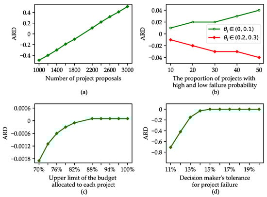
Figure 1.
The impacts of different parameters on the portfolio performance.
The impacts of the upper limit of the budget allocated to each project and the decision maker’s tolerance for project failure are non-linear and follow a similar pattern. Specifically, before the thresholds (88% for the former factor and 14% for the latter) are reached, the performance of the portfolio increases rapidly as the above two factors increase. After the thresholds are reached, the impacts of both factors become steady. This means that for the upper limit of the budget allocated to each project, after most of the selected projects are allocated to large enough funds, increasing the funding amount of each project benefits fewer. For the decision maker’s tolerance for project failure, it reveals that the number of failed projects should be controlled within a certain range, which can achieve higher portfolio performance.
Compared with the baseline scenario, when the probability of project failure is small (large), the performance of the project portfolio is higher (lower). Increasing the number of projects with a low failure probability helps enhance the portfolio performance.
5. Conclusions and Future Research
In this paper, considering sectoral balancing, project failure probability, and interrelationships between projects, we have studied the uncertain public R&D project portfolio selection problem to maximize the expected performance of the project portfolio. We formulate a stochastic programming model for the problem. We transform the stochastic programming model into an equivalent deterministic second-order cone programming model that can be directly solved by exact solvers. Computational experiments are conducted to analyze the impacts of different factors on the project portfolio performance. The results show that the number of project proposals, the funding amount, and the decision maker’s tolerance for project failure have positive impacts on the portfolio performance, whereas the probability of project failure has a negative impact.
Our results reveal that the proposed method provides an effective tool to aid the decision maker’s project portfolio selection decisions. By incorporating real-world characteristics that appear in public R&D project portfolio selection such as sectoral balancing, project failure, and project interrelationships, our method is able to generate satisfactory project portfolios for different decision scenarios. Our method is easily embeddable into funding agency information systems, resulting in portfolio selection solutions that are automatically obtained to serve as a reference for decision-making and the effective utilization of public investment.
Future work will consider more factors in public R&D portfolio selection, such as the robustness of the solution. Additionally, since project funding agencies make project selection decisions dynamically or at regular intervals, it is necessary to study the problem from the perspective of a multi-stage decision-making process.
Author Contributions
Conceptualization, H.L.; methodology, H.L. and R.C.; software, H.L. and R.C.; validation, H.L. and R.C.; formal analysis, H.L. and R.C.; investigation, H.L. and R.C.; resources, H.L., R.C. and X.Z.; writing—original draft preparation, H.L. and R.C.; writing—review and editing, H.L., R.C. and X.Z.; visualization, H.L. and R.C.; supervision, H.L.; project administration, H.L.; funding acquisition, H.L. and X.Z. All authors have read and agreed to the published version of the manuscript.
Funding
This research was funded by the National Social Science Fund of China (Grant Number 21&ZD131).
Institutional Review Board Statement
Not applicable.
Informed Consent Statement
Not applicable.
Data Availability Statement
Publicly available datasets were analyzed in this study. This data can be found here: https://github.com/RuiChen-329/URDPS, accessed on 18 October 2022.
Conflicts of Interest
The authors declare no conflict of interest.
References
- Li, H.; Yao, B.; Yan, X. Data-Driven Public R&D Project Performance Evaluation: Results from China. Sustainability 2021, 13, 7147. [Google Scholar] [CrossRef]
- NSFC. Investment in the National Natural Science Foundation of China Has Increased 300-Fold over the Past 30 Years. Available online: https://www.nsfc.gov.cn/publish/portal0/tab440/info55794.htm (accessed on 22 August 2022).
- China.org.cn China’s R&D Investment Intensity Hit a New High in 2021. Available online: http://www.gov.cn/xinwen/2022-01/27/content_5670659.htm (accessed on 22 August 2022).
- Dobrzanski, P.; Bobowski, S. The Efficiency of R&D Expenditures in ASEAN Countries. Sustainability 2020, 12, 2686. [Google Scholar] [CrossRef]
- Kim, E.S.; Choi, Y.; Byun, J. Big Data Analytics in Government: Improving Decision Making for R&D Investment in Korean SMEs. Sustainability 2020, 12, 202. [Google Scholar] [CrossRef]
- Beaujon, G.J.; Marin, S.P.; McDonald, G.C. Balancing and Optimizing a Portfolio of R&D Projects. Nav. Res. Logist. 2001, 48, 18–40. [Google Scholar] [CrossRef]
- Litvinchev, I.S.; López, F.; Alvarez, A.; Fernandez, E. Large-Scale Public R&D Portfolio Selection by Maximizing a Biobjective Impact Measure. IEEE Trans. Syst. Man Cybern.—Part A Syst. Hum. 2010, 40, 572–582. [Google Scholar] [CrossRef]
- Mavrotas, G.; Diakoulaki, D.; Caloghirou, Y. Project Prioritization under Policy Restrictions. A Combination of MCDA with 0–1 Programming. Eur. J. Oper. Res. 2006, 171, 296–308. [Google Scholar] [CrossRef]
- Karsu, Ö.; Morton, A. Incorporating Balance Concerns in Resource Allocation Decisions: A Bi-Criteria Modelling Approach. Omega 2014, 44, 70–82. [Google Scholar] [CrossRef][Green Version]
- Çağlar, M.; Gürel, S. Impact Assessment Based Sectoral Balancing in Public R&D Project Portfolio Selection. Socio-Econ. Plan. Sci. 2019, 66, 68–81. [Google Scholar] [CrossRef]
- Mavrotas, G.; Makryvelios, E. Combining Multiple Criteria Analysis, Mathematical Programming and Monte Carlo Simulation to Tackle Uncertainty in Research and Development Project Portfolio Selection: A Case Study from Greece. Eur. J. Oper. Res. 2021, 291, 794–806. [Google Scholar] [CrossRef]
- Özpeynirci, S.; Özpeynirci, Ö.; Mousseau, V. An Interactive Algorithm for Resource Allocation with Balance Concerns. OR Spectr. 2021, 43, 983–1005. [Google Scholar] [CrossRef]
- Rola, P.; Kuchta, D. Application of Fuzzy Sets to the Expert Estimation of Scrum-Based Projects. Symmetry 2019, 11, 1032. [Google Scholar] [CrossRef]
- Chrysafis, K.A.; Papadopoulos, B.K. Decision Making for Project Appraisal in Uncertain Environments: A Fuzzy-Possibilistic Approach of the Expanded NPV Method. Symmetry 2021, 13, 27. [Google Scholar] [CrossRef]
- Lyczkowska-Hanckowiak, A. On Application Oriented Fuzzy Numbers for Imprecise Investment Recommendations. Symmetry 2022, 12, 1627. [Google Scholar] [CrossRef]
- Ahmadi, E.; McLellan, B.; Ogata, S.; Mohammadi-Ivatloo, B.; Tezuka, T. An Integrated Planning Framework for Sustainable Water and Energy Supply. Sustainability 2020, 12, 4295. [Google Scholar] [CrossRef]
- Kahraman, C.; Kaya, I. Investment Analyzes Using Fuzzy Probability Concept. Technol. Econ. Dev. Econ. 2010, 16, 43–57. [Google Scholar] [CrossRef]
- Chrysafis, K.A.; Panagiotakopoulos, D.; Papadopoulos, B.K. Hybrid (Fuzzy-Stochastic) Modelling in Construction Operations Management. Int. J. Mach. Learn. Cybern. 2013, 4, 339–346. [Google Scholar] [CrossRef]
- Chrysafis, K.A.; Papadopoulos, B.K. Approaching Activity Duration in PERT by Means of Fuzzy Sets Theory and Statistics. J. Intell. Fuzzy Syst. 2014, 26, 577–587. [Google Scholar] [CrossRef]
- Balali, A.; Valipour, A.; Antucheviciene, J.; Saparauskas, J. Improving the Results of the Earned Value Management Technique Using Artificial Neural Networks in Construction Projects. Symmetry 2020, 12, 1745. [Google Scholar] [CrossRef]
- Çağlar, M.; Gürel, S. Public R&D Project Portfolio Selection Problem with Cancellations. OR Spectr. 2017, 39, 659–687. [Google Scholar] [CrossRef]
- Mohagheghi, V.; Mousavi, S.M.; Mojtahedi, M.; Newton, S. Introducing a Multi-Criteria Evaluation Method Using Pythagorean Fuzzy Sets: A Case Study Focusing on Resilient Construction Project Selection. Kybernetes 2020, 50, 118–146. [Google Scholar] [CrossRef]
- Gouglas, D.; Marsh, K. Prioritizing Investments in Rapid Response Vaccine Technologies for Emerging Infections: A Portfolio Decision Analysis. PLoS ONE 2021, 16, e0246235. [Google Scholar] [CrossRef]
- Zhao, W.; Hall, N.G.; Liu, Z. Project Evaluation and Selection with Task Failures. Prod. Oper. Manag. 2020, 29, 428–446. [Google Scholar] [CrossRef]
- Gökalp, E.; Branke, J. Pharmaceutical R & D Pipeline Management under Trial Duration Uncertainty. Comput. Chem. Eng. 2020, 136, 106782. [Google Scholar] [CrossRef]
- Tamošaitienė, J.; Yousefi, V.; Tabasi, H. Project Portfolio Construction Using Extreme Value Theory. Sustainability 2021, 13, 855. [Google Scholar] [CrossRef]
- Fernandez, E.; Lopez, E.; Mazcorro, G.; Olmedo, R.; Coello Coello, C.A. Application of the Non-Outranked Sorting Genetic Algorithm to Public Project Portfolio Selection. Inf. Sci. 2013, 228, 131–149. [Google Scholar] [CrossRef]
- Arratia-Martinez, N.M.; Caballero-Fernandez, R.; Litvinchev, I.; Lopez-Irarragorri, F. Research and Development Project Portfolio Selection under Uncertainty. J. Ambient. Intell. Humaniz. Comput. 2018, 9, 857–866. [Google Scholar] [CrossRef]
- Wei, H.; Niu, C.; Xia, B.; Dou, Y.; Hu, X. A Refined Selection Method for Project Portfolio Optimization Considering Project Interactions. Expert Syst. Appl. 2020, 142, 112952. [Google Scholar] [CrossRef]
- Delouyi, F.L.; Ghodsypour, S.H.; Ashrafi, M. Dynamic Portfolio Selection in Gas Transmission Projects Considering Sustainable Strategic Alignment and Project Interdependencies through Value Analysis. Sustainability 2021, 13, 5584. [Google Scholar] [CrossRef]
- Pérez, F.; Gómez, T.; Caballero, R.; Liern, V. Project Portfolio Selection and Planning with Fuzzy Constraints. Technol. Forecast. Soc. Change 2018, 131, 117–129. [Google Scholar] [CrossRef]
- Kumar, M.; Mittal, M.L.; Soni, G.; Joshi, D. A Hybrid TLBO-TS Algorithm for Integrated Selection and Scheduling of Projects. Comput. Ind. Eng. 2018, 119, 121–130. [Google Scholar] [CrossRef]
- Ghasemi, F.; Sari, M.H.M.; Yousefi, V.; Falsafi, R.; Tamošaitienė, J. Project Portfolio Risk Identification and Analysis, Considering Project Risk Interactions and Using Bayesian Networks. Sustainability 2018, 10, 1609. [Google Scholar] [CrossRef]
- Graham, J.R.; Mackie, C. Criteria-Based Resource Allocation: A Tool to Improve Public Health Impact. J. Public Health Manag. Pract. 2016, 22, E14. [Google Scholar] [CrossRef] [PubMed]
- Alzalg, B.M. Stochastic Second-Order Cone Programming: Applications Models. Appl. Math. Model. 2012, 36, 5122–5134. [Google Scholar] [CrossRef]

Publisher’s Note: MDPI stays neutral with regard to jurisdictional claims in published maps and institutional affiliations. |
© 2022 by the authors. Licensee MDPI, Basel, Switzerland. This article is an open access article distributed under the terms and conditions of the Creative Commons Attribution (CC BY) license (https://creativecommons.org/licenses/by/4.0/).