Abstract
Lightweight structures built on expansive soils are susceptible to damage caused by soil movement. Financial losses resulting from the improper design of structures on expansive soils can be significant. The interactions and failure mechanisms of different geotechnical structures constructed on such soils differ depending on the structure type, site characteristics, and climatic conditions, as the behaviour of expansive soils is influenced by moisture variations. Therefore, the performance of different geotechnical structures (e.g., lightweight footings for residential buildings) is expected to be adversely affected by climate change (especially rainfall and temperature change), as geotechnical structures are often designed to have a service life of 50–100 years. Some structures may even fail if the effect of climate change is not considered in the present design. This review aims to provide insights into problems associated with expansive soils that trigger the failure of lightweight structures, including current investigations and industry practices. This review recognises that although the soil moisture conditions govern expansive soil behaviour, limited studies have incorporated the effect of future climate changes. In addition, this review identifies the need to improve the current Australian design practice for residential footings through the inclusion of more site-specific investigations and expected climate changes.
1. Introduction
Expansive soils, also referred to as reactive soils, can be found all over the world, in arid or semi-arid zones with tropical or temperate climates [1]. Koukouzas et al. [2] defined expansive soil as soil that undergoes a significant volume change due to changes in water content, resulting in ground movement. They contain minerals of Kaolinite, Montmorillonite and Illite groups. The functionalities of geo-infrastructure, such as pavements, pipelines, and shallow footings, located on expansive soil may be affected due to ground movement brought in by moisture content changes. From a financial perspective, expansive soils are considered a significant contributor to damage, with billions of dollars in losses every year [3]. For instance, the annual cost of damage to buildings and infrastructure due to soil shrinkage-induced subsidence is estimated to exceed USD 15 billion in the US alone [4]. The repair cost for damages to structures associated with expansive soil has been projected to be double the total due to the cumulative damage from natural disasters in the US [5]. Similarly, 80% of the total annual housing insurance claims in Australia are attributed to approximately 50,000 housing cracks caused by soil movement [6]. In the state of Victoria alone, housing defects cost nearly AUD 1 billion per year, with the majority being footing and slab defects [7]. The extended dry weather period between 1997 and 2010 affected much of Australia, including the greater Melbourne area. According to an estimate by the Housing Industry Association, more than 1000 houses built in the dry seasons during a decade-long drought in the western suburbs of Melbourne were damaged as a result of excessive soil heave [8]. Another estimate suggested that the number of properties affected may be as high as 4300 [9]. Larger-than-expected ground movements were observed after the long drought broke in 2011 and were amplified by the construction of gardens/lawns and watering systems around buildings [10]. These damages and related consequences were likely due to underestimation of the ground movement potential.
The climate in Australia and around the world will continue to change in the coming decades, leading to significant socio-economic impacts [11]. Accounting for all climate variables can be a complex exercise, and changes in rainfall and temperature have been considered as the primary variables in most studies that investigated the soil–atmospheric boundary interaction, especially the ones looking at the effect of climate change [12,13,14,15,16,17]. Changes in temperature and rainfall may affect the behaviour of geotechnical infrastructure. Moreover, changes such as rises in the sea level, changes in soil suction profiles resulting from changes in precipitation patterns, excessive desiccation due to prolonged spells of high-temperature days, soil erosion, hydro-mechanical failure resulting from rising water pressure inside soils [18], slope stability changes [12,17,19,20,21,22,23,24,25,26,27,28,29,30], and changes in the strength and stiffness of pavement materials [31] can affect geotechnical infrastructure. Depending on the geolocation, local climate, expected future changes in the climate, and structure type, these effects can vary. Although soil–atmospheric boundary interactions have been an active area of research over the last two decades, limited attention has been paid to reactive soil movement and its interaction with structures [16]. This problem is likely to worsen because of climate change.
Although the engineering properties of expansive soils can be improved by various techniques [32,33,34,35,36,37,38,39,40], to ensure safer, more resilient, and sustainable designs of geotechnical structures, it is vital to better understand the interactions among expansive soils, atmospheric boundaries, vegetations (if present), and structures. Hence, this review aims to explore different factors that affect the performance of lightweight structures built on expansive soils, highlighting the extent of the problems and the state of the art in current research and industry practice.
Some aspects of the behaviour of expansive soils are discussed in the next section, followed by a discussion of different application areas with potential problems. Various investigations (laboratory, field, and numerical) of soil–atmospheric interactions considering structural performance are explored. Current industry practices for dealing with expansive soils are discussed in Section 5, with an example of the Australian design practice for residential footings and pavements. This review aims to familiarise readers with the basic mechanism of existing problems facing structures on expansive soils, the current state of understanding, and an Australian practice to facilitate the development of further research to better address the current issues.
2. Expansive Soil Behaviour
Expansive soil expands when its degree of saturation increases, i.e., with an increase in moisture content, and it shrinks when moisture is removed. The existence of expansive soils can be identified through deeper cracks with roughly polygonal shapes on the ground surface during the dry season [41]. In the rainy season, water enters through these cracks, and the soil expands, which may cause the cracks to disappear. The presence of different types of clay minerals is responsible for this behaviour. The expansiveness of soil increases with the presence of clay minerals in the order of Kaolinite, Illite, Vermiculite, and Montmorillonite. Montmorillonite is the most expansive mineral, with the highest activity and Atterberg limits, whereas Kaolinite is the least expansive mineral, with the lowest values of these parameters [42,43]. Furthermore, the bond between various building blocks, as shown in Figure 1, plays a vital role in the behaviour of minerals. In Kaolinite, strong bonds exist between the top of the silica and octahedral sheets (Figure 1a), as the replacement of oxygen atoms and hydroxyls can occur between the top of the silica tetrahedra and octahedral sheets, respectively [44]. However, Montmorillonite has the weakest bond because of the very weak bonding between two bases of the silica sheets (Figure 1c), resulting in a thickness of one to two groups of building blocks. Illite has the same structure as Montmorillonite (Figure 1b), except for the bond created by the potassium cations between the bases of the sheets, which produces stronger bonds. This bonding dictates the expansion and contraction potential of the soil. In minerals with weak bonds, water can move in and out easily, which leads to expansion or contraction due to the hydration or dehydration of clay minerals. However, a strong bond does (e.g., Kaolinite) not allow much water flow and less soil movement is expected.
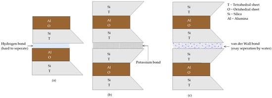
Figure 1.
Schematic representation of mineral structures: (a) Kaolinite; (b) Illite; (c) Montmorillonite, adapted from Nelson et al. [44].
In general, near-surface soil undergoes seasonal moisture changes that contribute to ground movement. Beyond a certain depth, the changes in water content and related changes in matric suction become very small and thus do not contribute to movement [45]. The zone subject to seasonal moisture changes can be expected to extend from depths of 0.9 to 12 m [41]. Any structures constructed on or within the depth where seasonal moisture changes occur are likely to be subjected to additional stresses due to ground movement.
3. Problems with Expansive Soils
Lightweight buildings, pipelines, pavements, and other shallow services such as sewer manholes and pylons can be considered lightweight structures, and these structures are found to be most affected by expansive soils [46]. Soil can produce significant uplift pressure during swelling (as much as 250 kPa) [41]. For heavier structures such as high-rise buildings, their dead weight is often sufficiently large to counteract and suppress any effect of this swelling pressure. Table 1 summarises the common problems associated with expansive soil movement.

Table 1.
Common problems related to expansive soil movement.
Cyclic shrink–swell movement due to seasonal changes in moisture content can lead to various damage to infrastructure. Owing to changes in moisture dynamics due to the construction of the structure and natural heterogeneity of the soil, movement does not occur uniformly. For example, in the dry part of the year, the edges of a building footing may have significantly lower moisture content than the centre of the footing, leading to centre heave, which can lead to substantial damage to the superstructure, as shown in Figure 2b. The opposite can occur in the wet season, when the edges of the footing have higher water content than the centre and differential stresses are applied to the footing and superstructure (see Figure 2a).
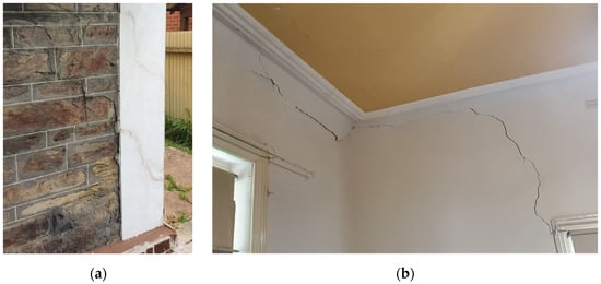
Figure 2.
Damage to a building (a) due to edge heave; (b) due to centre heave.
Figure 3 shows the road failure mechanism in soils susceptible to the shrink–swell phenomenon. Evapotranspiration can occur from the uncovered road edges, whereas it cannot occur from the covered road surface. This results in dry conditions at the edges of the road and wetter conditions toward the centre line of the road. The opposite trend can occur during the wet period of the year. This leads to settlement/heaving at the road edges, resulting in the formation of longitudinal cracks. In addition, road surface undulating also results from soil’s shrink–swell movement.
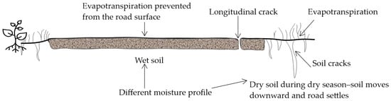
Figure 3.
Soil–atmosphere interactions on a road resulting in longitudinal crack formation.
The pipe–soil interaction due to moisture variation near a driveway is shown in Figure 4. In the dry season, owing to soil shrinkage, pipes may bend downward (Figure 4a), creating tensile strain on the soil mass above the pipe owing to the interaction between the pipe and soil. In contrast, in the wet season, the soil below the pipe expands, resulting in upward bending of the pipe (Figure 4b), thereby developing a compressive strain on the soil mass above the pipe. From field monitoring of buried flexible pipes, Clayton et al. [47] observed considerable ground movement (3–6 mm/m pipe length) due to the effect of underlying soil desiccation. Their simulation of the effect of this ground movement on cast iron pipe behaviour showed a significant increase in tensile stress, which could contribute to the failure of the pipe. Hence, a reduction in pipe strength and ultimate pipe failure can occur owing to this cyclic bending phenomenon (upward and downward movement) of the pipe associated with repeated cycles of dry and wet conditions in the soil.
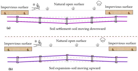
Figure 4.
Pipe movement in the vertical direction is attributed to seasonal moisture changes in expansive soils: (a) dry season; (b) wet season.
Individual wooden poles used for overhead electrical and telecommunication distribution networks can also be vulnerable to soil movement as a result of improper foundation design and insufficient site investigations before installation [48]. Likewise, differential movement between a manhole cover and surrounding expansive soils can be seen in Figure 5, and the performance of an underground structure can also be affected by crack propagation and the associated stress.
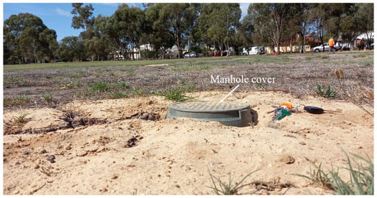
Figure 5.
Surface cracks on the ground surface and settlement due to soil shrinkage around a manhole cover during dry season.
The presence of shrinkage cracks also has a significant role in slope instability, where repeated shrink–swell cycling can lead to progressive failure and create an easier path for rainfall to reach the shear surface, as shown in Figure 6. Therefore, the shear surface experiences increased pore water pressure during rainfall events, which can lead to slope failure [49]. This was also reported by Chao et al. [50], who noted that the reduction in soil strength due to the decrease in matric suction resulting from the shrinkage crack-induced infiltration triggered the instability of a reactive soil embankment. Furthermore, cut slopes can deteriorate through the dissipation of pore water pressure (PWP) induced by excavation or the seasonal cycling of PWP [51]. An accelerated progressive failure of the slope owing to the reduction in strength can be expected to occur with dry and wet cycles having greater magnitudes and frequencies [12].
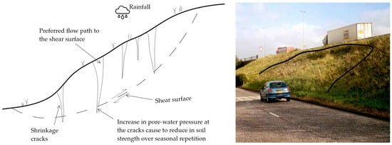
Figure 6.
Triggering of slope instability in clay soil prone to shrinkage.
4. Investigations of Expansive Soil Behaviour
Several laboratory, field, and numerical studies have investigated different aspects of the soil–atmospheric boundary interaction for expansive soils. A summary of the observations of these studies is presented in this section.
4.1. Laboratory Investigations
In unsaturated soils, the soil desiccation state can be better understood based on the soil suction, which represents the affinity of soil toward the water. Soil movement is directly related to soil suction; the higher the suction, the higher the potential for soil movement will be. Various techniques can be applied to measure the suction, such as filter paper (in contact and non-contact), pressure plates, and relative humidity methods, including the electrical conductivity (EC) method. For example, Agus et al. [52] performed measurements on filter paper discs (Whatman No. 42) and developed Equations (1) and (2) to describe the relationship between the suction (metric suction, um, and total suction, ut) and the water content of the filter paper (wfp) based on best-fit regressions. To determine the solute suction (us) using the EC method, Equation (3) can be used. Equation (3) incorporates the actual moisture content (amc) to represent field conditions in which soil and water at a ratio of 1:5 are used to estimate the salinity of the soil–water suspension in the laboratory.
Changing climatic conditions alter the moisture content of soils. This will affect not only the suction but also the permeability of the soil. The relationships between the soil suction, moisture content, and permeability can be expressed as the soil–water characteristics curve (SWCC) and the hydraulic conductivity function [53], which are important parameters for understanding expansive soil behaviour. The SWCC can be generated using various methods. One of these is to utilise the water content and suction values measured in the field or laboratory. These data can then be used to fit the functions available in the literature [54,55]. For instance, Equation (4), proposed by Van Genuchten [54], can be used to deduce the SWCC.
where θ is the volumetric moisture content; θr is the residual volumetric moisture content; θs is the saturated volumetric moisture content; ψ is the soil suction; and a, n, and m are empirical fitting parameters related to the SWCC, with .
Another method for estimating the SWCC is to use empirical correlations based on basic soil parameters (grain size distribution, liquid limit, void ratio, etc.) [12,56]. Several methods are available [57,58,59,60,61] for predicting the SWCC based on the directly measured geotechnical parameters of a specific soil. Depending on the availability of site-specific soil data, an appropriate function can be used. For instance, based on the saturated moisture content (ws), plasticity index (PI), and fine content, Witczak et al. [61] proposed Equations (5)–(10) to estimate the SWCC relating θ and the soil suction (in kPa).
Here, the weighted plasticity (wPI) is obtained by multiplying PI and the percentage of clay in the soil. Witczak et al. [61] further described the constraints applied in the above equations as follows:
ws can be estimated using Equation (12) [62].
af = 5 for af < 5 and cf = 0.03 for cf < 0.01
Karim et al. [12] compared the SWCCs developed using the above methods, including SWCCs predicted for similar soils, as shown in Figure 7, to observe the PWP changes in an infrastructure slope induced by meteorological changes. However, these methods may not be very accurate unless they are supported by extensive field investigations. A better agreement among the results was obtained from the analysis using an SWCC acquired from field data than that using an SWCC obtained from a weighted PI and a similar soil (London clay) for the measured values of the positive PWP, θ, and soil suction variation with the depth.
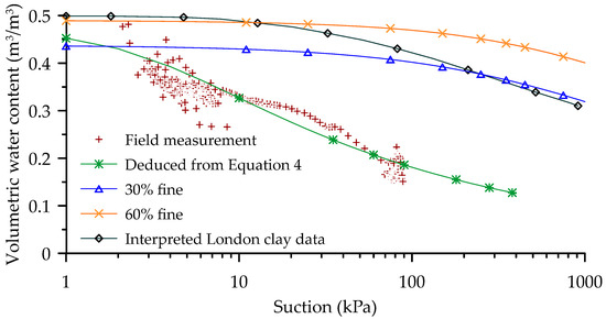
Figure 7.
SWCCs used for analysis of a cutting in weathered London clay in Newbury, England. Field data and interpreted London clay data taken from Karim et al. [12], 30% and 60% fines data are generated by fitting Witczak et al. [61] equations.
Aubertin et al. [57] developed a modified Kovács [63] (MK) model for the prediction of SWCCs for various soil types (tailing materials, cohesive and cohesionless soils) assuming two mechanisms of soil moisture, namely capillary saturation (Sc)–capillary force-associated saturation and adhesive saturation (Sa)–adhesive force-associated saturation, as shown in Equation (13) (mathematically rearranged by Fredlund et al. [64], Bussière [65]). The proposed MK model comprises Equations (13)–(23) to estimate the SWCC relating Sa and Sc. This model requires basic soil properties, i.e., grain size distribution and liquid limit.
where S is the degree of saturation, θ is the volumetric moisture content, n is the soil porosity, and are Macauley brackets . Here, y is an open variable.
The empirical relationship between Sc and suction is represented by Equation (14).
where hco is the equivalent capillary rise (cm), ψ is the soil suction (cm), and m is a unitless pore size distribution parameter.
The empirical relationship between Sa and the suction is represented by Equation (15).
where ac is the dimensionless adhesion coefficient, e is the void ratio, is the suction of the soil under completely dry conditions (cm) ( cm of water, which approximately corresponds to S = 0), ψn is a normalisation parameter for maintaining unit consistencies (equal to 1 cm if the ψ values are in cm), and is the residual suction (cm).
For the computation of the MK model, the required parameters are hco, m, , and ac. For granular soil, these parameters are expressed as follows:
where D10 is the particle size corresponding to the tenth percentile of the particle size distribution curve, and is the uniformity coefficient, which is equal to . Here, D60 is the particle size corresponding to the sixtieth percentile of the particle size distribution curve.
For plastic–cohesive soil, these four parameters are expressed as follows:
where is the density of solid particles (kg/m3), and is the liquid limit (%).
The hydraulic conductivity (K) of soil describes the rate of moisture movement through the soil. The value of K for saturated soil (Ksat) can be determined through various permeability tests, such as falling head or constant head tests. However, the measurement of K for unsaturated conditions (Kunsat) is difficult in laboratory or field tests as Kunsat is dependent on the soil suction. The hydraulic conductivity function can be estimated using correlations proposed in various studies [54,66,67], which generally take the soil suction and Ksat as input parameters, as shown in Equation (24), proposed by Van Genuchten [54]. Using this equation, Kunsat can be estimated through a back-analysis of the field data as a function of Ksat, as demonstrated by Karim et al. [15].
where ψ is the soil suction, and a′, n, and m are empirical fitting parameters.
The behaviour of expansive soil is strongly influenced by the drying environment and the number of wetting and drying cycles. Kong et al. [68] conducted a series of shrinkage tests under different drying temperatures and relative humidities, as well as triaxial tests on undisturbed samples prepared under different drying conditions. They observed that a reduction in temperature and an increase in relative humidity reduced the drying rate. Moreover, the drying rate could be used to characterise the soil. Furthermore, they reported that the drying rate was inversely correlated with linear shrinkage and soil strength.
Zhan et al. [69] investigated the softening characteristics resulting from the wetting state of soil using suction control triaxial tests on recompacted and undisturbed samples. A considerable part of the plastic strain arose from the wetting-induced swelling of the soil, and this strain decreased with an increase in confining pressure.
Linear shrinkage tests are commonly performed on expansive soils. Puppala et al. [70] noted that these tests have various limitations, including a smaller sample size, lateral restriction of the soil due to the rigidity of the moulds, and manual errors in measurement. To overcome these limitations, a new methodology for conducting volumetric shrinkage strain experiments on cylindrical soil samples was proposed, including a digital imaging procedure through which volumetric shrinkage strains could be determined.
The swelling behaviour of expansive soils can be observed through volumetric free swell tests, in which swelling movements in the radial and vertical directions are measured by a dial gauge and Pi tape, respectively, at several periods. Puppala et al. [71] developed correlations between the shrink–swell displacements, the plasticity of soil, and several compaction properties related to seasonal moisture alterations in an underlying soil. The proposed correlations could be used for the prediction of vertical soil movements.
4.2. Field Investigations
Although field investigations can reflect actual soil behaviour, such as crack formation and propagation, soil movement, and moisture migration within the soil, these studies are limited by their high time and cost requirements [72]. One well-instrumented site study was performed by Fityus et al. [73], who conducted a long-term field study near Newcastle, Australia. Their study obtained high-quality data focusing on variations in the soil moisture content and suction, including ground movements at depths of up to 3 m. In addition, covered and uncovered hydraulic boundary conditions were established by providing two ground covers (flexible and reinforced concrete) and maintaining open space, respectively; the effect of trees was also investigated. The results revealed that the soil tended to present a heaved condition. This could be expected, as the estimated Thornthwaite moisture index (TMI) was +25 [74], suggesting a surplus condition of long-term moisture. Furthermore, the active soil depth and soil suction change were estimated to be 1.6–1.7 m and 2 pF, respectively, suggesting that the depth of suction change and surface suction change given in AS2870 [75] require some improvements to capture the particular site condition. In addition, their observations indicated that the presence of trees could increase the active depth. Moreover, the outcomes with the flexible cover indicated that the centre-heave mound may be critical during dry periods in a long-term scenario. The centre-heave mound resulting from a surface covered in reinforced concrete presented an unusual compound mound shape having dish features inside the edge beams, suggesting a significant influence of these beams for preventing horizontal moisture movement from the boundaries of the cover.
Li and Guo [76] conducted a site study on a residential building in Melbourne, Australia affected by reactive soil movement attributed to tree root drying; the building was constructed on highly reactive soil. Some defects were observed, such as tilting of the building floor, differential displacement (maximum of 125 mm) between two corners, and cracks on the walls. Their investigation of the soil suction revealed that the moisture content up to a depth of nearly 3.5 m was influenced by the presence of large trees (eucalyptus). This indicates the significance of proper site management for lightweight buildings on reactive soils, as trees growing close to a house can result in more damage than the anticipated moisture variations, owing to the seasonal changes and redistribution of moisture patterns from the presence of infrastructure.
Cheng et al. [77] performed a field test in Kenya over a period of 14 months using square footings (2 m × 2 m) instrumented with probes to measure the moisture content. In addition, a digital level was used to record the monthly vertical movement of the foundation, and buried water content probes were deployed to monitor the moisture movement within the soil. They found significant variations in the moisture content with the depth and season as shown in Figure 8 (estimated volumetric water content data from an uncovered site in South Australia is also added to the figure); a greater variation in the moisture content was observed near the surface which reduced with depth. In addition, an increase in the settlement and heave of the foundation was recorded in dry and rainy seasons, with 45 and 28 mm of settlement and heave, respectively, as maximum values at the top surface of one foundation; similar values of 47 and 26 mm, respectively, were observed for another foundation.
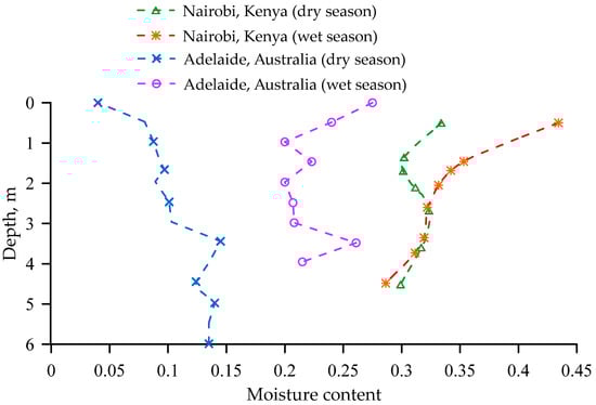
Figure 8.
Average measured soil moisture content variation with depth below the foundation in Nairobi—selected datapoints from Cheng et al. [77] with the permission of Taylor and Francis Ltd., and below an open field in Adelaide—estimated water content from suction measurement by Mitchell [78].
Karunarathne [56] conducted a field study to monitor the soil profile at a study site in Melbourne. Based on their findings, significant ground movement was not expected below a depth of 1.25 m as no considerable soil moisture changes were observed below this depth. Furthermore, it was found that the monthly rainfall correlated well with the soil movement (Figure 9) in the upper layers, with a specific time lag related to the soil permeability. The swelling and shrinking of soil in winter and summer, respectively, followed the rainfall trends, and the sensitivity of the soil movement to precipitation decreased with increasing depth (Figure 9).
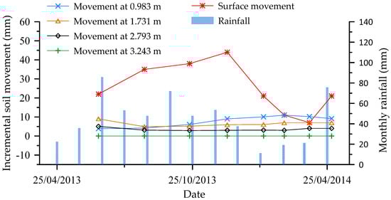
Figure 9.
Soil movement associated with monthly rainfall. Data from Karunarathne [56].
Fernandes et al. [79] used several sensors for the continuous measurement of the movement of a clay layer along with variations in the temperature and moisture content of the soil. Correlations between these parameters and the annual climatic changes observed at site-specific meteorological stations were then developed. They found significant changes in the temperature and moisture content up to a depth of 3 m. Their study improved the understanding of the medium-term shrink–swell behaviour of clay soils, as the study encompassed five drought–rewetting cycles.
These field studies indicate that climate variations (seasonal, medium-term, and long-term) can have a significant impact on infrastructure through the moisture-induced shrink–swell behaviour of soils. For cases where field data are not available, results from field observations at other sites can be extrapolated to obtain a preliminary estimation of the soil behaviour based on the suitability of the climate. In addition, numerical analyses can be performed using the data from field case studies for model validation, which can improve confidence in the performance of the numerical model and the ability of the model to produce realistic predictions.
4.3. Numerical Investigations
Many studies have been conducted to understand the effects of weather parameters such as rainfall and temperature on soil moisture changes; the effects of these parameters on the suction change and shear strength of the soil have also been explored using various analytical tools in different climatic conditions [12,17,28,80,81,82,83]. For instance, Toll et al. [84] developed an unsaturated flow model in Seep/W using permeability and water retention data to observe the field-level pore water pressure variation resulting from rainfall events. Then, a hydromechanical model was developed using Plaxis software to evaluate the mobilised shear strength of the slope based on the change in the pore water pressure and the factor of safety over time resulting from actual rainfall. It was found that the decrease in shear strength was more rapid during a rainfall event than its recovery during drying, which indicated a rapid reduction in shear strength during recurring rainfall events with shorter drying periods. Here, an anisotropic condition of the permeability was expected owing to cracks, and the model outcome could be improved by including this parameter.
The movement of expansive soils results in another cluster of problems related to the serviceability of infrastructure. To obtain a better understanding of the interaction between expansive soils and structures in response to moisture variations, limited studies have been conducted on the footing design [85,86,87], canals [88], pipelines [47,89,90,91], slopes [50], pavements [92], etc. In most of these studies, atmospheric conditions were obtained from field investigations in which changing climatic conditions were overlooked. Thus, although climate change is likely a driver of the worsening of infrastructure problems, limited attention has been paid to soil moisture–structure interactions focusing on lightweight infrastructure. In this context, Karunarathne et al. [93] aimed to incorporate long-term climatic scenarios in the analysis of ground movement. Similarly, Teodosio et al. [85] conducted a recent study on soil–structure interactions combining most of the possible mechanisms involved in expansive soils. Hence, it is worthwhile to discuss these two studies to understand expansive soil behaviour in the Australian climate.
Karunarathne et al. [93] developed a Vadose/w model to observe the water content variation of an expansive soil based on seasonal climatic variations; the model was validated through regular field monitoring. For the Vadose model, hydraulic properties including the SWCC were obtained from soil investigations (laboratory and field), whereas, for the thermal properties, data from nearby sites were used. The other input parameters are presented in Appendix A, Table A1. Figure 10 compares the measured and predicted moisture content; the results demonstrate that the model can reliably predict moisture changes in all seasons. A slight deviation is observed near the surface. This is expected because of the local influences on the surface owing to the existence of slope variations, potholes, shrinkage cracks, and differences in vegetation.
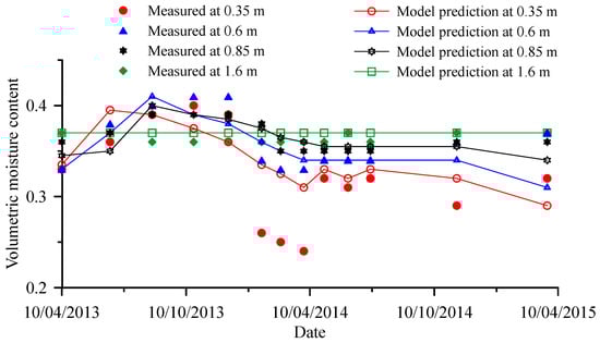
Figure 10.
Measured and predicted soil moisture at various depths. Data from Karunarathne [56].
The probable ground movements were then estimated using FLAC3D based on the outcomes of the Vadose/w model, assuming isotropic free swelling of the soil, and the results were validated based on site measurements of the ground movement. The input parameters and equations used in the simulation are listed in Appendix A Table A2 and Table A3, respectively. This model can be used to predict ground movement under long-term climatic conditions. However, further studies can improve the functionality of the model based on spatial variations to capture local conditions. For instance, if the model was generated by considering different regions of Australia for different representative concentration pathways, it could provide better predictions than the model generated by averaging the projected rainfall and temperatures of different cities.
Teodosio et al. [85] developed a hydromechanical model using Abaqus software to evaluate the combined interaction of the soil moisture variation in expansive soil and changes in loading conditions on structures. To model the soil moisture variation, SWCC data reported by Li et al. [94] for the same site were used. To describe the mechanical behaviour of the soil, the Bishop [95] function was simplified as shown in Equation (25); to describe the soil–structure interaction, contact element analysis [96] was used. Appendix A Table A1, Table A2 and Table A3 list the input parameters and equations used in these studies.
where σ is the total stress resulting from the mechanical load, is the effective stress, ψw is the soil suction, and Sr is the degree of saturation. The incremental stress (dσ′) can be expressed as shown in Equation (26) [97].
where E is the elastic constant tensor of the soil, κ is the logarithmic bulk modulus of the soil, eo is the initial void ratio, is the volumetric strain obtained through laboratory shrinkage experiments, and and are the initial and final equivalent stress components, respectively, of the orthogonal stresses.
The simulated outcomes are compared to field observations (average of upper and lower bound observations) in Figure 11. The field data (gravimetric soil moisture, soil suction, and reactive soil movement) was collected by Fityus et al. [73] over a five-year period. It can be seen that for both edge and centre heave, reasonable prediction of ground movement is achievable even though there are significant scope for improvement of accuracy. There is a need for further studies to better understand the interaction between structures and underlying reactive soils. It is expected that simulations can overcome most of the shortcomings associated with uncoupled traditional methods, preventing oversimplification by considering the 3D moisture flow and associated mechanical behaviour to represent a more realistic soil movement profile. Incorporation of effect of vegetation and effect of climate change in such analyses can be of interest to the general engineering community.
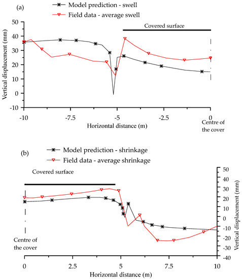
Figure 11.
Comparison of simulation results against field measurements; simulation data from Teodosio et al. [85] and field measurement data from Fityus et al. [73] for the (a) edge heave; (b)centre heave.
The ground movement associated with climate change can increase the susceptibility of growing urban areas to damage; however, recent urban development planning strategies have not considered the impact of climate change on housing foundations in Australia [98]. In this scenario, it is vital to investigate the behaviour of expansive soils for infrastructure resistance to climate change, and two studies [85,93] conducted in Melbourne can provide a better understanding of soil–atmosphere–structure interactions. As the climates of other states in Australia are different, it is essential to conduct such studies in other regions as well. If these studies are compared, the former can incorporate long-term climate conditions to estimate ground movement in response to future climate, whereas, in the second study, the inclusion of future climatic conditions has not been considered. Hence, an improved model can be developed using the concept of volumetric strain and incorporating future climate conditions.
5. Australian Design Practice for Residential Footings on Expansive Soils
More than 30% of Australian surface soils, distributed as shown in Figure 12, can be classified as expansive [16]; they can also be found in all inhabited continents of the world [44]. The Australian standard for footing design for residential buildings, AS2870 [75], classifies sites according to the characteristic surface movement (ys). Here, ys is defined as the movement of the ground in the vertical direction owing to long-term suction changes in the soil. The site classes ranges from mostly sandy and rocky non-reactive sites (ys = 0 mm) to extremely reactive sites (ys > 75 mm). ys is also used in the design of other structures on expansive soils, such as road pavements [99,100].
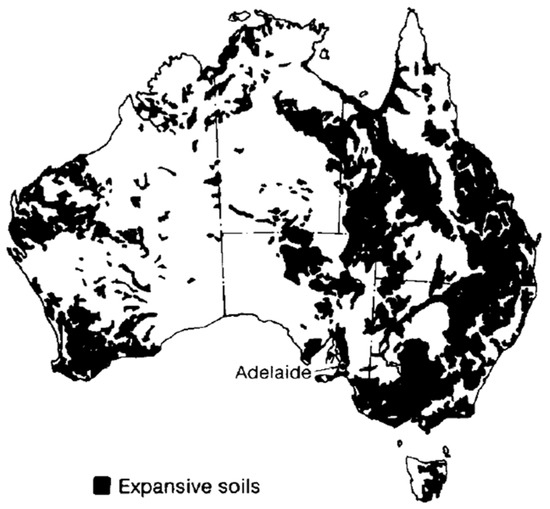
Figure 12.
Distribution of expansive soils in Australia. Source: [101].
5.1. Characteristic Surface Movement Prediction
The characteristic surface movement, ys, can be calculated as the cumulative movement of the individual sublayers of soil within the design suction change depth (Hs), as shown in Equation (27) [75].
where Ipt is the instability index (%/pF), is the average soil suction change of a particular layer (pF), h is the thickness of a particular layer (m), and N is the number of soil layers within Hs.
5.1.1. Instability Index
AS2870 [75] defines the instability index (I) as shown in Equation (28).
where ε is the vertical strain, and Δu is the suction change. I can be deduced from a core shrinkage test [102], loaded shrinkage test [103], and a combination of shrinkage and swelling tests [104]. I can also be estimated from a visual–tactile investigation, and some correlations between I and other index tests for clay exist, e.g., the linear shrinkage test. I obtained from the shrink–swell test is referred to as the shrink–swell index (Iss) and can be estimated using Equation (29) [104].
where is the swelling strain (%), which is zero for < 0, and is the shrinkage strain corresponding to the oven-drying condition (%).
I obtained from the loaded shrinkage test is defined as the loaded shrinkage index (Ils) and can be estimated using Equation (30) [103].
where c is the soil moisture characteristics defined as in Equation (31), and S is the slope of the strain versus moisture content plot defined as in Equation (32).
where wo is the water content of the sample trimmings, wf is the final water content of soil (%), uo is the mean soil suction of the sample trimmings, and uf is the mean soil suction determined from the sub-samples acquired after the sample’s removal from the apparatus (pF).
where is the change in sample strain (%), is the change in the water content (%).
The index obtained from the core shrinkage test is defined as the core shrinkage index (Ics) and can be estimated using Equation (33) [102,105].
where Δε is the shrinkage strain (%), Δwc is the variation in the moisture content (%), and c is the soil moisture characteristics, defined as below:
where wc is the water content of a soil disc (%) at the mass equilibrium point when the specimen is kept in a chamber with supersaturated ammonium chloride solution, wo is the initial water content of the sample trimmings, and uo is the initial total suction (pF).
In core shrinkage tests, the occurrence of shrinkage cracks may lead to inaccurate lengths, and difficulty in determining the moisture characteristics may lead to deviations in the results. There is also the possibility of a loss of soil crumbs during handling, and, hence, these tests may not be the preferred method for estimating soil reactivity [106]. The calculation of Iss involves both swelling and core shrinkage tests; however, controlling the suction can be difficult, and lateral confinement of the sample during the swelling test allows only vertical movement to occur. In addition, neglecting the solute suction expected from mineralised soil by using distilled water may affect the accuracy of the results. Despite the limitations of Iss, it captures the shrink–swell properties, and thus it can be considered a more reliable reactivity index than Ics. This observation was supported by Fityus et al. [107] and Cameron [108]. Furthermore, the shrink–swell test method does not require tests for suction and can be applied to any given initial moisture condition of the soil [109].
The laboratory test conditions (e.g., one-dimensional swelling in swelling test and unrestrained shrinkage in core shrinkage test) can often vary from the field condition. In the field, cracks are often present up to a certain depth and the confinement and overburden pressure change with the soil depth (z). To correct for the field effect, a multiplier, the lateral resistance factor (α), is applied to the lab-deduced reactivity index (Ips), as shown in Equation (35) [75]. Please note that Ips is used here as a generic reactivity term, and, depending on the method used, Ips can be Ils or Ics or Iss.
Ipt can be defined as the field reactivity index after adjustment of the laboratory-deduced index for field conditions. In the cracked zone, lateral confinement is not expected, and α can assume a value of 1 [107]. To account for the lateral confinement beneath the cracked portion, the relationship presented in Equation (36) has been used [75]. Here, α is again assumed to be equal to 1 for depths of greater than 5 m to achieve a value of Ipt that is at least equal to Ips.
Once the value of Ipt is determined, soil can be classified as of low, moderate, high, and very high expansive nature, as shown in Table 2 below. It is to be noted that other index properties (liquid limit and plasticity index) have also been used for deducing the soil’s classification, and this is also presented in Table 2. Others have correlated the reactivity with linear shrinkage strain, even though the correlation can have low reliability [110].
Table 2.
Guide for expansive soils classification [99,111,112,113].
5.1.2. Depth of the Design Soil Suction Change (Hs)
Hs is the soil depth under which the soil moisture content is not affected by seasonal climate variations; hence, no suction changes occur, and soil below this depth does not contribute to ground movement. The location of the water table and bedrock affects Hs [75]. In such situations, adjustments to Hs and the suction profile can be made, as shown in Figure 13. For example, when a shallow depth water table is present, the suction triangle should end at the top of the water table. In presence of bedrock, the triangle reaches to the full depth of suction change but the calculation from rock layer is ignored.
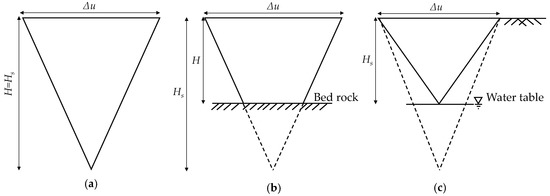
Figure 13.
Suction profile simplifications under various scenarios (a) soil to depth ≥ Hs; (b) effect of bedrock; (c) effect of groundwater. Adapted from [75] by the first author with the permission of Standards Australia Limited under licence CLF1022BD. Copyright in AS 2870-2011 vests in Standards Australia. Users must not copy or reuse this work without the permission of Standards Australia.
5.1.3. Soil Suction Change at the Ground Surface (Δu)
Suction is a function of the moisture content and soil type and it varies in response to atmospheric boundary interactions. AS2870 [75] provides a constant Δu value (1.2 pF) for various locations in Australia. Suction can be measured through field monitoring at various depths in different locations according to the season. AS2870 [75] assumes a triangular variation in the suction profile as shown in Figure 13a. However, this triangular distribution of Δu is usually assumed to be conservative because the variation is not linear with depth; rather, it declines more rapidly, as shown in Figure 14, and thus underestimation may be expected near the surface [114].
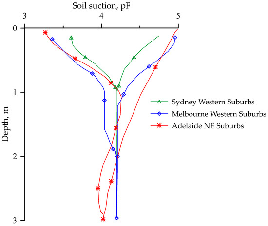
Figure 14.
Field observations of suction changes for extremely dry and wet conditions. Data adapted from [114] by first author with the permission of Standards Australia Limited under licence CLF1022BD. Copyright in HB 28-1997 vests in Standards Australia. Users must not copy or reuse this work without the permission of Standards Australia.
5.1.4. Mound Shape and Soil’s Stiffness
The shape of swelled or shrunk ground is referred to as the mound shape, and different formulations have been published in the literature to capture this. For instance, AS2870 [75] includes two recommended methods, namely the Walsh [115] and Mitchell [116] methods. In Walsh’s method, the edge distance (e) and differential mound movement (ym) across a foundation are used to define the mound shape, with flat mounds having parabolic edges, as shown in Figure 15, where ym can be considered as 0.5ys and 0.7ys for the edge heave and centre heave, respectively [75]. Likewise, different values of edge distances (m) are given for edge heave and centre heave, as shown in respective Equations (37) and (38).
where L is the length of the slab in m and ym is in mm.
where ym is in mm and Hs is in m.
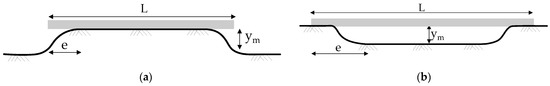
Figure 15.
The idealisation of mound shapes in Walsh’s method to depict ground movement in design: (a) centre heave; (b) edge heave.
The idealised mound shape in Mitchell’s method can be presented as shown in Figure 16, where ym can be considered as 0.7ys for both conditions (edge heave and centre heave) [75]. The profile of the mound in the x and y axes can be obtained from the following Equation (39).
where c is calculated from the deflected boundary condition at the centre of the slab and m is the mound exponent given by Equation (40).
where ym is in mm, Hs is in metres, and De is the embedment depth of the edge beam in metres.
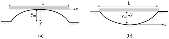
Figure 16.
The idealisation of mound shapes in Mitchell’s method to depict ground movement in design: (a) centre heave; (b) edge heave.
The design tree effect as a surface movement yt can be calculated using the equation below [75]:
where HT is the height of a single tree, Dt is the distance of the tree from the building, Di is the influence distance. For a single tree, Di should be taken equal to HT of a group of 4 or more trees in a row; Di can be taken as twice the design height of the tree group. yt-max is the maximum potential surface movement induced by tree-related suction change. This is in addition to the usual design suction profile suggested by the design code. A similar method as of ys for a regular site can be used to calculate yt-max. The depth of cracking can be taken equal to the maximum design drying depth.
AS2870 [75] suggests the ranges of mound stiffness for swelling and shrinking or stable soils. For beams in interaction with swelling soil, the value of soil stiffness (k) ranges between 400 kPa/m and 1500 kPa/m, which may be used as below [75].
where q is the ratio of total building load to the plan area of a slab and k should be at least 1000 kPa/m. For beams in interaction with stable or shrinking soil, k should not be less than 5000 kPa. Besides these values mentioned in the Australian Standard, some other approximations have been made, such as bi-linear [115] and non-linear [116] relationships between swelling and applied pressure.
5.2. Effect of Climate on Hs and Correlation with TMI
The regional climate has a specific relationship with Hs. A reliable value of Hs can be achieved based on long-term site data of ground movements and suction changes, including moisture variations with depth. However, obtaining these data requires not only an extensive site investigation program but also a longer period of up to decades for data acquisition and accumulation [117]. Few investigations have been performed to predict Hs for various locations in Australia. For example, Hu et al. [118] estimated Hs values for three locations in Western Australia and compared them with the available site data [119], while Walsh et al. [117] developed Hs maps for south Western Australia and South-Eastern Queensland, and Fityus et al. [74] generated a Hs map of the Hunter Valley region of New South Wales, with a discussion of the Hs values at three locations within the Hunter Valley region. With limited field observations, AS2870 [75] presents values of Hs for specific locations, where higher values of Hs correspond to hotter climate zones; this can be extrapolated to other areas based on the suitability of the climate. Alternatively, the TMI is a widely accepted moisture index for incorporating the effect of climatic boundary conditions in geo-infrastructure design; hence, AS2870 [75] provides relationships between Hs and TMI values (Table 3) so that Hs can be estimated based on the TMI of a particular site. One limitation of AS2870 was that it provides the Hs recommendation for ranges of TMI values which may create confusion in certain cases. Fityus et al. [74] presented a continuous relationships between Hs and TMI. It is expected that climate change will cause changes in TMI, which will influence Hs which can be an important problem requiring future investigation.
Table 3.
Relationship between TMI and Hs. Adapted by first author with the permission of Standards Australia Limited under licence CLF1022BD from [75]. Copyright in AS 2870-2011 vests in Standards Australia. Users must not copy or reuse this work without the permission of Standards Australia.
5.3. Comparison with American Practice on Expressing Expansion Potential
In the USA, with the evaluation of various published criteria to classify the expansion potential, Snethen et al. [120] argued that the liquid limit and plasticity index can be taken as the best indicators for predicting soil’s potential to expand, as shown in Table 4 The environmental conditions can be represented by this approach, as it considers the field soil suction as well. This approach has been adopted by AASHTO for classifying the expansion potential of soil [121], whereas characteristic surface movement is used to characterise the site in Australian practice. Lytton et al. [122] and Zornberg et al. [123] presented the methods for estimating vertical strain from volumetric strain exerted by expansive soil along with the soil suction profile prediction for the transient states. Their studies have concentrated mostly on pavement design on expansive soil. For the residential footing design, among various methods, the Post Tension Institute (PTI) method is well employed in the USA, which has some similarity with AS2870 [75], such as the consideration of edge heave (lift and drop) depending on the distance of the edge, moisture change, and the expected differential movement from the shrink–swell phenomenon as per climate conditions [124].
Table 4.
Expansion potential of soil. Adapted from Snethen et al. [120].
5.4. Summary
AS2870 [75] provides a simplified method for estimating the characteristic surface movement (ys) and classifies sites according to their characteristic ground movement, e.g., sandy and rocky sites (class A) to extremely reactive clay sites (class E). A subscript D is added to the classification if the depth of suction change is >3 m. The current standard provides the basic requirements for the design of slabs and footing for residential buildings, emphasising expansive soil issues. It also provides guidelines on the estimation of the depth of suction change based on TMI. However, the available TMI maps may not reflect the current climate [98]. Furthermore, the suction depth to TMI relationship has been developed based on limited field investigations [76]. It is also believed that the change in suction assumed at the ground surface (used in ground movement calculation) is a function of soil type and climate conditions. AS2870 [75] provides very limited guidance on its value.
With an example of a specific site in Melbourne, Mitchell [125] mentioned the continuing revision requirement for the design standards to incorporate the climate change effects. These indicate the importance of incorporating the effect of the changing climate to ensure safer, more economic, and climate-resilient designs. Karim et al. [16] showed that the changes in TMI and thus suction depth may not be uniform across all sites, with dryer areas being less affected compared to wetter areas within the state of South Australia. This indicates a necessity of taking site-specific TMI calculations to capture future changes. The effect of the climate inputs can also be accounted for in more sophisticated numerical simulations. However, this can be a complex process and research is underway to better understand the interaction between the expansive soils and the atmospheric boundary. Hence, by varying these climatic inputs, various numerical simulations can be performed to represent various locations to either better understand the process or to design for the specific site boundary condition and soil type.
6. Conclusions
Expansive soils are problematic soils. They change volume and can exert additional stresses founded on or within shallow depths. Relevant literature has been reviewed in this paper and the important outcomes are summarised here.
- The behaviour of expansive soil can be complex. The expansive soil movement can be influenced by several factors, including its mineralogy and hydraulic and atmospheric boundary condition.
- Many different types of structures can be affected. Some of the specific examples found in the literature are lightweight residential buildings, road pavements, underground pipelines, slopes, and other infrastructures.
- It is expected that, due to climate change, the problems due to expansive soils will worsen in many parts of the world and should be given proper consideration for building climate-resilient structures.
- The effect of climate change may not be uniform across a state or other jurisdiction, and the local condition needs to be taken into account (calculation of local TMI and other variables may be needed).
- Laboratory tests commonly used for the quantification of reactivity are simplified and can be time-consuming. The number of field studies is also limited due to the expenses and effort involved.
- Current practice is based on a simplification of a complex process and caution should be exercised when estimating the soil reactivity as a function of conventional soil parameters such as the liquid limit or plasticity index.
- Numerical tools have been used to capture the behaviour of expansive soil and its interactions with different types of structures and can be a useful tool for a better understanding of the process or site-specific designs. They can be categorised into three groups, i.e., (1) modelling of the seepage due to interaction with the atmospheric boundary; (2) modelling of volume change and related ground movement, and (3) modelling of the interaction between the soil and structure constructed on or within the shallow depth of it.
- Advanced numerical methods for unsaturated seepage will require inputs of the SWCC and unsaturated hydraulic conductivity function and can be a complex process.
- Several past studies have attempted modelling of the interaction between soil–atmospheric boundaries and structures. However, several assumptions have been made, including some on the calculation of effective stress, which can have important consequences for the outputs of the numerical model.
- This review recommends further studies to incorporate the effects of the future climate, as geo-structures are designed to achieve a 50- to 100-year service life.
Author Contributions
Conceptualisation, B.D. and M.R.K.; methodology, B.D. and M.R.K.; formal analysis, B.D.; investigation, B.D. and M.R.K.; resources, M.R.K., M.M.R. and H.B.K.N.; data curation, B.D., M.R.K. and H.B.K.N.; writing—original draft preparation, B.D.; writing—review and editing, M.R.K., M.M.R. and H.B.K.N.; visualisation, B.D. and M.R.K.; supervision, M.R.K., M.M.R. and H.B.K.N.; project administration, M.R.K. and M.M.R. All authors have read and agreed to the published version of the manuscript.
Funding
This study received no external funding. However, the first author of this paper was supported by President’s Scholarships from the University of South Australia towards his Ph.D. study.
Institutional Review Board Statement
Not applicable.
Informed Consent Statement
Not applicable.
Conflicts of Interest
The authors declare no conflict of interest.
Appendix A
Table A1, Table A2 and Table A3 list the parameters and equations used in the numerical simulations.
Table A1.
Parameters used to model the soil moisture variation.
Table A1.
Parameters used to model the soil moisture variation.
| SWCC | Hydraulic Conductivity Function | Thermal Properties | Climate Data | Vegetation Influence | Boundary Condition | Reference |
|---|---|---|---|---|---|---|
| Developed through the measured soil suction with corresponding moisture content in Vadose/w software | The equation proposed by Fredlund et al. [67] was used to develop this function in the Vadose/w model. Ksat was measured. | The measured thermal conductivity, including the specific heat capacity variation with the moisture content, was taken from another site near the study area [126]. | Weather data collected from the nearest weather station were assigned in the Vadose/w model. | Considered in Vadose/w through LAI, RD, and PML factors. |
| [93] |
| Obtained from Li et al. [94] | Kunsat was formulated based on Forchheimer [127]. Ksat = 1 × 10⁻⁷ to 1 × 10⁻⁹ (m/s). | - | - | - | A soil column of height:width:length = 11:11:11 m was considered to avoid the impact of boundary conditions. | [85] |
Here, LAI is the leaf area index, RD is the root depth, and PML is plant moisture limiting.
Table A2.
Parameters used for the soil suction and volume change/deformation analysis.
Table A2.
Parameters used for the soil suction and volume change/deformation analysis.
| Suction Change | Hs(m) | Strain | Reference |
|---|---|---|---|
| SWCC from Vadose/w model captures the suction profile | 0.6 to 3 | , α = 0.28 [128] | [93] |
| 1.2 pF | 1.3 to 4 | [85] |
Here, Δεsh is the linear swelling strain, Δw is the change in water content, α is the linear expansion coefficient, is the total strain, is the strain resulting from the effective stress of the soil, and the volumetric strain resulting from the swelling of soil based on the moisture level.
Table A3.
Determination of the stress in soil based on the moisture-induced strain.
Table A3.
Determination of the stress in soil based on the moisture-induced strain.
| Stress Equation | Bulk Modulus | Elastic or Shear Modulus | Poisson’s Ratio | Boundary Condition | Reference | |
|---|---|---|---|---|---|---|
[128] | Second-order polynomial equation in the FLAC3D model was developed from lab tests of the soil to generate the soil stiffness (E) and gravimetric moisture relationship. | νsoil = 0.45 | Same as Table A1. | [93] | ||
| Equation (25) Equation (26) | Log bulk modulus, κ, commonly adopted values were 0.01–0.06. | E = tensor of soil elastic constants | νsoil = 0.1 to 0.4 |
| Mechanical behaviour of soil | [85] |
| Elastic modulus of concrete (Ec) = 20–25 GPa | νconcrete = 0.2 | Slab-on-grade model | ||||
Here, is the stress change, k is the tangent bulk modulus, ν is the Poisson’s ratio, is the change in deviatoric stress, is the change in the elastic part of the deviatoric strain, is the elastic volume change (logarithmic), G is the shear modulus, eo is the initial void ratio, is the uniaxial tensile stress, is the uniaxial compressive stress, dt and dc are damage variables ranging from zero (undamaged concrete) to one (damaged concrete), and and are the tensile and compressive plastic strain rates, respectively.
References
- Hasan, S.; Patowary, M.Z.; Sazzad, M. Comparison of the behaviour of expansive soil using different admixtures. In Proceedings of the Second International Conference on Research and Innovation in Civil Engineering, Chattogram, Bangladesh, 10–11 January 2020. [Google Scholar]
- Koukouzas, N.; Tyrologou, P.; Koutsovitis, P.; Karapanos, D.; Karkalis, C. Soil stabilization. In Handbook of Fly Ash; Elsevier Inc.: Amsterdam, The Netherlands, 2022; pp. 475–500. [Google Scholar]
- Nelson, J.; Miller, D.J. Expansive Soils: Problems and Practice in Foundation and Pavement Engineering; John Wiley & Sons: Hoboken, NJ, USA, 1992. [Google Scholar]
- Jones, L.D.; Ian, J. Chapter C5—Expansive soils. In Institution of Civil Engineers Manuals Series; Institution of Civil Engineers: London, UK, 2012. [Google Scholar]
- Rosenbalm, D.; Zapata, C.E. Effect of wetting and drying cycles on the behavior of compacted expansive soils. J. Mater. Civ. Eng. 2017, 29, 04016191. [Google Scholar] [CrossRef]
- Considine, M.L. Soils shrink, trees drink, and houses crack. ECOS 1984, 41, 13–15. [Google Scholar]
- Mills, A.; Love, P.E.; Williams, P. Defect Costs in Residential Construction. J. Constr. Eng. Manag. 2009, 135, 12–16. [Google Scholar] [CrossRef]
- Carey, A. Owners Find Homes Are Cracking Under Pressure. Domain. 2011. Available online: https://www.domain.com.au/news/owners-find-homes-are-cracking-under-pressure-20111221-1p5or/ (accessed on 2 July 2022).
- Johanson, S. Thousands of Suburban Home Owners Facing Financial Ruin. Age. 2014. Available online: https://www.theage.com.au/national/victoria/thousands-of-suburban-home-owners-facing-financial-ruin-20140607-39q4z.html (accessed on 2 July 2022).
- Li, J.; Sun, X. Evaluation of changes of the Thornthwaite moisture index in Victoria. Aust. Geomech. J. 2015, 50, 39–49. [Google Scholar]
- ACCSP. Australia’s Changing Climate. Available online: https://www.climatechangeinaustralia.gov.au/media/ccia/2.2/cms_page_media/176/AUSTRALIAS_CHANGING_CLIMATE_1.pdf (accessed on 11 March 2022).
- Karim, M.R.; Hughes, D.; Kelly, R.; Lynch, K. A rational approach for modelling the meteorologically induced pore water pressure in infrastructure slopes. Eur. J. Environ. Civ. Eng. 2020, 24, 2361–2382. [Google Scholar] [CrossRef]
- Karim, M.R.; Hughes, D.; Rahman, M.M. Estimating hydraulic conductivity assisted with numerical analysis for unsaturated soil—A case study. Geotech. Eng. 2021, 52, 12–19. [Google Scholar]
- Karim, M.R.; Rahman, M.M.; Nguyen, H.B.K.; Newsome, P.L.; Cameron, D. TMI soil moisture index for South Australia under current and future climate scenarios. In Proceedings of the 20th International Conference on Soil Mechanics and Geotechnical Engineering, A Geotechnical Discovery Down Under, Sydney, Australia, 1–5 May 2022; Rahman, M.M., Jaksa, M., Eds.; Australian Geomechanics Society: Sydney, Australia, 2022; pp. 2233–2236. [Google Scholar]
- Karim, M.R.; Hughes, D.; Rahman, M.M. Unsaturated Hydraulic Conductivity Estimation—A Case Study Modelling the Soil-Atmospheric Boundary Interaction. Processes 2022, 10, 1306. [Google Scholar] [CrossRef]
- Karim, M.R.; Rahman, M.M.; Nguyen, K.; Cameron, D.; Iqbal, A.; Ahenkorah, I. Changes in Thornthwaite Moisture Index and Reactive Soil Movements under Current and Future Climate Scenarios-A Case Study. Energies 2021, 14, 6760. [Google Scholar] [CrossRef]
- Smethurst, J.; Clarke, D.; Powrie, W. Factors controlling the seasonal variation in soil water content and pore water pressures within a lightly vegetated clay slope. Géotechnique 2012, 62, 429–446. [Google Scholar] [CrossRef]
- Vardon, P.J. Climatic influence on geotechnical infrastructure: A review. Environ. Geotech. 2015, 2, 166–174. [Google Scholar] [CrossRef]
- Alonso, E.; Gens, A.; Delahaye, C. Influence of rainfall on the deformation and stability of a slope in overconsolidated clays: A case study. Hydrogeol. J. 2003, 11, 174–192. [Google Scholar] [CrossRef]
- Karim, R.; Rahman, M.; Hughes, D. Estimation of soil hydraulic conductivity assisted by numerical tools: Two case studies. In Proceedings of the 5th International Conference on Geotechnical and Geophysical Site Characterisation, Gold Coast, Australia, 5–9 September 2016; pp. 491–496. [Google Scholar]
- Lynch, K.; Hughes, D.; Karim, R.; Harley, R.; Bell, A.; Mckinley, J.; Donohue, S.; Bergamo, P. Evolving techniques for characterising and monitoring the stability of infrastructure slopes Le développement de techniques pour la caractérisation et la surveillance de la stabilité des talus. In Proceedings of the 16th European conference on Soil Mechanics and Geotechnical Engineering, Edinburgh, UK, 13–17 September 2015; pp. 1615–1620. [Google Scholar]
- Hughes, D.; Karim, M.R.; Briggs, K.; Glendinning, S.; Toll, D.; Dijkstra, T.; Powrie, W.; Dixon, N. A comparison of numerical modelling techniques to predict the effect of climate on infrastructure slopes. In Proceedings of the Geotechnical Engineering for Infrastructure and Development—XVI European Conference on Soil Mechanics and Geotechnical Engineering, ECSMGE 2015, Edinburgh, UK, 13–17 September 2015; pp. 3663–3668. [Google Scholar]
- Glendinning, S.; Helm, P.R.; Rouainia, M.; Stirling, R.A.; Asquith, J.D.; Hughes, P.N.; Toll, D.G.; Clarke, D.; Powrie, W.; Smethurst, J.; et al. Research-informed design, management and maintenance of infrastructure slopes: Development of a multi-scalar approach. IOP Conf. Ser. Earth Environ. Sci. 2015, 26, 012005. [Google Scholar] [CrossRef]
- Harley, R.; Sivakumar, V.; Hughes, D.; Karim, M.R.; Barbour, S.L. Progressive deformation of glacial till due to viscoplastic straining and pore pressure variation. In Proceedings of the 67th Canadian Geotechnical Conference, Regina, SK, Canada, 28 September–1 October 2014. [Google Scholar]
- Smethurst, J.; Briggs, K.M.; Powrie, W.; Ridley, A.; Butcher, D.J.E. Mechanical and hydrological impacts of tree removal on a clay fill railway embankment. Geotechnique 2015, 65, 869–882. [Google Scholar] [CrossRef]
- Briggs, K.M.; Smethurst, J.A.; Powrie, W.; O’Brien, A.S.; Butcher, D.J.E. Managing the extent of tree removal from railway earthwork slopes. Ecol. Eng. 2013, 61, 690–696. [Google Scholar] [CrossRef]
- Briggs, K.M.; Smethurst, J.A.; Powrie, W.; O’brien, A.S. Wet winter pore pressures in railway embankments. Proc. Inst. Civ. Eng. 2012, 166, 451–465. [Google Scholar] [CrossRef]
- Smethurst, J.; Clarke, D.; Powrie, W. Seasonal changes in pore water pressure in a grass covered cut slope in London clay. Géotechnique 2006, 56, 523–537. [Google Scholar] [CrossRef]
- Rouainia, M.; Davies, O.; O’Brien, T. Numerical modelling of climate effects on slope stability. Proc. Inst. Civ. Eng. Eng. Sustain. 2009, 162, 81–89. [Google Scholar] [CrossRef]
- Karim, M.R.; Lo, S.-C.R. Estimation of the hydraulic conductivity of soils improved with vertical drains. Comput. Geotech. 2015, 63, 299–305. [Google Scholar] [CrossRef]
- Swarna, S.T.; Hossain, K.; Pandya, H.; Mehta, Y.A. Assessing climate change impact on asphalt binder grade selection and its implications. Transp. Res. Rec. 2021, 2675, 786–799. [Google Scholar] [CrossRef]
- Puppala, A.J.; Griffin, J.A.; Hoyos, L.R.; Chomtid, S. Studies on sulfate-resistant cement stabilization methods to address sulfate-induced soil heave. J. Geotech. Geoenvironmental Eng. 2004, 130, 391–402. [Google Scholar] [CrossRef]
- Wang, Y.-X.; Guo, P.-P.; Ren, W.-X.; Yuan, B.-X.; Yuan, H.-P.; Zhao, Y.-L.; Shan, S.-B.; Cao, P. Laboratory investigation on strength characteristics of expansive soil treated with jute fiber reinforcement. Int. J. Geomech. 2017, 17, 04017101. [Google Scholar] [CrossRef]
- Aniculăesi, M.; Stanciu, A.; Lungu, I. Swell-shrink behavior of expansive soils stabilized with eco-cement. In Proceedings of the Geotechnical and Geophysical Site Characterization: 4th International Conference on Site Characterization ISC-4, Pernambuco, Brazil, 18–21 September 2012; pp. 1677–1682. [Google Scholar]
- Chittoori, B.C.; Pathak, A.; Burbank, M.; Islam, M.T. Application of bio-stimulated calcite precipitation to stabilize expansive soils: Field trials. In Proceedings of the Geo-Congress 2020: Biogeotechnics, Minneapolis, MN, USA, 25–28 February 2020; pp. 111–120. [Google Scholar]
- Thyagaraj, T.; Rao, S.M.; Sai Suresh, P.; Salini, U. Laboratory studies on stabilization of an expansive soil by lime precipitation technique. J. Mater. Civ. Eng. 2012, 24, 1067–1075. [Google Scholar] [CrossRef]
- Nagesh, S.; Jagadeesh, H.; Nithin, K. Study on effect of laboratory roller compaction on unconfined compressive strength of lime treated soils. Int. J. Geo-Eng. 2021, 12, 22. [Google Scholar] [CrossRef]
- Rai, P.; Pei, H.; Meng, F.; Ahmad, M. Utilization of marble powder and magnesium phosphate cement for improving the engineering characteristics of soil. Int. J. Geosynth. Ground Eng. 2020, 6, 31. [Google Scholar] [CrossRef]
- Rai, P.; Qiu, W.; Pei, H.; Chen, J.; Ai, X.; Liu, Y.; Ahmad, M. Effect of fly ash and cement on the engineering characteristic of stabilized subgrade soil: An experimental study. Geofluids 2021, 2021, 1368194. [Google Scholar] [CrossRef]
- Puppala, A.J.; Punthutaecha, K.; D’Souza, N. Assessments of Fly Ash and Bottom Ash Stabilization Methods on Soft and Natural Expansive Soils. In Proceedings of the International Conference on Advances in Civil Engineering, Indian Institute of Technology, Kharagpur, India, 3–5 January 2002. [Google Scholar]
- Rogers, J.D.; Olshansky, R.; Rogers, R.B. Damage to foundations from expansive soils. Claims People 1993, 3, 1–4. [Google Scholar]
- Fratta, D.; Aguettant, J.; Roussel-Smith, L. Introduction to Soil Mechanics Laboratory Testing; CRC Press: Boca Raton, FL, USA, 2007. [Google Scholar]
- Mitchell, J.K.; Soga, K. Fundamentals of Soil Behavior; John Wiley & Sons: New York, NJ, USA, 2005; Volume 3. [Google Scholar]
- Nelson, J.D.; Chao, K.C.; Overton, D.D.; Nelson, E.J. Foundation Engineering for Expansive Soils; John Wiley & Sons: Hoboken, NJ, USA, 2015. [Google Scholar]
- Masia, M.J.; Totoev, Y.Z.; Kleeman, P.W. Modeling expansive soil movements beneath structures. J. Geotech. Geoenvironmental Eng. 2004, 130, 572–579. [Google Scholar] [CrossRef]
- Zhou, Y.; Zhao, F.H.; Shi, W.C.; Li, J. A general discussion of soil-water interaction in expansive soil. Applied Mechanics and Materials 2013, 368–370, 1591–1595. [Google Scholar] [CrossRef]
- Clayton, C.R.; Xu, M.; Whiter, J.T.; Ham, A.; Rust, M. Stresses in cast-iron pipes due to seasonal shrink-swell of clay soils. Proc. Inst. Civ. Eng. Water Manag. 2010, 163, 157–162. [Google Scholar] [CrossRef]
- Pritchard, O.G.; Hallett, S.H.; Farewell, T.S. Soil movement in the UK–Impacts on critical infrastructure. Infrastruct. Transit. Res. Consort. 2013. Available online: https://www.itrc.org.uk/wp-content/PDFs/Soil-movement-impacts-UK-infrastructure.pdf (accessed on 5 April 2022).
- Hughes, P.; Glendinning, S.; Mendes, J.; Parkin, G.; Toll, D.; Gallipoli, D.; Miller, P. Full-scale testing to assess climate effects on embankments. Proc. Inst. Civ. Eng. Eng. Sustain. 2009, 162, 67–79. [Google Scholar] [CrossRef]
- Chao, K.C.; Kang, J.B.; Nelson, J.D. Evaluation of Failure of Embankment Slope Constructed with Expansive Soils. Geotech. Eng. 2018, 49, 140–149. [Google Scholar]
- Postill, H.; Helm, P.R.; Dixon, N.; Glendinning, S.; Smethurst, J.; Rouainia, M.; Briggs, K.M.; El-Hamalawi, A.; Blake, A. Forecasting the long-term deterioration of a cut slope in high-plasticity clay using a numerical model. Eng. Geol. 2021, 280, 105912. [Google Scholar] [CrossRef]
- Agus, S.S.; Schanz, T.; Fredlund, D.G. Measurements of suction versus water content for bentonite–sand mixtures. Can. Geotech. J. 2010, 47, 583–594. [Google Scholar] [CrossRef]
- Fredlund, D.G.; Rahardjo, H. Soil Mechanics for Unsaturated Soils; John Wiley & Sons: Hoboken, NJ, USA, 1993. [Google Scholar]
- Van Genuchten, M.T. A closed-form equation for predicting the hydraulic conductivity of unsaturated soils. Soil Sci. Soc. Am. J. 1980, 44, 892–898. [Google Scholar] [CrossRef]
- Fredlund, D.G.; Xing, A. Equations for the soil-water characteristic curve. Can. Geotech. J. 1994, 31, 521–532. [Google Scholar] [CrossRef]
- Karunarathne, A.N. Investigation of expansive soil for design of light residential footings in Melbourne. Ph.D. Thesis, Swinburne University of Technology, Melbourne, Australia, 2016. [Google Scholar]
- Aubertin, M.; Mbonimpa, M.; Bussière, B.; Chapuis, R. A model to predict the water retention curve from basic geotechnical properties. Can. Geotech. J. 2003, 40, 1104–1122. [Google Scholar] [CrossRef]
- Fredlund, M.D.; Wilson, G.W.; Fredlund, D.G. Use of the grain-size distribution for estimation of the soil-water characteristic curve. Can. Geotech. J. 2002, 39, 1103–1117. [Google Scholar] [CrossRef]
- Saxton, K.E.; Rawls, W.J. Soil water characteristic estimates by texture and organic matter for hydrologic solutions. Soil Sci. Soc. Am. J. 2006, 70, 1569–1578. [Google Scholar] [CrossRef]
- de Gitirana, F.N., Jr.; Fredlund, D.G. Soil-water characteristic curve equation with independent properties. J. Geotech. Geoenvironmental Eng. 2004, 130, 209–212. [Google Scholar] [CrossRef]
- Witczak, M.W.; Zapata, C.E.; Houston, W.N. Models incorporated into the Current Enhanced Integrated Climatic Model: NCHRP 9-23. In Project Findings and Additional Changes after Version 0.7; NCHRP: Tempe, AZ, USA, 2006. [Google Scholar]
- Zapata, C.E. Uncertainty in Soil-Water-Characteristic Curve and Impacts on Unsaturated Shear Strength Predictions. Ph.D. Thesis, Arizona State University, Tempe, AZ, USA, 1999. [Google Scholar]
- Kovács, G. Seepage Hydraulics; Elsevier Science Publishers: Amsterdam, The Netherlands, 1981. [Google Scholar]
- Fredlund, D.G.; Rahardjo, H.; Fredlund, M.D. Unsaturated Soil Mechanics in Engineering Practice; John Wiley & Sons: Hoboken, NJ, USA, 2012. [Google Scholar]
- Bussière, B. Colloquium 2004: Hydrogeotechnical properties of hard rock tailings from metal mines and emerging geoenvironmental disposal approaches. Can. Geotech. J. 2007, 44, 1019–1052. [Google Scholar] [CrossRef]
- Green, R.; Corey, J. Calculation of hydraulic conductivity: A further evaluation of some predictive methods. Soil Sci. Soc. Am. J. 1971, 35, 3–8. [Google Scholar] [CrossRef]
- Fredlund, D.; Xing, A.; Huang, S. Predicting the permeability function for unsaturated soils using the soil-water characteristic curve. Can. Geotech. J. 1994, 31, 533–546. [Google Scholar] [CrossRef]
- Kong, L.-w.; Wang, M.; Guo, A.-g.; Wang, Y. Effect of drying environment on engineering properties of an expansive soil and its microstructure. J. Mt. Sci. 2017, 14, 1194–1201. [Google Scholar] [CrossRef]
- Zhan, T.L.T.; Chen, R.; Ng, C.W.W. Wetting-induced softening behavior of an unsaturated expansive clay. Landslides 2014, 11, 1051–1061. [Google Scholar] [CrossRef]
- Puppala, A.J.; Katha, B.; Hoyos, L.R. Volumetric shrinkage strain measurements in expansive soils using digital imaging technology. Geotech. Test. J. 2004, 27, 547–556. [Google Scholar]
- Puppala, A.J.; Manosuthikij, T.; Chittoori, B.C. Swell and shrinkage strain prediction models for expansive clays. Eng. Geol. 2014, 168, 1–8. [Google Scholar] [CrossRef]
- Sun, K.Q.; Tang, C.S.; Liu, C.L.; Li, H.D.; Wang, P.; Leng, T. Research methods of soil desiccation cracking behavior. Rock Soil Mech. 2017, 38, 11–26. [Google Scholar] [CrossRef]
- Fityus, S.; Smith, D.; Allman, M. Expansive soil test site near Newcastle. J. Geotech. Geoenvironmental Eng. 2004, 130, 686–695. [Google Scholar] [CrossRef]
- Fityus, S.; Walsh, P.; Kleeman, P. The influence of climate as expressed by the Thornthwaite index on the design depth of moisture change of clay soils in the Hunter Valley. In Proceedings of the Conference on geotechnical engineering and engineering geology in the Hunter Valley, Newcastle, Australia, 11–13 July 1998; pp. 251–265. [Google Scholar]
- AS2870; Residential Slabs and Footings. Standards Australia: Sydney, Australia, 2011.
- Li, J.; Guo, L. Field Investigation and Numerical Analysis of Residential Building Damaged by Expansive Soil Movement Caused by Tree Root Drying. J. Perform. Constr. Facil. 2017, 31, D4016003. [Google Scholar] [CrossRef]
- Cheng, Y.Z.; Huang, X.M.; Li, C.; Shen, Z.P. Field and numerical investigation of soil-atmosphere interaction at Nairobi, Kenya. Eur. J. Environ. Civ. Eng. 2017, 21, 1326–1340. [Google Scholar] [CrossRef]
- Mitchell, P.W. The Design of Shallow Footings on Expansive Soil. Ph.D. Thesis, University of Adelaide, Adelaide, Australia, 1984. [Google Scholar]
- Fernandes, M.; Denis, A.; Fabre, R.; Lataste, J.F.; Chretien, M. In situ study of the shrinkage-swelling of a clay soil over several cycles of drought-rewetting. Eng. Geol. 2015, 192, 63–75. [Google Scholar] [CrossRef]
- Blight, G. The vadose zone soil-water balance and transpiration rates of vegetation. Géotechnique 2003, 53, 55–64. [Google Scholar] [CrossRef]
- Azizi, A.; Kumar, A.; Toll, D.G. Coupling cyclic and water retention response of a clayey sand subjected to traffic and environmental cycles. Géotechnique 2021, 1–17. [Google Scholar] [CrossRef]
- Khalili, N.; Khabbaz, M. A unique relationship for χ for the determination of the shear strength of unsaturated soils. Geotechnique 1998, 48, 681–687. [Google Scholar] [CrossRef]
- Mendes, J.; Toll, D. Influence of initial water content on the mechanical behavior of unsaturated sandy clay soil. Int. J. Geomech. 2016, 16, D4016005. [Google Scholar] [CrossRef]
- Toll, D.G.; Md Rahim, M.S.; Karthikeyan, M.; Tsaparas, I. Soil–atmosphere interactions for analysing slopes in tropical soils in Singapore. Environ. Geotech. 2018, 6, 361–372. [Google Scholar] [CrossRef]
- Teodosio, B.; Baduge, K.S.K.; Mendis, P. Simulating reactive soil and substructure interaction using a simplified hydro-mechanical finite element model dependent on soil saturation, suction and moisture-swelling relationship. Comput. Geotech. 2020, 119, 103359. [Google Scholar] [CrossRef]
- Teodosio, B.; Baduge, K.S.K.; Mendis, P. Relationship between reactive soil movement and footing deflection: A coupled hydro-mechanical finite element modelling perspective. Comput. Geotech. 2020, 126, 103720. [Google Scholar] [CrossRef]
- Mitchell, P. A simple method of design of shallow footings on expansive soil. In Proceedings of the 5th International Conference on Expansive Soils, Adelaide, Australia, 21–23 May 1984. [Google Scholar]
- Qi, S.; Vanapalli, S.K. Simulating Hydraulic and Mechanical Responses of Unsaturated Expansive Soil Slope to Rainfall: Case Study. Int. J. Geomech. 2018, 18, 05018002. [Google Scholar] [CrossRef]
- Chan, D.; Rajeev, P.; Kodikara, J.; Gallage, C. Field Performance of In-Service Cast Iron Gas Reticulation Pipe Buried in Reactive Clay. J. Pipeline Syst. Eng. Pract. 2016, 7, 04015025. [Google Scholar] [CrossRef]
- Gallage, C.P.K.; Kodikara, J.; Chan, D. Response of a plastic pipe buried in expansive clay. Proc. Inst. Civ. Eng. Geotech. Eng. 2012, 165, 45–57. [Google Scholar] [CrossRef]
- Weerasinghe, D.; Kodikara, J.; Bui, H. Numerical modelling of swelling/shrinkage behaviour of unsaturated soils for buried pipe stress analysis. In Proceedings of the 6th Asia-Pacific Conference on Unsaturated Soils, Guilin, China, 23–26 October 2015; pp. 615–620. [Google Scholar]
- Zornberg, J.; Roodi, G. Use of geosynthetics to mitigate problems associated with expansive clay subgrades. Geosynth. Int. 2021, 28, 279–302. [Google Scholar] [CrossRef]
- Karunarathne, A.; Fardipour, M.; Gad, E.; Rajeev, P.; Disfani, M.; Sivanerupan, S.; Wilson, J. Modelling of climate induced moisture variations and subsequent ground movements in expansive soils. Geotech. Geol. Eng. 2018, 36, 2455–2477. [Google Scholar] [CrossRef]
- Li, J.; Sun, D.a.; Sheng, D.; Sloan, S.; Fredlund, D. Preliminary study on soil water characteristics of Maryland clay. In Proceedings of the 3rd Asian Conference on Unsaturated Soils, Nanjing, China, 21–23 April 2007; pp. 569–574. [Google Scholar]
- Bishop, A.W. The principle of effective stress. Tek. Ukebl. 1959, 39, 859–863. [Google Scholar]
- Abaqus, V. 6.14, Online Documentation Help, Theory Manual: Dassault Systems. 2016. Available online: http://130.149.89.49:2080/v2016/index.html (accessed on 7 July 2022).
- Rutqvist, J.; Börgesson, L.; Chijimatsu, M.; Kobayashi, A.; Jing, L.; Nguyen, T.; Noorishad, J.; Tsang, C.-F. Thermohydromechanics of partially saturated geological media: Governing equations and formulation of four finite element models. Int. J. Rock Mech. Min. Sci. 2001, 38, 105–127. [Google Scholar] [CrossRef]
- Leao, S. Mapping potential risk for housing damage from ground movement due to climate change. Int. J. Environ. Sci. Dev. 2014, 5, 387. [Google Scholar] [CrossRef]
- Cowan, S.; Gibbons, P. The application of As 2870 for subgrade treatment design of Expansive Clay in Adelaide. In Proceedings of the South Australian Chapter of the Australian Geomechanics Society, Adelaide, Australia, 15 October 2018. [Google Scholar]
- Gibbons, P.; Cowan, S. Subgrade treatment design for expansive soils in Adelaide using Australian standard as 2870–is this the right approach? Aust. Geomech. J 2018, 53, 97–106. [Google Scholar]
- Richards, B.; Peter, P.; Emerson, W. The effects of vegetation on the swelling and shrinking of soils in Australia. Geotechnique 1983, 33, 127–139. [Google Scholar] [CrossRef]
- AS1289.7.1.3; Soil Reactivity Tests-Determination of the Shrinkage Index of a Soil—Core Shrinkage Index. Standards Australia: Sydney, Australia, 1998. Available online: https://store.standards.org.au/product/as-1289-7-1-3-1998 (accessed on 6 April 2022).
- AS1289.7.1.2; Soil Reactivity Tests-Determination of the Shrinkage Index of a Soil—Loaded Shrinkage Index. Standards Australia: Sydney, Australia, 1998. Available online: https://www.techstreet.com/standards/as-1289-7-1-2-1998?product_id=2048396 (accessed on 6 April 2022).
- AS1289.7.1.1; Soil Reactivity Tests-Determination of the Shrinkage Index of a Soil—Shrink-Sewll Index. Standards Australia: Sydney, Australia, 2003. Available online: https://store.standards.org.au/product/as-1289-7-1-1-2003 (accessed on 6 April 2022).
- Mitchell, P.; Avalle, D. A technique to predict expansive soil movements. In Proceedings of the 5th International Conference on Expansive Soils, Adelaide, Australia, 21–23 May 1984; pp. 124–130. [Google Scholar]
- Li, J.; Zhou, A.N. The Australian approach to residential footing design on expansive soils. Appl. Mech. Mater. 2013, 438–439, 593–598. [Google Scholar] [CrossRef]
- Fityus, S.G.; Cameron, D.A.; Walsh, P.F. The shrink swell test. Geotech. Test. J. 2005, 28, 92–101. [Google Scholar]
- Cameron, D. Dealing with reactive clay soils through a national standard. Aust. Geomech. J. 2018, 53, 51–65. [Google Scholar]
- Cameron, D. Tests for reactivity and prediction of ground movement. Aust. Civ. Eng. Trans. 1989, CE31, 121–132. [Google Scholar]
- Zou, J. Assessment of the Reactivity of Expansive Soil in Melbourne Metropolitan Area; RMIT University: Melbourne, Australia, 2015. [Google Scholar]
- Austroads. Guide to Pavement Technology Part 2: Pavement Structural Design; Austroads Ltd.: Sydney, Australia, 2017; Available online: https://austroads.com.au/publications/pavement/agpt02 (accessed on 15 October 2021).
- Mitchell, P.W. Overview of Adelaide Soil and Geology. In Proceedings of the Laboratory Testing of Expansive Soils, South Australian Chapter of the Australian Geomechanics Society, Adelaide, Australia, 23 September 2015. [Google Scholar]
- NHBC. NHBC Standards 2020. Available online: https://nhbc-standards.co.uk/2020/4-foundations/4-2-building-near-trees/4-2-4-the-effects-of-trees-on-shrinkable-soils/ (accessed on 6 April 2022).
- Walsh, P.; Cameron, D. SAA HB28-1997: The design of residential slabs and footings. In Standards Australia; Standards Australia: Sydney, Australia, 1997; Available online: https://standards.org.au/access-standards (accessed on 15 October 2021).
- Walsh, P.F. The Analysis of Stiffened Rafts on Expansive Clays; Division of Building Research, CSIRO: Melbourne, Australia, 1978. [Google Scholar]
- Mitchell, P.W. The Structural Analysis of Footings on Expansive Soil; Kenneth, W.G., Ed.; Smith & Associates: Woodforde, Australia, 1979. [Google Scholar]
- Walsh, P.; Fityus, S.; Kleeman, P. A note on the depth of design suction change for clays in South Western Australia and South Eastern Queensland. Aust. Geomech. 1998, 33, 37–40. [Google Scholar]
- Hu, Y.; Saraceni, P.; Cocks, G.; Zhou, M. TMI Assessment and Climate Zones in Western Australia. Aust. Geomech. J. 2016, 51, 79–89. [Google Scholar]
- Davenport, F. Problem Soils-A West Australian Perspective. Aust. Geomech. 2007, 42, 1–20. [Google Scholar]
- Snethen, D.R.; Johnson, L.D.; Patrick, D.M. An Evaluation of Expedient Methodology for Identification of Potentially Expansive Soils. Report No. FHWA-RE-77-94; Soils and Pavements Laboratory, US Army Engineers Waterways Experiment Station: Vicksburg, MS, USA, 1977. Available online: https://rosap.ntl.bts.gov/view/dot/37844 (accessed on 31 May 2022).
- American Association of State Highway and Transportation Officials (AASHTO). Standard Method of Test for—Determining Expansive Soils, AASHTO Designation: T258-81. 2008. Available online: https://www.scribd.com/document/551825683/AASHTO-T-258-81-Determining-Expansive-Soils-TOAZ-INFO (accessed on 31 May 2022).
- Lytton, R.; Aubeny, C.; Bulut, R. Design Procedure for Pavements on Expansive Soils; Report No. FHWA/TX-05/0-4518-1; Texas Transportation Institute, The Texas A&M University System: College Station, TX, USA, 2005; Volume 1, Available online: https://static.tti.tamu.edu/tti.tamu.edu/documents/0-4518-1-V1.pdf (accessed on 31 May 2022).
- Zornberg, J.G.; Prozzi, J.P.; Gupta, R.; Luo, R.; McCartney, J.; Ferreira, J.; Nogueira, C. Validating Mechanisms in Geosynthetic Reinforced Pavements; Report No. FHWA/TX-08/0-4829-1; Center for Transportation Research, The University of Texas at Austin: Austin, TX, USA, 2008; Available online: https://ctr.utexas.edu/wp-content/uploads/pubs/0_4829_1.pdf (accessed on 31 May 2022).
- Dye, H.B. Moisture Movement through Expansive Soil and Impact on Performance of Residential Structures; Arizona State University: Tempe, AZ, USA, 2008. [Google Scholar]
- Mitchell, P. Climate change effects on expansive soil movements. In Proceedings of the 18th International Conference on Soil Mechanics and Geotechnical Engineering, Paris, France, 2–6 September 2013; pp. 1159–1162. [Google Scholar]
- Rajeev, P.; Chan, D.; Kodikara, J. Ground–atmosphere interaction modelling for long-term prediction of soil moisture and temperature. Can. Geotech. J. 2012, 49, 1059–1073. [Google Scholar] [CrossRef]
- Forchheimer, P. Wasserbewegung durch boden. Z. Ver. Dtsch. Ing. 1901, 45, 1782–1788. [Google Scholar]
- Rajeev, P.; Kodikara, J. Numerical analysis of an experimental pipe buried in swelling soil. Comput. Geotech. 2011, 38, 897–904. [Google Scholar] [CrossRef]
Publisher’s Note: MDPI stays neutral with regard to jurisdictional claims in published maps and institutional affiliations. |
© 2022 by the authors. Licensee MDPI, Basel, Switzerland. This article is an open access article distributed under the terms and conditions of the Creative Commons Attribution (CC BY) license (https://creativecommons.org/licenses/by/4.0/).