Article

Urban Sprawl Simulation Mapping of Urmia (Iran) by Comparison of Cellular Automata–Markov Chain and Artificial Neural Network (ANN) Modeling Approach

by
Milad Asadi
1,*,
Amir Oshnooei-Nooshabadi
2,
Samira-Sadat Saleh
3,*,
Fattaneh Habibnezhad
4,
Sonia Sarafraz-Asbagh
5 and
John Lodewijk Van Genderen
6
1
Department of Urban Planning, Daneshpajoohan Pishro Higher Education Institute, Isfahan 81747-47144, Iran
2
Department of Geography, Lorestan University, Khorramabad 68151-44316, Iran
3
College of Science, North Texas University, Denton, TX 76203, USA
4
Department of Geography and Urban Planning, Kharazmi University, Tehran 31979-37551, Iran
5
Department of Geography and Urban Planning, University of Tabriz, Tabriz 51666-16471, Iran
6
International Institute for Geo-Information Science and Earth Observation (ITC), 7500 Enschede, The Netherlands
*
Authors to whom correspondence should be addressed.
Sustainability 2022, 14(23), 15625; https://doi.org/10.3390/su142315625
Submission received: 15 October 2022 / Revised: 29 October 2022 / Accepted: 21 November 2022 / Published: 24 November 2022
(This article belongs to the Section Sustainable Urban and Rural Development)

Abstract

:
Considering urbanization can lead to irreversible land transformations, it is crucial to provide city managers, environmental resources managers, and even people with accurate predicting land use/land cover (LULC) to accomplish sustainable development goals. Although many methods have been used to predict land use/land cover (LULC), few studies have compared them. Therefore, by analyzing the results of various prediction models and, consequently, recognizing the most accurate and reliable ones, we can assist city managers, environmental resources managers, and researchers.. In this regard, this research compares Cellular Automata–Markov Chain and Artificial Neural Network (ANN) as frequently used models to overcome this gap and help those concerned about sustainable development to predict urban sprawl with the most reliable accuracy. In the first step, Landsat satellite images acquired in 2000, 2010, and 2020 were classified with Maximum Likelihood Classification (MLC), and LULC maps were prepared for each year. In the second step, to investigate the LULC prediction, validation of the CA–Markov and ANN methods was performed. In this way, the LULC simulation map of 2020 was prepared based on the LULC map of 2000 and 2010; next, the predicted LULC map of 2020 and the actual LULC map for 2020 were compared using correctness, completeness, and quality indices. Finally, the LULC map for 2030 was generated using both algorithms, and the corresponding change map was extracted, showing a reduction in soil and vegetation areas (respectively, 39% and 12%) and an expansion (58%) in built-up regions. Moreover, the validation test of the methods showed that the two algorithms were closer to each other; however, ANN had the highest completeness (96.21%) and quality (93.8%), while CA–Markov had the most correctness (96.47%). This study showed that the CA–Markov algorithm is more accurate in predicting the future of larger areas with higher allocations (urban and vegetation cover) while the ANN algorithm is more accurate in predicting the future of small areas with fewer allocations (soil and rock).

1. Introduction

The concept of sustainability refers to the long-term preservation of ecosystems. In other words, sustainable development emphasizes meeting the needs of today’s people without endangering the future in meeting their needs [1]. Sustainability includes five dimensions: public health, environmental quality, economic vitality, countermeasures for urban sprawl, and official planning activities and policies directly supporting sustainability [2]. To accomplish the sustainability goals, environmental, economic, and social aspects need to be balanced due to their conflicting interests [3]. Sustainable development in urban areas also depends on various factors, one of which is urban sprawl [4]. Due to the association between urban sprawl and social and economic aspects [5], urban sprawl can result in the transmission of population structure and economic activities [6] and negatively impact sustainable development’s environmental, economic, and social aspects [7]. For example, the rapid development of urbanization has contributed to land degradation and the loss of agricultural land [8]. Moreover, governments’ inability to accomplish sustainable policies, including water supply, green areas provision, and transportation [6], has decreased the quality of life in urban areas, highlighting the role of urban sprawl in sustainable development [5,8,9]. On the other hand, urbanization, which is caused by various factors, such as the change from a rural society to a civilized urban life [10], natural population increase and annexation, and expansion of neighborhoods, is increasing [11]. In this regard, it is estimated that by 2030, more than 60% of the population of developing countries will live in urban areas [12]. Unlike countries with gradual growth, which allows them to meet the needs for a quality life, these countries, due to their rapid growth, have been facing many challenges [13] in terms of hunger, food insecurity, and malnutrition [14]. Moreover, developing countries have prioritized economic development and overlooked urban problems [15], making land use prediction more noticeable in preventing the disorderly sprawl of cities. Therefore, due to the complexity of the influential factors in sustainable development, decision-makers need accurate information about the current and future conditions of people’s living environment. However, although various land use prediction models have been used, studies comparing these models and evaluating their effectiveness comparatively using various validation techniques are in their infancy.
Land cover is a crucial variable that affects the balance of the earth’s energy, the hydrological and carbon cycles, and the provision of natural resources and habitats [16,17]. Therefore, land use/land cover (LULC) and its environmental impact have been a challenge since 1990 and have become one of the most fundamental features in global changes [18,19,20,21,22,23,24]. Land-use/land-cover change (LULCC) data have attracted the attention of environmentalists due to the effects this issue has on the global environment [25,26,27]. Awareness of the environmental consequences of land use change (LUC) has driven the scientific society to support the policy makers’ measures and, correspondingly, their impacts on the environment instead of the number of changes [28,29].
LULC is a change on earth’s surface created because of human activities [30,31,32], although climate change and natural disasters also have a significant impact. These changes result from the interactions between environmental, social, and human activities, as well as economic factors [33]. Thus, based on past studies conceptualizing the city as a highly organized community that can be a pillar of a country’s economy [34,35,36], economic growth in urban areas can be considered a driver of the urbanization process, automatically causing an increase in urban growth [37]. In this regard, to mitigate these adverse changes, mapping LULC change using remote sensing techniques can provide a quantitative description of LULC, helping to identify rates, extent, and patterns of LULC dynamics [38]. Therefore, due to the adverse impacts of inappropriate urban planning and its uneven urban expansion outcomes on the surrounding environment and the importance of sustainable urban development to protect the natural environment as well as the well-being of people and society, reliable urban expansion prediction maps will help managers to imagine the future state of the city and manage urban processes based on it.
Urban growth is a problem in developing countries where every city has its form and complexity [39] and has the most damaging effects on changing landscapes [40]. Understanding the complex nature of urban dynamics, especially in cities in developing countries, is very important from the point of view of smart city projects because developing a prosperous smart city relies on proper planning and analysis of urban growth [41]. It is estimated that by 2030, more than 60% of the population of developing countries will live in urban areas [12]; hence, in these countries, urbanization and associated demographic changes pose unprecedented challenges in terms of hunger, food insecurity, and malnutrition [14]. Urbanization is a change process from a rural society to a civilized urban life with dense population and migration [42], affecting central sustainable policies such as water supply, green areas provision, and transportation [6]. Moreover, from a social perspective, it also affects urban sustainability [5] through marginalization, crime [43], and poverty [44].
Remote sensing is a rigorous and practical surface monitoring tool specifically used for creating maps of LULC [45,46,47], observing land surfaces, and extracting data [48]. In addition, compared to measurements taken only from a specific location, it provides large-scale, high-resolution, continuous information for LULCs [48,49]. Therefore, LULC classification based on remote sensing has an essential role in evaluating the results of management interventions and how the changes will occur in the future [50].
Changing natural environments, agricultural lands, etc., to urban areas is one of the most demanding environmental challenges in every country [51], which underlines the importance of spatial predictions to forecast and manage regional and global changes and the ability to improve environmental sustainability [52]. While some patterns are based on the prediction rate of change, others rely on spatial patterns that focus on required data and validation strategies [53]. In recent years, some spatial models have combined remote sensing (RS) and geographic information systems (GISs) to simulate and predict future scenarios of LULC [54], for instance, Markov chain [55,56], cellular automata-Markov (CA–Markov) [57], logistic regression [58,59], cellular automata model [60,61], SLEUTH model [62,63], and artificial neural network model [64,65]. Many studies in the literature have also separately applied the Fractal [66,67], CA–Markov [68,69,70,71] and ANN [72,73,74], logistic regression [75,76], and agent-based [77,78] models, which are popular in prediction studies for LULC. Among these, Markov chain analysis (MCA), cellular automata (CA), cellular automata–Markov model (CA–Markov), artificial neural network (ANN), binary logistic regression, and the fractal model can be considered the most common [79]. However, despite these methods being used to predict land use/land cover (LULC), few studies have compared them to recognize the most reliable results. Moreover, since each research can only evaluate a small area of science, this research intends to compare Cellular Automata–Markov Chain and Artificial Neural Network (ANN) as frequently used models to mitigate this problem and provide various stakeholders with more reliable and accurate models. More specifically, this paper seeks to answer two basic questions: (1) Which model has more validity for predicting LU/LC? (2) Which LU/LC does each model predict more reliably?
For this purpose, the LULC map in 2030 was projected with the help of changes in LULC in 2000, 2010, and 2020. However, before that, the 2020 map was predicted (with both models) and compared with the 2020 map prepared by using the maximum likelihood method. The accuracy of the produced model was investigated with different validation methods, including correctness, completeness, and quality indexes.

2. Materials and Methods

2.1. Study Area

The city of Urmia (37°33′ Ν, 45°04′ Ε) is the center of the West Azerbaijan province in the northwest of Iran, is located at a distance of 18 km from Lake Urmia [80], and is spread over an area of 7548 ha. The climate of this region is cold and semiarid, with an average of 360 mm annual precipitation and 11 °C annual temperature [81], making it one of the coldest cities in Iran [82]. Urmia is one of Iran’s most important historical and growing metropolises and has grown considerably in recent years [83]. According to the 2016 census, it had a population of about 750,000 [84,85], which according to the 2018 census, has increased to 800,000 [86]. Rapid urbanization has not only led to the reduction of plants and biodiversity in the city, but has also been responsible for environmental and climate changes [87,88]. Figure 1 shows the study area location.

2.2. Data and Methods

Evaluating the rate of changes from one phase to another in a specific time and place of spatial data is significant for predicting future change scenarios [89]. Using noncommercial satellite images is an inexpensive and fast method of predicting LULC, and is a rigorous tool for land planners. The Landsat satellite series provides the longest record of satellite observations. Accordingly, Landsat is a precious source for monitoring global changes and observing the earth with medium-spatial resolution in decision-making procedures.
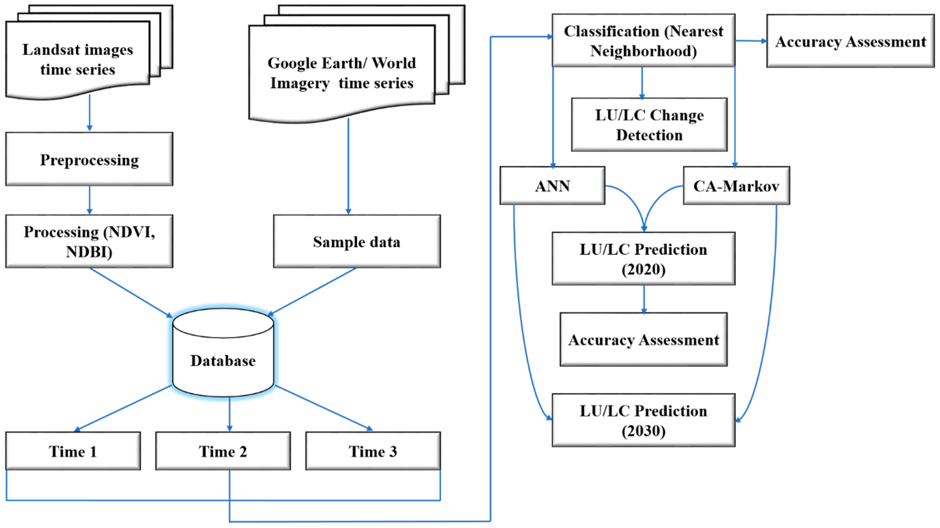
This study retrieved Landsat images (7 and 8) covering Urmia on 03/06/2000, 30/05/2010, and 02/06/2020. The images were downloaded from the USGS website. Initially, these images were pr-processed for geometric and radiometric corrections to make them suitable for information extraction. Then, in the categorization stage, high-resolution images (such as Google Earth and World Imagery), normalized difference built-up index (NDBI), and normalized difference vegetation index (NDVI) were used (sample points size are in Table 1) for choosing sample points from the old maps. In order to extract the LULC map, this study applied MLC due to its highest quality results compared to others [74]. Finally, predictions for the year 2030 were carried out with the methods detailed below, and their accuracy was investigated.

2.3. Methodology

2.3.1. CA–Markov

CA–Markov is a combined Cellular Automata/Markov Chain/Multicriteria/Multiobjective Land Allocation (MOLA) to predict the LULCC trends and characteristics over time [26,90,91]. CA model behaviors are influenced by the uncertainty stemming from the interaction between the model elements, structures, and quality of data sources that are considered model input. This model is often focused on the local interaction of the local cells, distinct spatial and temporal properties, and the rigorous computational ability of space that is proper for dynamic simulation and displays with self-made features. Thus, the CA model can be described as follows (Equation (1)):
S (t, t + 1) = f (S(t), N)
S is a collection of limited and discrete cellular models, N is a cellular field, t and t + 1 stand for different times, and f is the transformation of cellular states law in local space.
Markov chain is insufficient to actively simulate or predict LULC because it does not consider the spatial distribution in each land category or the growth direction [42,92]. CA–Markov is a Cellular Automata, Multiobjective Land Allocation predicting method that adds elements of spatial proximity and the knowledge of spatial distribution to the Markov chain [93,94,95,96,97,98].

2.3.2. Artificial Neural Network

To detect the probability of LULC transformation, ANN uses several output neurons to simulate LULC changes. In the first step, the neural network inputs are defined for the simulation. The simulation is cellular-based (pixel-based), and each cell has a set of natural features (spatial variables) as input to the neural network, defined as follows:
X = [x1, x2, x3... xi]T
where xi is the i-th property and T is the transition.
Each correlation between the spatial variables is evaluated by the mutual comparison of the raster, choosing the first raster from one variable and the second from the other. Next, the LULC region and the changes related to each group are measured between the initial and final times. In the next step, the probability of transformation through ANN is simulated. The neural network structure is created with three layers: the input layer, the latent layer, and the output layer. In the latent layer, the received signal by the j-th cell and netj (k,t) is calculated from the input layer for the k-th cell at t time and is defined as follows:
n e t j ( k , t ) = i w i , k x i   ( k , t )
wi,k is the weight between the input and latent layers, and x i (k,t) is the i-th saleable attribute related to i-th neuron in the latent layer according to the k-th cell at t time. The probability of relocation, with the performance of the output of a neural network being considered, is calculated as follows:
P ( k , t , l ) = Σ w j , l   1 1 + e n e t j ( k , t )
P(k,t,l) is the probability of changing from the current state of l LULC for k cell in t time, and wj,l is the weight between the latent and output layers [99].

2.3.3. Model Assessment

In this study, indices, including completeness, correctness, and quality, were used to quantitatively assess the forecast findings of these methods. The details of the indices used in the study are described below.
This index of completeness describes what percentages of the features shown in the source data are considered in the result. In this index, the feature units related to other features and distinguished wrongly have no impact on the value of this index. Therefore, this index is defined as follows:
Completeness   = ( TP / TP + FN ) 100
The correctness index is used for the correctness of classification. It refers to the percentage of the features that are detected in the results that are the same as the reference features. In this index, feature units that exist in the source data but that were not distinguished in the result do not influence the value of this index. This index is defined as follows:
Correctness = ( TP   /   FP + TP ) 100
The quality that pertains to the evaluation of the findings of both correctness and completeness and is thus defined as follows:
Quality   = ( TP / TP + FP + FN )   100
True positive (TP) is the number of units of features that exist in the source data and in the findings or the number of features that have been successfully detected correctly as a feature. False positive (FP) is the number of features that do not exist in the source data but have been identified in the results as a feature. False negative (FN) is the number of negative features that exist in source data but have not been identified in the results [100,101,102].
Figure 2 shows the research flowchart.

3. Results

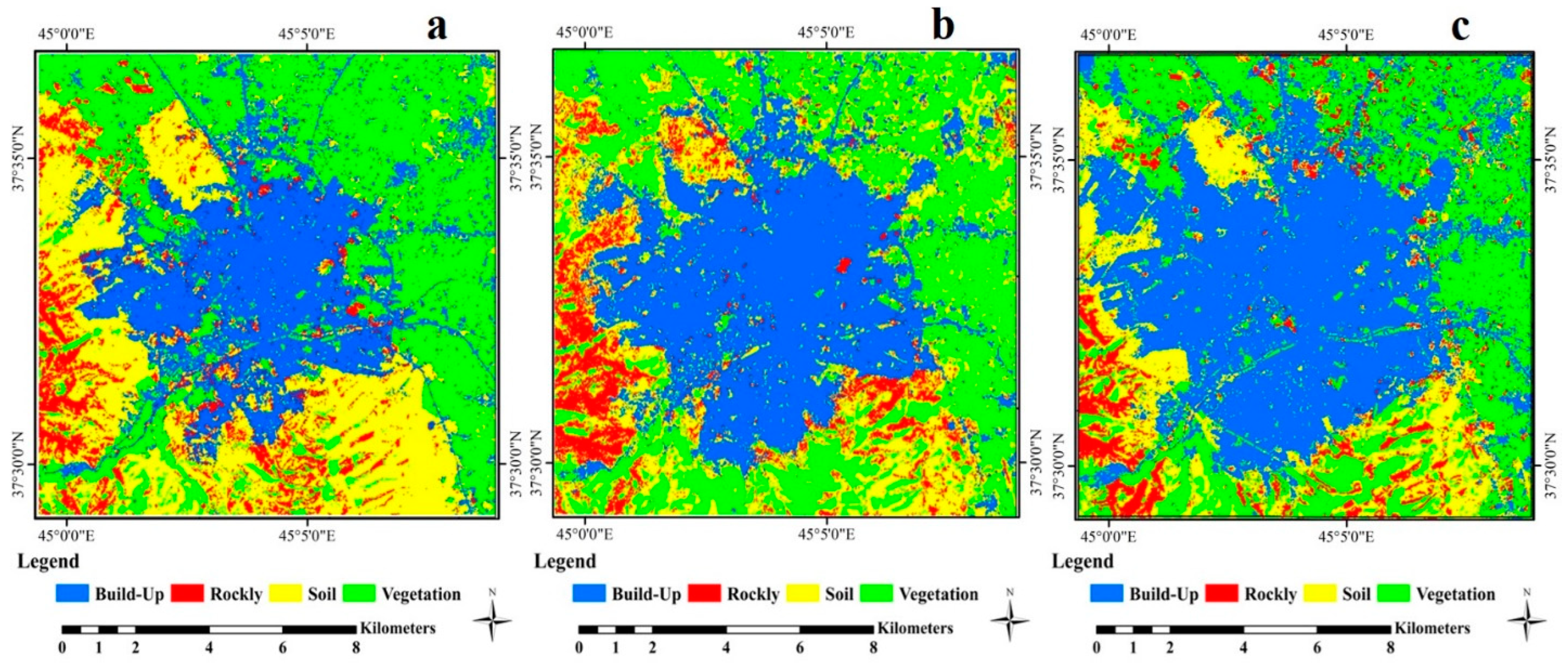
This section presents the findings of the methods used. Firstly, the findings of the classification with MLC are presented. Figure 3 shows the LULC maps obtained as a result of classification for 2000, 2010, and 2020.
Before using the achieved maps as the input of the LULC prediction methods, we needed verify each class’s classification. Table 2 depicts the result of the verification for the classification of each class in the three studied times. According to Table 2, the classification results in each of the three times appear suitable for all classes. The Kappa coefficient in all three times is higher than 90%, and in the 2020 map, it is approximately 100%. Although the accuracy for soil was less than 90% in 2000 and 2010, it is acceptable due to being above 83%. For accuracy assessment, the prepared maps were compared with the samples seen from Google Earth.
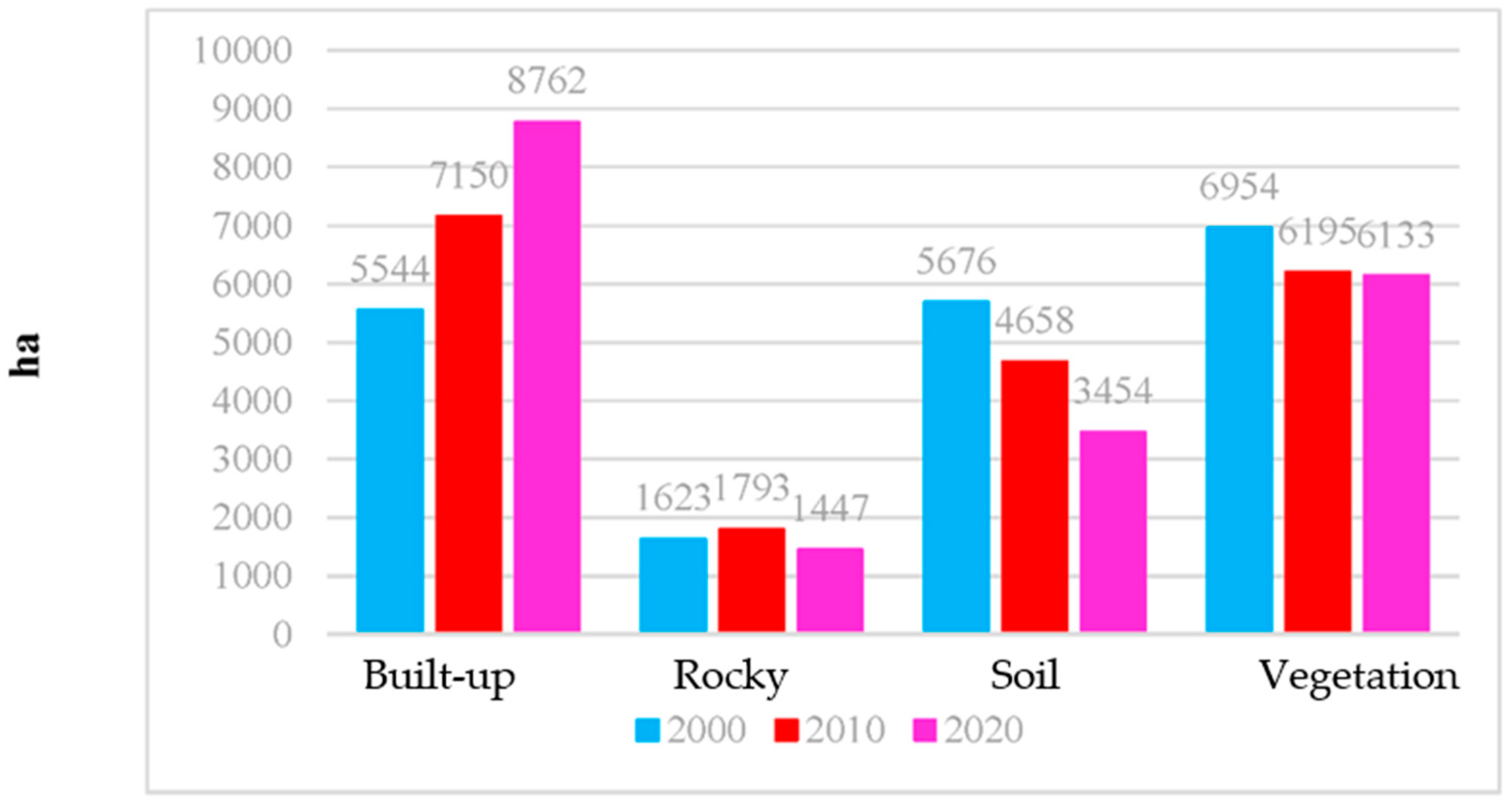
Figure 4 shows the changes in the area of LULC in different years. Urban LULC changed from 5500 hectares in 2000 to more than 7100 in 2010, exceeding 8700 in 2020. The figure shows that every ten years, almost 1600 hectares were added to the area of the urban LULC.
According to Figure 4, the rocky areas and vegetation changed little over the 20 years, but soil and built-up areas changes extensively. The soil class shrunk from 5700 hectares to 4650 in 2010 and to 3450 hectares in 2020. According to Figure 4, rocky areas increased in 2010 (the reduction of vegetation in rocky areas that had more vegetation in 2000; this could be due to logging in mountainous areas or decreased rainfall), but it decreased again in 2020.
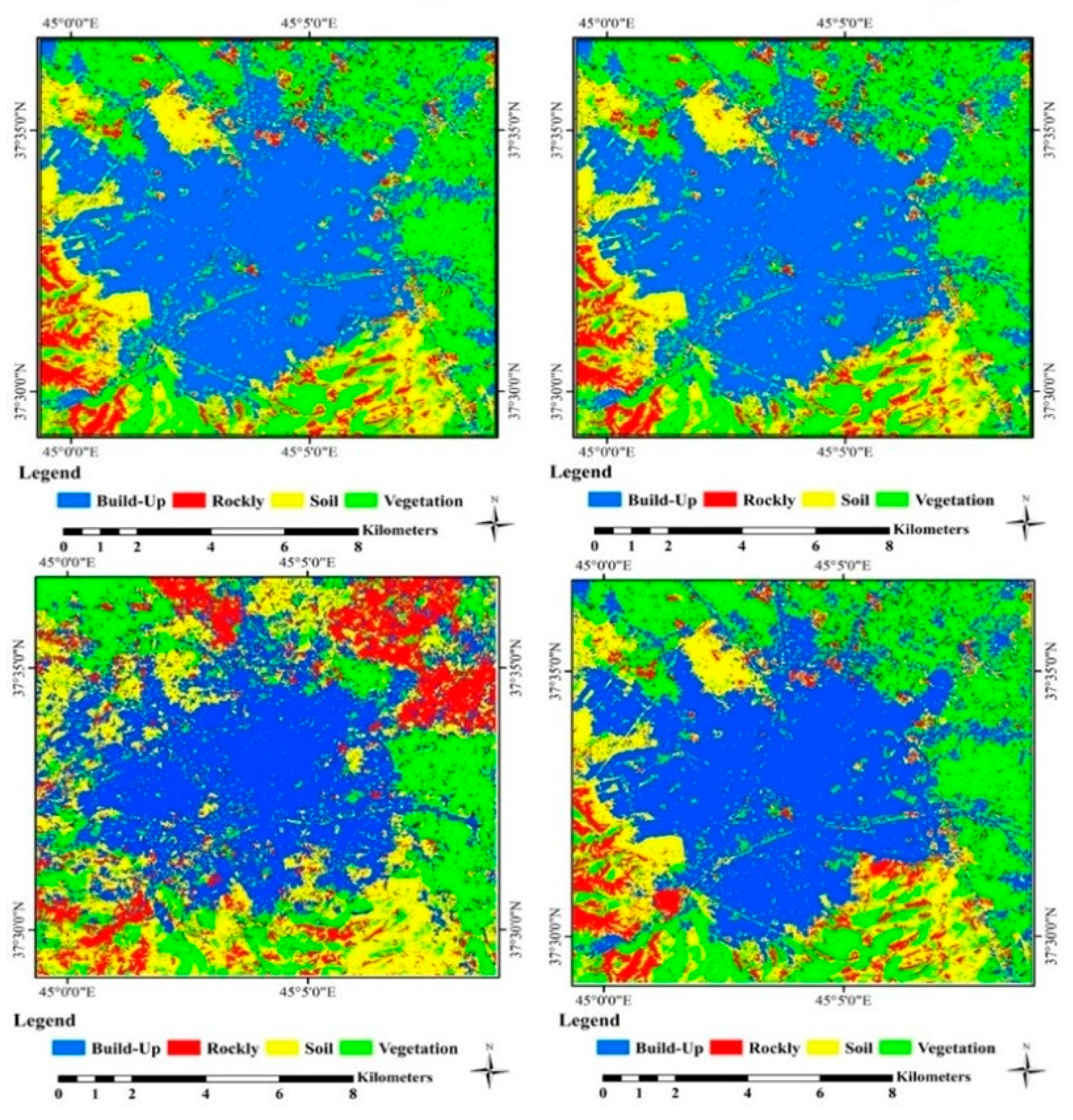
Figure 5 shows the comparison of the LULC for the 2020 map (a) obtained as a result of the classification with LULC prediction maps for 2020 as produced by the CA–Markov (b) and the ANN (c) method.
In the LULC classes shown in Figure 5, we can see that the appearance of the CA–Markov and ANN are pretty similar to the current situation. To better understand and compare the methods, the results of completeness, accuracy, and quality indicators are shown in Table 3.
Table 3 presents the completeness, correctness, and quality of the validation methods in order to evaluate and compare the outcomes of the LULC prediction with MLC for 2020. The blue numbers shown in the table indicate the most promising results. Accordingly, although the accuracy of the CA–Markov method was close to that of ANN in the LULC prediction models, the best results were obtained with the ANN technique. The ANN technique map had the lowest vicinity of rocky lands and, despite having the lowest completeness, had the highest correctness and forecast quality.
In the case of built-up areas, the CA–Markov method had the highest completeness and quality, while the ANN method had the highest correctness. For soil, the highest completeness and quality belonged to the ANN method, and the highest correctness belonged to the CA–Markov method. In the case of vegetation, the CA–Markov method had the best indices. In terms of average (all LU/LCs), the highest completeness and quality were achieved with ANN method, and the highest correctness with the CA–Markov method.
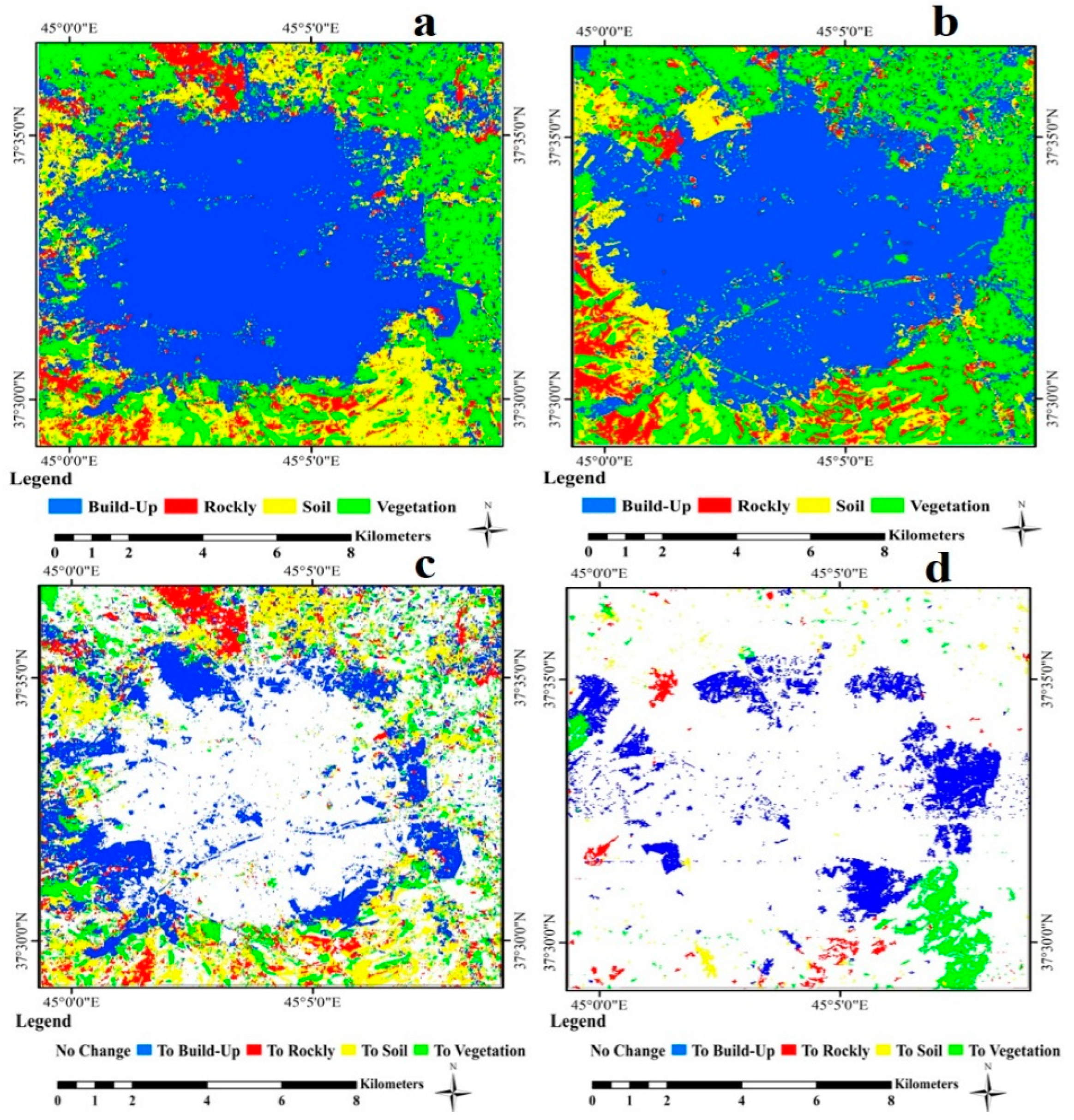
In conclusion, the results of the indices and subsequently, the typical mean of the two algorithms, ANN and CA–Markov, are very close to each other, but the ANN technique had the perfect mean in the two indices of completeness and quality, and the CA–Markov algorithm had the best correctness. Therefore, the urban and vegetation LU/LCs in the CA–Markov algorithm and the soil and rock LCs in the ANN algorithm were better simulated, as can be seen in Table 3. The most significant results of this research are that the CA–Markov algorithm is better able to predict those phenomena with wider and more continuous surfaces, while the ANN algorithm performs better in simulating phenomena that are smaller areas on the map and that include a lower percentage of the area. Figure 6 shows the LULC prediction map for 2030 of the CA–Markov and ANN (first row) and the map of changes in 2020–2030 (bottom row) as obtained by comparing the map predicted by the algorithms for 2030 and the LULC map for 2020 using MLC.
Figure 6 show that CA–Markov could reveal more changes compared to ANN. In both methods, the east side of the study region changes more than does the west side. To depict the degree of the LULC change, Figure 6 shows the area of each LULC in 2030.
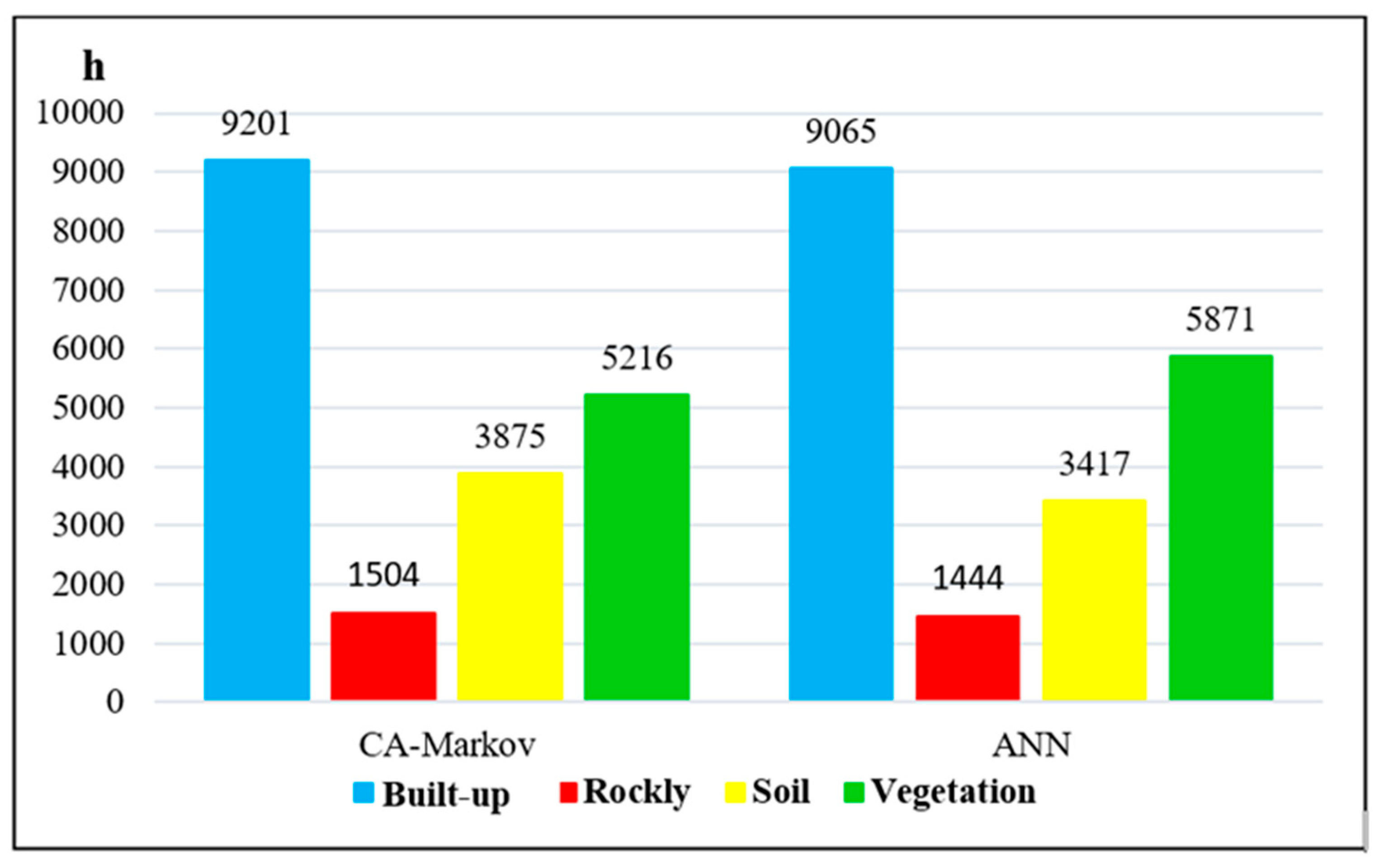
Figure 7 shows that, considering that the built-up LU area in this study will reach more than 9000 hectares in 2030, which is less than the 6000 hectares in 2000, the city of Urmia will extend by 50% over the next 30 years. Table 3 shows the area and the map of LULCs of urban (built-up) and vegetation as generated through CA–Markov, as well as the map and area of soil and rocky lands as generated through ANN. Figure 7 also shows that LU/LCs are similar in the area and more reliable in evaluation parameters (smaller zones in ANN and larger zones in CA–Markov).
Based on the two methods, the built-up environment appears to be growing, resulting in the decline of the vegetation area. The most significant difference in area between LU/LCs derived from the 2030 forecast algorithms is related to soil LC. It can be understood from the validation results of Table 3 that the precision, quality, and completeness statistics of this LU are lower than those of other LU/LCs, representing a significant statistical discrepancy between the algorithms.

4. Discussion

Today, the world is facing the challenge of environmental instability, which is the product of human activity. For example, one of the environmental concerns in the suburbs of Urmia is the drying up of a significant part of its lake [103,104,105]. Urban sprawl causes irreversible changes in the earth’s surface because even with the destruction of built-up areas, achieving a sustainable environment (natural environment) or one identical to what had been before construction is impossible. Therefore, managing urban sprawl is the most practical way to cope with this issue and can be accomplished by having reliable maps of the city expansion forecast. In this regard, various prediction methods such as CA–Markov and ANN have been employed in many regions all over the world, including the city of Thimphu, in Bhutan [106], the Majang Forest Biosphere Reserves of Gambella in southwestern Ethiopia [107], Orkhon Province in Mongolia [108], and the northeast of Iran [109]. However, unlike in these studies, in our study, which was conducted in the city of Urmia, two popular LULC prediction methods widely used in the literature were implemented and compared in a single study. Thus, this study comparing LULC prediction methods in Urmia significantly contributes to the literature.
This investigation indicated that the Urmia urban area has expanded too greatly [110]. It indicates that the built-up areas will occupy many natural and agricultural resources and that this land change situation threatens natural life [111]. It also confirmed the results of Zare-Naghadehi et al.’s study [74]. Table 2 shows that the evaluation of the accuracy of LULC maps is very suitable (except for soil in the 2000 and 2010 LULC maps). Moreover, comparing the methods revealed that both methods have a high capability to predict LULC; however, according to the evaluation criteria, ANN performed slightly better than did CA–Markov. Based on the results of this research, the CA–Markov algorithm is more accurate in predicting urban and vegetation areas, while the ANN algorithm is more accurate in predicting soil and rock cover.
The first thing that should be considered for a reliable prediction is the accuracy of the input data. Table 2 shows that the average accuracy of the built-up class classification is 97.47%, which is high. Furthermore, by examining other classes, it is clear that the accuracy of classification with MLC is quite suitable as an input for predicting changes (only the accuracy of the soil class in the 2000 and 2010 maps is less than 90%).
Examining the change and transformation of LULC (Figure 4) shows that over 20 years (2000–2020), the area of the city grew by nearly 60%, which means the loss of other classes of LULCs. During this time, bare soil decreased to about 61% of its area (a loss of 2222 hectares during the study). Additionally, more than 800 hectares of vegetation cover were lost, meaning that there is low environmental stability in the area. In short, Table 3 presents the main results of this study: three indicators were used to assess the effectiveness of the CA–Markov and ANN methods and revealed that both algorithms have high capabilities for LULC prediction. Although, according to the results in Table 3, the more accurate prediction was achieved by ANN, the CA–Markov algorithm’s performance regarding urban sprawl, which is the focus of this study, performed better than did ANN in two indicators (completeness and quality) for predicting build-up.

5. Conclusions

Urban sprawl can prevent sustainable development goals and cause considerable impairment, especially in the suburbs, which are more vulnerable to changes because of human exploitation. Moreover, predicting the urban development pattern and the region’s changes can be crucial for urban investors, residents, and landowners, highlighting the importance of LULCC analysis. Therefore, the timely and efficient decisions are essential but impossible to make without accurate information. More specifically, a proper LULC map will pave the road for local planners and decision-makers to monitor environmental hazards such as soil erosion, flooding, landslides, and degradation of pastures. To this end, Landsat images with a long imaging record can be an excellent archive to research the shift in an area’s LULC. Furthermore, various algorithms exist to forecast LU and are slightly or generally different from each other in their structures. Knowing which algorithm functions better can help researchers use the most efficient one in their future research.
Due to its high development rate in recent years, this study was conducted in Urmia to evaluate and compare two common algorithms (CA–Markov and ANN) and recognize which has the better performance. Consequently, researchers and authorities can use the most efficient one in future research and projects. For this purpose, satellite images were used to assess four land-use (constructed, rocky areas, vegetation cover, and soil) in Urmia in 2000, 2010, and 2020, and their LULC images were obtained. Then, the results of the CA–Markov and ANN algorithms were compared, indicating that all parameters in the two algorithms were higher than 90% (96.47 correctness in the CA–Markov algorithm and 96.21 completeness and 93.8 quality in the ANN algorithm) and that these algorithms have excellent prediction ability. Preliminary findings from the LULC map indicate that the city’s growth was positive, while on the other hand, the areas covered by soil and vegetation were limited, and the rocky areas almost remained unchanged. The CA–Markov algorithm had the highest completeness for rock cover, and the ANN algorithm, which shows rocky terrain with less accuracy, had low completeness but high correctness and quality. On the other hand, in soil land cover, the ANN method had the highest completeness and quality, while the CA–Markov algorithm had the highest correctness. However, in vegetation, all three statistics pointed to the superiority of the CA–Markov method. Regarding the average criteria used in all LULCs, the CA–Markov algorithm had the highest completeness, and the ANN algorithm had the highest correctness and quality.
In summary, both CA–Markov and the ANN algorithms perform well in a way that one cannot decide which algorithm excels over the other, and thus more testing is required. However, the limitation of the study is that there is insufficient research comparing different prediction models in other regions to achieve a more comprehensive view of their efficiency and accuracy. Therefore, although the CA–Markov method is more effective in predicting LULCs in extensive areas and the ANN method is more effective for smaller areas, we suggest that other researchers evaluate other algorithms in other regions to better understand these prediction models. We also recommend that researchers compare the results from other methods, such as the Genetic Algorithm Optimized Neural Network Model [112], CA-Based SLEUTH [113], and CycleGANs-based CNN [114], using several evaluation indices.

Author Contributions

Conceptualization, A.O.-N.; Formal analysis, M.A.; Resources, S.S.-A.; Writing—original draft, S.-S.S. and F.H.; Writing—review & editing, M.A.; Supervision, A.O.-N. and J.L.V.G. All authors have read and agreed to the published version of the manuscript.

Funding

This research received no external funding.

Institutional Review Board Statement

Not applicable.

Informed Consent Statement

Not applicable.

Data Availability Statement

All date are freely available from the LANDSAT.

Conflicts of Interest

The authors declare no conflict of interest.

References

  1. Bebbington, J. Sustainable development: A review of the international development, business and accounting literature. In Accounting Forum; Taylor & Francis: Oxfordshire, UK, 2001. [Google Scholar]
  2. Budd, W.; Lovrich, N.; Pierce, J.C.; Chamberlain, B. Cultural sources of variations in US urban sustainability attributes. Cities 2008, 25, 257–267. [Google Scholar] [CrossRef]
  3. Bovet, J.; Reese, M.; Köck, W. Taming expansive land use dynamics—Sustainable land use regulation and urban sprawl in a comparative perspective. Land Use Policy 2018, 77, 837–845. [Google Scholar] [CrossRef]
  4. Hassan, A.M.; Lee, H. Toward the sustainable development of urban areas: An overview of global trends in trials and policies. Land Use Policy 2015, 48, 199–212. [Google Scholar] [CrossRef]
  5. Rubiera-Morollón, F.; Garrido-Yserte, R. Recent Literature about Urban Sprawl: A Renewed Relevance of the Phenomenon from the Perspective of Environmental Sustainability. Sustainability 2020, 12, 6551. [Google Scholar] [CrossRef]
  6. Coq-Huelva, D.; Asián-Chaves, R. Urban Sprawl and Sustainable Urban Policies. A Review of the Cases of Lima, Mexico City and Santiago de Chile. Sustainability 2019, 11, 5835. [Google Scholar] [CrossRef] [Green Version]
  7. Artmann, M.; Inostroza, L.; Fan, P. Urban sprawl, compact urban development and green cities. How much do we know, how much do we agree? Ecol. Indic. 2018, 96, 3–9. [Google Scholar] [CrossRef]
  8. Shao, Z.; Sumari, N.S.; Portnov, A.; Ujoh, F.; Musakwa, W.; Mandela, P.J. Urban sprawl and its impact on sustainable urban development: A combination of remote sensing and social media data. Geospat. Inf. Sci. 2020, 24, 241–255. [Google Scholar] [CrossRef]
  9. Næss, P. Central dimensions in a sustainable urban development. Sustain. Dev. 1995, 3, 120–129. [Google Scholar] [CrossRef]
  10. Mansouri Daneshvar, M.R.; Rabbani, G.; Shirvani, S. Assessment of urban sprawl effects on regional climate change using a hybrid model of factor analysis and analytical network process in the Mashhad city, Iran. Environ. Syst. Res. 2019, 8, 1–12. [Google Scholar]
  11. Aliyu, A.A.; Amadu, L. Urbanization, cities, and health: The challenges to Nigeria—A review. Ann. Afr. Med. 2017, 16, 149. [Google Scholar] [CrossRef]
  12. Vani, M.; Prasad, P.R.C. Assessment of spatio-temporal changes in land use and land cover, urban sprawl, and land surface temperature in and around Vijayawada city, India. Environ. Dev. Sustain. 2020, 22, 3079–3095. [Google Scholar] [CrossRef]
  13. Henderson, V. Urbanization in developing countries. World Bank Res. Obs. 2002, 17, 89–112. [Google Scholar] [CrossRef]
  14. Hatab, A.A.; Cavinato, M.E.R.; Lindemer, A.; Lagerkvist, C.J. Urban sprawl, food security and agricultural systems in developing countries: A systematic review of the literature. Cities 2019, 94, 129–142. [Google Scholar] [CrossRef]
  15. Nijhoff, M. Urbanization in Developing Countries; Springer: Cham, Switzerland, 2013. [Google Scholar]
  16. Bonan, G.B. Forests and climate change: Forcings, feedbacks, and the climate benefits of forests. Science 2008, 320, 1444–1449. [Google Scholar] [CrossRef] [PubMed] [Green Version]
  17. Pflugmacher, D.; Rabe, A.; Peters, M.; Hostert, P. Mapping pan-European land cover using Landsat spectral-temporal metrics and the European LUCAS survey. Remote Sens. Environ. 2019, 221, 583–595. [Google Scholar] [CrossRef]
  18. Anderson, K.; Ryan, B.; Sonntag, W.; Kavvada, A.; Friedl, L. Earth observation in service of the 2030 Agenda for Sustainable Development. Geo-spat. Inf. Sci. 2017, 20, 77–96. [Google Scholar] [CrossRef]
  19. Feddema, J.J.; Oleson, K.W.; Bonan, G.B.; Mearns, L.O.; Buja, L.E.; Meehl, G.A.; Washington, W.M. The Importance of Land-Cover Change in Simulating Future Climates. Science 2005, 310, 1674–1678. [Google Scholar] [CrossRef] [PubMed] [Green Version]
  20. Liu, J.; Liu, M.; Tian, H.; Zhuang, D.; Zhang, Z.; Zhang, W.; Tang, X.; Deng, X. Spatial and temporal patterns of China’s cropland during 1990–2000: An analysis based on Landsat TM data. Remote Sens. Environ. 2005, 98, 442–456. [Google Scholar] [CrossRef]
  21. Luo, G.; Zhou, C.; Chen, X. Process of land use/land cover change in the oasis of arid region. Acta Geogr. Sin. Chin. Ed. 2003, 58, 63–72. [Google Scholar]
  22. Maleki, M.; Van Genderen, J.L.; Tavakkoli-Sabour, S.M.; Saleh, S.S.; Babaee, E. Land use/cover change in Dinevar rural area of West Iran during 2000–2018 and its prediction for 2024 and 2030. Geomatics Appl. Geogr. 2020, 15, 93–105. [Google Scholar] [CrossRef]
  23. Tang, J.; Li, Y.; Cui, S.; Xu, L.; Ding, S.; Nie, W. Linking land-use change, landscape patterns, and ecosystem services in a coastal watershed of southeastern China. Glob. Ecol. Conserv. 2020, 23, e01177. [Google Scholar] [CrossRef]
  24. Wang, X.; Zheng, Y.; Li, S. Analysis of land use and landscape pattern change in west of Hainan Island. J. Desert Res. 2006, 26, 409–414. [Google Scholar]
  25. Abuelaish, B.; Olmedo, M.T.C. Scenario of land use and land cover change in the Gaza Strip using remote sensing and GIS models. Arab. J. Geosci. 2016, 9, 274. [Google Scholar] [CrossRef]
  26. Islam, K.; Jashimuddin, M.; Nath, B.; Nath, T.K. Land use classification and change detection by using multi-temporal remotely sensed imagery: The case of Chunati wildlife sanctuary, Bangladesh. Egypt. J. Remote. Sens. Space Sci. 2018, 21, 37–47. [Google Scholar] [CrossRef]
  27. Subedi, P.; Subedi, K.; Thapa, B. Application of a hybrid cellular automaton–markov (ca-markov) model in land-use change prediction: A case study of saddle creek drainage basin, Florida. Appl. Ecol. Environ. Sci. 2013, 1, 126–132. [Google Scholar] [CrossRef] [Green Version]
  28. Pindozzi, S.; Cervelli, E.; Recchi, P.F.; Capolupo, A.; Boccia, L. Predicting land use change on a broad area: Dyna-CLUE model application to the Litorale Domizio-Agro Aversano (Campania, South Italy). J. Agric. Eng. 2017, 48, 27. [Google Scholar] [CrossRef]
  29. Turner, B.L.; Lambin, E.F., II; Reenberg, A. The emergence of land change science for global environmental change and sustainability. Proc. Natl. Acad. Sci. USA 2007, 104, 20666–20671. [Google Scholar] [CrossRef] [Green Version]
  30. Foley, J.A.; DeFries, R.; Asner, G.P.; Barford, C.; Bonan, G.; Carpenter, S.R.; Chapin, F.S.; Coe, M.T.; Daily, G.C.; Gibbs, H.K.; et al. Global consequences of land use. Science 2005, 309, 570–574. [Google Scholar] [CrossRef] [PubMed] [Green Version]
  31. Hamad, R.; Balzter, H.; Kolo, K. Predicting Land Use/Land Cover Changes Using a CA-Markov Model under Two Different Scenarios. Sustainability 2018, 10, 3421. [Google Scholar] [CrossRef] [Green Version]
  32. Roy, S.; Farzana, K.; Papia, M.; Hasan, M. Monitoring and prediction of land use/land cover change using the integration of Markov chain model and cellular automation in the Southeastern Tertiary Hilly Area of Bangladesh. Int. J. Sci. Basic Appl. Res. 2015, 24, 125–148. [Google Scholar]
  33. de Almeida, A.S.; Vieira, I.C.G.; Ferraz, S.F.B. Long-term assessment of oil palm expansion and landscape change in the eastern Brazilian Amazon. Land Use Policy 2020, 90, 104321. [Google Scholar] [CrossRef]
  34. Aghimien, D.O.; Aigbavboa, C.; Edwards, D.J.; Mahamadu, A.-M.; Olomolaiye, P.; Nash, H.; Onyia, M. A fuzzy synthetic evaluation of the challenges of smart city development in developing countries. Smart Sustain. Built Environ. 2020, 11, 405–421. [Google Scholar] [CrossRef]
  35. Bawa, M.; Cagáňová, D.; Szilva, I.; Spirkova, D. Importance of Internet of Things and Big Data in Building Smart City and What Would Be Its Challenges; Springer: Cham, Switzerland, 2016; pp. 605–616. [Google Scholar] [CrossRef]
  36. Komolafe, A.A.; Awe, B.S.; Olorunfemi, I.E.; Oguntunde, P.G. Modelling flood-prone area and vulnerability using integration of multi-criteria analysis and HAND model in the Ogun River Basin, Nigeria. Hydrol. Sci. J. 2020, 65, 1766–1783. [Google Scholar] [CrossRef]
  37. Jat, M.K.; Choudhary, M.; Saxena, A. Application of geo-spatial techniques and cellular automata for modelling urban growth of a heterogeneous urban fringe. Egypt. J. Remote Sens. Space Sci. 2017, 20, 223–241. [Google Scholar] [CrossRef]
  38. Tadese, M.; Kumar, L.; Koech, R.; Kogo, B.K. Mapping of land-use/land-cover changes and its dynamics in Awash River Basin using remote sensing and GIS. Remote Sens. Appl. Soc. Environ. 2020, 19, 100352. [Google Scholar] [CrossRef]
  39. Nugroho, F.; Al-Sanjary, O.I. A Review of Simulation Urban Growth Model. Int. J. Eng. Technol. 2018, 7, 17–23. [Google Scholar] [CrossRef]
  40. Otuoze, S.; Hunt, D.; Jefferson, I. Neural Network Approach to Modelling Transport System Resilience for Major Cities: Case Studies of Lagos and Kano (Nigeria). Sustainability 2021, 13, 1371. [Google Scholar] [CrossRef]
  41. Dutta, D.; Rahman, A.; Paul, S.K.; Kundu, A. Estimating urban growth in peri-urban areas and its interrelationships with built-up density using earth observation datasets. Ann. Reg. Sci. 2020, 65, 67–82. [Google Scholar] [CrossRef]
  42. Mansour, S.; Al-Belushi, M.; Al-Awadhi, T. Monitoring land use and land cover changes in the mountainous cities of Oman using GIS and CA-Markov modelling techniques. Land Use Policy 2020, 91, 104414. [Google Scholar] [CrossRef]
  43. Hale, C. Economic marginalization, social exclusion, and crime. In Criminology; Oxford University Press: Oxford, UK, 2013; pp. 289–307. [Google Scholar]
  44. Nayak, P.K.; Oliveira, L.E.; Berkes, F. Resource degradation, marginalization, and poverty in small-scale fisheries: Threats to social-ecological resilience in India and Brazil. Ecol. Soc. 2014, 19. [Google Scholar] [CrossRef] [Green Version]
  45. Foody, G.M. Status of land cover classification accuracy assessment. Remote Sens. Environ. 2002, 80, 185–201. [Google Scholar] [CrossRef]
  46. Green, K.; Kempka, D.; Lackey, L. Using remote sensing to detect and monitor land-cover and land-use change. Photogramm. Eng. Remote Sens. 1994, 60, 331–337. [Google Scholar]
  47. Hütt, C.; Koppe, W.; Miao, Y.; Bareth, G. Best Accuracy Land Use/Land Cover (LULC) Classification to Derive Crop Types Using Multitemporal, Multisensor, and Multi-Polarization SAR Satellite Images. Remote Sens. 2016, 8, 684. [Google Scholar] [CrossRef] [Green Version]
  48. Duan, Y.; Wang, X.; Wei, Y. Land use change analysis of Daishan Island using multi-temporal remote sensing imagery. Arab. J. Geosci. 2020, 13, 741. [Google Scholar] [CrossRef]
  49. Keshtkar, H.; Voigt, W.; Alizadeh, E. Land-cover classification and analysis of change using machine-learning classifiers and multi-temporal remote sensing imagery. Arab. J. Geosci. 2017, 10, 154. [Google Scholar] [CrossRef]
  50. Kolli, M.; Opp, C.; Karthe, D.; Groll, M. Mapping of Major Land-Use Changes in the Kolleru Lake Freshwater Ecosystem by Using Landsat Satellite Images in Google Earth Engine. Water 2020, 12, 2493. [Google Scholar] [CrossRef]
  51. Dadashpoor, H.; Salarian, F. Urban sprawl on natural lands: Analyzing and predicting the trend of land use changes and sprawl in Mazandaran city region, Iran. Environ. Dev. Sustain. 2018, 22, 593–614. [Google Scholar] [CrossRef]
  52. Mc Cutchan, M.; Özdal-Oktay, S.; Giannopoulos, I. Semantic-based urban growth prediction. Trans. GIS 2020, 24, 1482–1503. [Google Scholar] [CrossRef]
  53. Veldkamp, A.; Lambin, E.F. Predicting land-use change. Agric. Ecosyst. Environ. 2001, 85, 1–6. [Google Scholar] [CrossRef]
  54. Mishra, V.N.; Rai, P.K. A remote sensing aided multi-layer perceptron-Markov chain analysis for land use and land cover change prediction in Patna district (Bihar), India. Arab. J. Geosci. 2016, 9, 249. [Google Scholar] [CrossRef]
  55. Arsanjani, J.J.; Helbich, M.; Kainz, W.; Boloorani, A.D. Integration of logistic regression, Markov chain and cellular automata models to simulate urban expansion. Int. J. Appl. Earth Obs. Geoinform. 2013, 21, 265–275. [Google Scholar] [CrossRef]
  56. Mustafa, A.; Ebaid, A.; Omrani, H.; McPhearson, T. A multi-objective Markov Chain Monte Carlo cellular automata model: Simulating multi-density urban expansion in NYC. Comput. Environ. Urban Syst. 2021, 87, 101602. [Google Scholar] [CrossRef]
  57. Kisamba, F.C.; Li, F. Analysis and modelling urban growth of Dodoma urban district in Tanzania using an integrated CA–Markov model. GeoJournal 2022, 1–22. [Google Scholar] [CrossRef]
  58. Buya, S.; Tongkumchum, P.; Owusu, B.E. Modelling of land-use change in Thailand using binary logistic regression and multinomial logistic regression. Arab. J. Geosci. 2020, 13, 437. [Google Scholar] [CrossRef]
  59. Tayyebi, A.R.; Yazdanpanah, M.J.; Pijanowski, B.C.; Saeedi, S.; Tayyebi, A.H. A spatial logistic regression model for simulating land use patterns: A case study of the Shiraz Metropolitan area of Iran. In Advances in Earth Observation of Global Change; Springer: Dordrecht, The Netherlands, 2010; pp. 27–42. [Google Scholar]
  60. Munthali, M.; Mustak, S.; Adeola, A.; Botai, J.; Singh, S.; Davis, N. Modelling land use and land cover dynamics of Dedza district of Malawi using hybrid Cellular Automata and Markov model. Remote Sens. Appl. Soc. Environ. 2019, 17, 100276. [Google Scholar] [CrossRef]
  61. Wang, X.; Li, J.; Zheng, T.; Diao, S.; Zhang, X.; Tian, Y. Constructing Landscape Ecological Security Patterns of an Ancient Capital Based on Cellular Automata Theory. Urban Sci. 2022, 6, 29. [Google Scholar] [CrossRef]
  62. Jantz, A.C.; Goetz, S.J.; Shelley, M.K. Using the Sleuth Urban Growth Model to Simulate the Impacts of Future Policy Scenarios on Urban Land Use in the Baltimore-Washington Metropolitan Area. Environ. Plan. B Plan. Des. 2004, 31, 251–271. [Google Scholar] [CrossRef]
  63. Saxena, A.; Jat, M.K. Capturing heterogeneous urban growth using SLEUTH model. Remote Sens. Appl. Soc. Environ. 2019, 13, 426–434. [Google Scholar] [CrossRef]
  64. Al Rifat, S.A.; Liu, W. Predicting future urban growth scenarios and potential urban flood exposure using Artificial Neural Network-Markov Chain model in Miami Metropolitan Area. Land Use Policy 2022, 114, 105994. [Google Scholar] [CrossRef]
  65. Kim, K.-D.; Lee, S.; Oh, H.-J. Prediction of ground subsidence in Samcheok City, Korea using artificial neural networks and GIS. Environ. Earth Sci. 2009, 58, 61–70. [Google Scholar] [CrossRef]
  66. Chen, Y.; Huang, L. Modeling growth curve of fractal dimension of urban form of Beijing. Phys. A Stat. Mech. Its Appl. 2019, 523, 1038–1056. [Google Scholar] [CrossRef] [Green Version]
  67. Chen, Y.-G. Logistic models of fractal dimension growth of urban morphology. Fractals 2018, 26, 1850033. [Google Scholar] [CrossRef] [Green Version]
  68. Baqa, M.; Chen, F.; Lu, L.; Qureshi, S.; Tariq, A.; Wang, S.; Jing, L.; Hamza, S.; Li, Q. Monitoring and Modeling the Patterns and Trends of Urban Growth Using Urban Sprawl Matrix and CA-Markov Model: A Case Study of Karachi, Pakistan. Land 2021, 10, 700. [Google Scholar] [CrossRef]
  69. Mondal, M.S.; Sharma, N.; Garg, P.K.; Kappas, M. Statistical independence test and validation of CA Markov land use land cover (LULC) prediction results. Egypt. J. Remote Sens. Space Sci. 2016, 19, 259–272. [Google Scholar] [CrossRef]
  70. Yi, S.; Zhou, Y.; Li, Q. A New Perspective for Urban Development Boundary Delineation Based on the MCR Model and CA-Markov Model. Land 2022, 11, 401. [Google Scholar] [CrossRef]
  71. Zhou, L.; Dang, X.; Sun, Q.; Wang, S. Multi-scenario simulation of urban land change in Shanghai by random forest and CA-Markov model. Sustain. Cities Soc. 2020, 55, 102045. [Google Scholar] [CrossRef]
  72. Girma, R.; Fürst, C.; Moges, A. Land use land cover change modeling by integrating artificial neural network with cellular Automata-Markov chain model in Gidabo river basin, main Ethiopian rift. Environ. Challenges 2022, 6, 106034. [Google Scholar] [CrossRef]
  73. Malik, A.; Bhagwat, A. Modelling groundwater level fluctuations in urban areas using artificial neural network. Groundw. Sustain. Dev. 2021, 12, 100484. [Google Scholar] [CrossRef]
  74. Naghadehi, S.Z.; Asadi, M.; Maleki, M.; Tavakkoli-Sabour, S.-M.; Van Genderen, J.; Saleh, S.-S. Prediction of Urban Area Expansion with Implementation of MLC, SAM and SVMs’ Classifiers Incorporating Artificial Neural Network Using Landsat Data. ISPRS Int. J. Geo-Inf. 2021, 10, 513. [Google Scholar] [CrossRef]
  75. Wang, Y.; Sha, Z.; Tan, X.; Lan, H.; Liu, X.; Rao, J. Modeling urban growth by coupling localized spatio-temporal association analysis and binary logistic regression. Comput. Environ. Urban Syst. 2020, 81, 101482. [Google Scholar] [CrossRef]
  76. Xu, E.; Chen, Y. Modeling Intersecting Processes of Wetland Shrinkage and Urban Expansion by a Time-Varying Methodology. Sustainability 2019, 11, 4953. [Google Scholar] [CrossRef] [Green Version]
  77. Kaviari, F.; Mesgari, M.S.; Seidi, E.; Motieyan, H. Simulation of urban growth using agent-based modeling and game theory with different temporal resolutions. Cities 2019, 95, 102387. [Google Scholar] [CrossRef]
  78. Xu, T.; Gao, J.; Coco, G.; Wang, S. Urban expansion in Auckland, New Zealand: A GIS simulation via an intelligent self-adapting multiscale agent-based model. Int. J. Geogr. Inf. Sci. 2020, 34, 2136–2159. [Google Scholar] [CrossRef]
  79. Yatoo, S.A.; Sahu, P.; Kalubarme, M.H.; Kansara, B.B. Monitoring land use changes and its future prospects using cellular automata simulation and artificial neural network for Ahmedabad city, India. GeoJournal 2020, 87, 765–786. [Google Scholar] [CrossRef]
  80. Khaledi, S.; Ghahroodi, T.M. Measuring and evaluating the resilience of urban areas against urban flooding (Case study: Urmia City). Sustain. Develop. Geograph. Environ. 2019, 2, 169–182. [Google Scholar] [CrossRef]
  81. Chitsazan, M.; Aghazadeh, N.; Mirzaee, Y.; Golestan, Y. Hydrochemical characteristics and the impact of anthropogenic activity on groundwater quality in suburban area of Urmia city, Iran. Environ. Dev. Sustain. 2019, 21, 331–351. [Google Scholar] [CrossRef]
  82. Abedini, A.; Khalili, A.; Asadi, N. Urban Sprawl Evaluation Using Landscape Metrics and Black-and-White Hypothesis (Case Study: Urmia City). J. Indian Soc. Remote Sens. 2020, 48, 1021–1034. [Google Scholar] [CrossRef]
  83. Abedini, A.; Khalili, A. Determining the capacity infill development in growing metropolitans: A case study of Urmia city. J. Urban Manag. 2019, 8, 316–327. [Google Scholar] [CrossRef]
  84. Gharakhanlou, N.M.; Hooshangi, N. Spatio-temporal simulation of the novel coronavirus (COVID-19) outbreak using the agent-based modeling approach (case study: Urmia, Iran). Informatics Med. Unlocked 2020, 20, 100403. [Google Scholar] [CrossRef]
  85. Khedmatzadeh, A.; Mousavi, M.N.; Torkamani, H.M. An Analysis on Land Use Process Changes and Forecasting in Urmia City Using SVM Model and Neural Networks. J. Remote Sens. Gis 2021, 12, 53–72. [Google Scholar] [CrossRef]
  86. Mohammadi, A.; Ghassoun, Y.; Löwner, M.-O.; Behmanesh, M.; Faraji, M.; Nemati, S.; Toolabi, A.; Abdolahnejad, A.; Panahi, H.; Heydari, H.; et al. Spatial analysis and risk assessment of urban BTEX compounds in Urmia, Iran. Chemosphere 2020, 246, 125769. [Google Scholar] [CrossRef] [PubMed]
  87. Abedini, A. Measurement of Urban Sprawl Using Spatial-temporal Data (Case Study: City of Urmia). Motaleate Shahri 2018, 7, 63–76. [Google Scholar]
  88. Abedini, A.; Mosayebzade, A.; Shokrani, M. Urban Physical Development of Urmia City by Quantitative Models. Hum. Geogr. Res. 2015, 47, 411–422. [Google Scholar]
  89. Takada, T.; Miyamoto, A.; Hasegawa, S.F. Derivation of a yearly transition probability matrix for land-use dynamics and its applications. Landsc. Ecol. 2010, 25, 561–572. [Google Scholar] [CrossRef]
  90. Nath, B.; Niu, Z.; Singh, R.P. Land Use and Land Cover Changes, and Environment and Risk Evaluation of Dujiangyan City (SW China) Using Remote Sensing and GIS Techniques. Sustainability 2018, 10, 4631. [Google Scholar] [CrossRef] [Green Version]
  91. Nouri, J.; Gharagozlou, A.; Arjmandi, R.; Faryadi, S.; Adl, M. Predicting Urban Land Use Changes Using a CA–Markov Model. Arab. J. Sci. Eng. 2014, 39, 5565–5573. [Google Scholar] [CrossRef]
  92. Ghosh, P.; Mukhopadhyay, A.; Chanda, A.; Mondal, P.; Akhand, A.; Mukherjee, S.; Nayak, S.; Ghosh, S.; Mitra, D.; Ghosh, T.; et al. Application of Cellular automata and Markov-chain model in geospatial environmental modeling- A review. Remote Sens. Appl. Soc. Environ. 2017, 5, 64–77. [Google Scholar] [CrossRef]
  93. Lin, Z.; Peng, S. Comparison of multimodel simulations of land use and land cover change considering integrated constraints—A case study of the Fuxian Lake basin. Ecol. Indic. 2022, 142, 109254. [Google Scholar] [CrossRef]
  94. Matlhodi, B.; Kenabatho, P.; Parida, B.; Maphanyane, J. Analysis of the Future Land Use Land Cover Changes in the Gaborone Dam Catchment Using CA-Markov Model: Implications on Water Resources. Remote Sens. 2021, 13, 2427. [Google Scholar] [CrossRef]
  95. Mubako, S.; Nnko, H.J.; Peter, K.H.; Msongaleli, B. Evaluating historical and predicted long-term land use/land-cover change in Dodoma Urban District, Tanzania: 1992. Phys. Chem. Earth, Parts ABC 2022, 128, 103205. [Google Scholar] [CrossRef]
  96. Nath, B.; Wang, Z.; Ge, Y.; Islam, K.; Singh, R.P.; Niu, Z. Land Use and Land Cover Change Modeling and Future Potential Landscape Risk Assessment Using Markov-CA Model and Analytical Hierarchy Process. ISPRS Int. J. Geo-Inf. 2020, 9, 134. [Google Scholar] [CrossRef] [Green Version]
  97. Rahman, M.T.U.; Tabassum, F.; Rasheduzzaman, M.; Saba, H.; Sarkar, L.; Ferdous, J.; Uddin, S.Z.; Islam, A.Z.M.Z. Temporal dynamics of land use/land cover change and its prediction using CA-ANN model for southwestern coastal Bangladesh. Environ. Monit. Assess. 2017, 189, 565. [Google Scholar] [CrossRef] [PubMed]
  98. Sang, L.; Zhang, C.; Yang, J.; Zhu, D.; Yun, W. Simulation of land use spatial pattern of towns and villages based on CA–Markov model. Math. Comput. Model. 2011, 54, 938–943. [Google Scholar] [CrossRef]
  99. Saputra, M.H.; Lee, H.S. Prediction of Land Use and Land Cover Changes for North Sumatra, Indonesia, Using an Artificial-Neural-Network-Based Cellular Automaton. Sustainability 2019, 11, 3024. [Google Scholar] [CrossRef] [Green Version]
  100. Maleki, M.; Sabour, S.M.T.; Rahmati, M.; Arjomand, B. Statistical Integration of Radar and Optical Data for Geomorphological Feature Extraction. Int. J. Image Processing Pattern Recognit. 2017, 3, 1–10. [Google Scholar]
  101. Maleki, M.; Tavakkoli Sabour, S.M.; Zeaieanfirouzabadi, P.; Raeisi, M. Comparison of optic and radar data for terrain feature extraction. J. RS GIS Nat. Resour. 2018, 9, 93–107. [Google Scholar]
  102. Maleki, M.; Tavakkolisabour, S.M.; Arjmand, B.; Rahmati, M. Simultaneous Analysis of Radar Look Angel and Placement of Features to Identification of Terrain Feature (Mianrahan Basin in West of Iran. Int. J. Landsc. Plan. Archit. 2017, 3, 1–10. [Google Scholar]
  103. Ghale, Y.A.G.; Altunkaynak, A.; Unal, A. Investigation Anthropogenic Impacts and Climate Factors on Drying up of Urmia Lake using Water Budget and Drought Analysis. Water Resour. Manag. 2018, 32, 325–337. [Google Scholar] [CrossRef]
  104. Feizizadeh, B.; Lakes, T.; Omarzadeh, D.; Sharifi, A.; Blaschke, T.; Karimzadeh, S. Scenario-based analysis of the impacts of lake drying on food production in the Lake Urmia Basin of Northern Iran. Sci. Rep. 2022, 12, 1–16. [Google Scholar] [CrossRef]
  105. Kheirfam, H. Spatial prioritization of wind-erosion-prone areas in the dried-up beds of Lake Urmia; using field sampling and in-vitro measurement. CATENA 2022, 217, 106507. [Google Scholar] [CrossRef]
  106. Wang, S.W.; Munkhnasan, L.; Lee, W.-K. Land use and land cover change detection and prediction in Bhutan’s high altitude city of Thimphu, using cellular automata and Markov chain. Environ. Chall. 2021, 2, 100017. [Google Scholar] [CrossRef]
  107. Tadese, S.; Soromessa, T.; Bekele, T. Analysis of the Current and Future Prediction of Land Use/Land Cover Change Using Remote Sensing and the CA-Markov Model in Majang Forest Biosphere Reserves of Gambella, Southwestern Ethiopia. Sci. World J. 2021, 2021, 6685045. [Google Scholar] [CrossRef]
  108. Vandansambuu, B.; Davaa, T.; Gantumur, B.; Purevtseren, M.; Lkhagva, O.; Wu, F. Spatiotemporal monitoring and prediction of land use/land cover changes using CA-Markov chain model: A case study in Orkhon Province, Mongolia. In Remote Sensing Technologies and Applications in Urban Environments V; SPIE: Bellingham, WA, USA, 2020; pp. 66–73. [Google Scholar]
  109. Rahnama, M.R. Forecasting land-use changes in Mashhad Metropolitan area using Cellular Automata and Markov chain model for 2016-2030. Sustain. Cities Soc. 2020, 64, 102548. [Google Scholar] [CrossRef]
  110. Lotfata, Y.; Lotfata, A. Effect of Physical Changes on the Spatial Structure of Historical Area, the Historical District of Urmia City as a Case Study. J. Sustain. Dev. 2018, 11, p174. [Google Scholar] [CrossRef] [Green Version]
  111. Mobaraki, O.; Mohammadi, J.; Zarabi, A. Urban Form and Sustainable Development: The Case of Urmia City. J. Geogr. Geol. 2012, 4, 1. [Google Scholar] [CrossRef]
  112. Kuang, H. Prediction of Urban Scale Expansion Based on Genetic Algorithm Optimized Neural Network Model. J. Funct. Spaces 2022, 2022, 5407319. [Google Scholar] [CrossRef]
  113. Das, S.; Jain, G.V. Assessment and Prediction of Urban Expansion Using CA-Based SLEUTH Urban Growth Model: A Case Study of Kolkata Metropolitan Area (KMA), West Bengal, India. J. Indian Soc. Remote Sens. 2022, 1–26. [Google Scholar] [CrossRef]
  114. Xie, H.; Lei, Y.; Wang, T.; Roper, J.; Dhabaan, A.H.; Bradley, J.D.; Liu, T.; Mao, H.; Yang, X. Synthesizing high-resolution magnetic resonance imaging using parallel cycle-consistent generative adversarial networks for fast magnetic resonance imaging. Med Phys. 2022, 49, 357–369. [Google Scholar] [CrossRef]
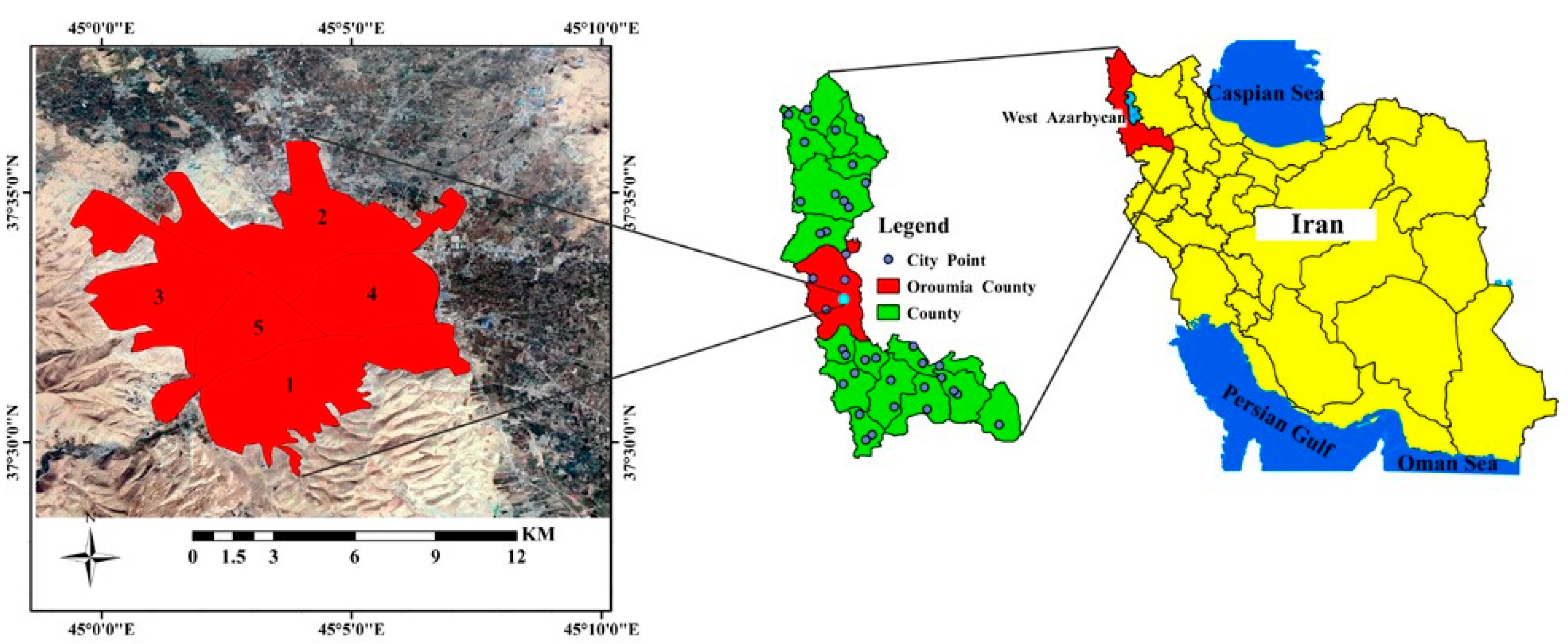
Figure 1. Location of the city of Urmia in Iran.
Sustainability 14 15625 g001
Figure 2. Research flowchart.
Sustainability 14 15625 g002
Figure 3. LULC maps (ac) for the study region in the three analyzed intervals 2000, 2010, and 2020 respectively.
Sustainability 14 15625 g003
Figure 4. The graphic shows the spatial change of the built-up, soil, vegetation, and rocky areas (ha) for the years 2000, 2010, and 2020.
Sustainability 14 15625 g004
Figure 5. Comparison of LULC map under the current state (upper maps) and LULC map produced by the classification method using the CA–Markov (lower-left map) and ANN (lower-right map) method.
Sustainability 14 15625 g005
Figure 6. LULC prediction map for 2030 ((a) CA–Markov (b) ANN) and the 2020–2030 changes ((c) change map by CA–Markov; (d) change map by ANN).
Sustainability 14 15625 g006
Figure 7. The diagram of LULC areas (ha) in 2030.
Sustainability 14 15625 g007
Table 1. Sample points size for classification.
Sample Point Size (Pixel)
YearBuild-UpRockySoilVegetation
2000251494115423564
2010296891313173098
20203311107212983012
Table 2. Classification results calculated for each year and class.
YearsAccuracy Assessment
Built-UpRockySoilVegetationAverageKappa Coefficient
200094.3696.1383.5999.7293.6391.49
201098.4896.8883.1899.7994.5892.48
202099.5199.4297.9199.5199.2198.94
Table 3. Evaluation of the role of the methods in simulating the LULCs. Blue numbers indicate the best results.
AlgorithmValidation MethodLULC
Built-UpRockySoilVegetationAverage
CA–MarkovCompleteness96.34%98.11%91.13%98.79%96.09%
Correctness97.36%91.77%98.28%98.47%96.47%
Quality93.99%89.89%94.63%96.16%93.67%
ANNCompleteness95.63%95.23%95.77%98.18%96.21%
Correctness98.06%95.31%96.29%95.62%96.32%
Quality93.85%92.11%94.79%94.44%93.8%
Publisher’s Note: MDPI stays neutral with regard to jurisdictional claims in published maps and institutional affiliations.