Hydrodynamics of the Instream Flow Environment of a Gravel-Bed River

Abstract

This work was aimed at comparing the instream flow environment of four basic hydromorphological units of a mountain gravel-bed river: pools, runs, riffles and rapids. A survey was performed during the average flow stage on the Skawa River in southern Poland. In the 3.5 km long reach, 31 physical habitats were surveyed: eight pools, eight runs, nine riffles and seven rapids. Using Micro ADV Sontek equipment, instantaneous velocity time series components were measured at eight locations in three positions—z/h = 0.2, 0.4 and 0.6—in each unit. Turbulence descriptors—the mean components of velocity, turbulence intensities calculated as the root mean square of velocity component time series, turbulent kinetic energy TKE, Reynolds shear stresses and standard hydraulic attribute, i.e., Froude number—were estimated. Although there was a wide dispersion of the turbulence variable distributions, a standard tendency of decreased mean velocity and increased turbulence towards the bottom was observed. Most turbulence parameters—streamwise velocity, turbulence intensities, TKE and streamwise-vertical Reynolds shear stresses—reveal differences of instream flow environment between the pools, runs and riffles. In addition, the mean turbulence intensities suggested a 1:2:3:3 proportion of turbulence intensity in pools, runs, riffles and rapids, respectively. Riffles and rapids, in general, have similar turbulence values, whereas rapids are deeper and visually more energetic.

1. Introduction

River morphology is one of the basic factors involved in determining instream flow environments concerning the aspect of hydraulics. Alluvial channels form a bed shape by sediment transport, especially during floods. The channel topography and hydrological regime create the habitat diversity for organisms that live in river ecosystems. Spatially distinct units can be used to describe the diversity of an instream flow environment. River channels can be divided into several morphological forms described in many classifications: geomorphic units, physical biotopes, physical habitats, hydraulic biotopes and mesohabitats. Although the definitions of these terms may differ to some degree, all refer to features that can be viewed as river hydromorphological units and used in the context of this work. A hydromorphological unit is a spatially distinct instream flow environment that is characterized by uniform hydraulic attributes created by the interactions between the discharge and the channel topography. In ecological terms, such units are viewed as the abiotic component of habitat [1]. Biologists often use the term “habitat” to describe the variability of a channel in terms of hydraulic conditions in which aquatic organisms exist [2]. The restoration of species diversity in an ecosystem requires morphological diversity in the river channel. Habitat diversity has been employed as a tool for assessing the current ecological status of rivers and the effectiveness of measures introduced to improve them [3,4]. The identification and parameterization of hydromorphological units is currently an important aspect in the management of water systems, as this allows for the prediction, evaluation and design of river habitats [5]. The parameters most commonly used in habitat identification include observations of the bottom topography, sediment and surface flow pattern. Water surface behavior reflects hydraulic conditions of a unit such as water velocity, depth or river bed grain size [5,6,7]. This approach is very useful because it can be employed by biologists, geomorphologists and engineers, who also have an interest in the ecological quality of river channels.

The study of hydraulic conditions in hydromorphological units has been focused on temporal and spatial averaging of velocity and depth. Several authors have pointed to the need to analyze the water flow in hydromorphological units related to the turbulent flow [1,8]. Water flow turbulence exhibits velocity pulsation, which directly and indirectly influences various ecological processes, including the development of the bottom flora [8], the distribution of food resources and the reactions of predators [9]. In addition, the amount of turbulence influences the life processes of fish: such as their energy consumption during movement [10,11] and the habitat they choose [12]. Studies conducted so far have indicated the legitimacy of undertaking work on the characteristics of turbulent motion in habitats [8]. Harvey and Clifford [1] posited that the parameters used for describing turbulent motion might be used to supplement existing classifications. Smith and Brannon [13] suggested that turbulence intensity might prove useful for the description of habitats because hydromorphological units often do not differ in terms of average parameters, but may differ in terms of turbulent motion parameters. The spatial distribution of turbulent flow properties around roughness elements has been previously described [14,15]. However, there is a theory that the effect of roughness on flow properties is local. At the scale of pools and riffles, spatial patterns of turbulence properties might be controlled by gross morphology rather than by individual boulders or pebble clusters [16,17]. Only a few studies have focused on the spatial distribution of turbulent flow properties at the scale of pools and riffles. To date, we still lack a detailed description of these morphological contexts.

In this article, we attempt to fill these gaps by delivering new insights into the hydraulics of the basic hydromorphological units of a gravel-bed river using detailed three-dimensional velocity structure and turbulence features. We address the hypothesis that there are differences between the hydraulic properties of four basic hydromorphological units: pools, runs, riffles and rapids. As an example of a natural gravel-bed channel, we chose a section of sub-mountain reach of the Skawa River in southern Poland.

2. Materials and Methods

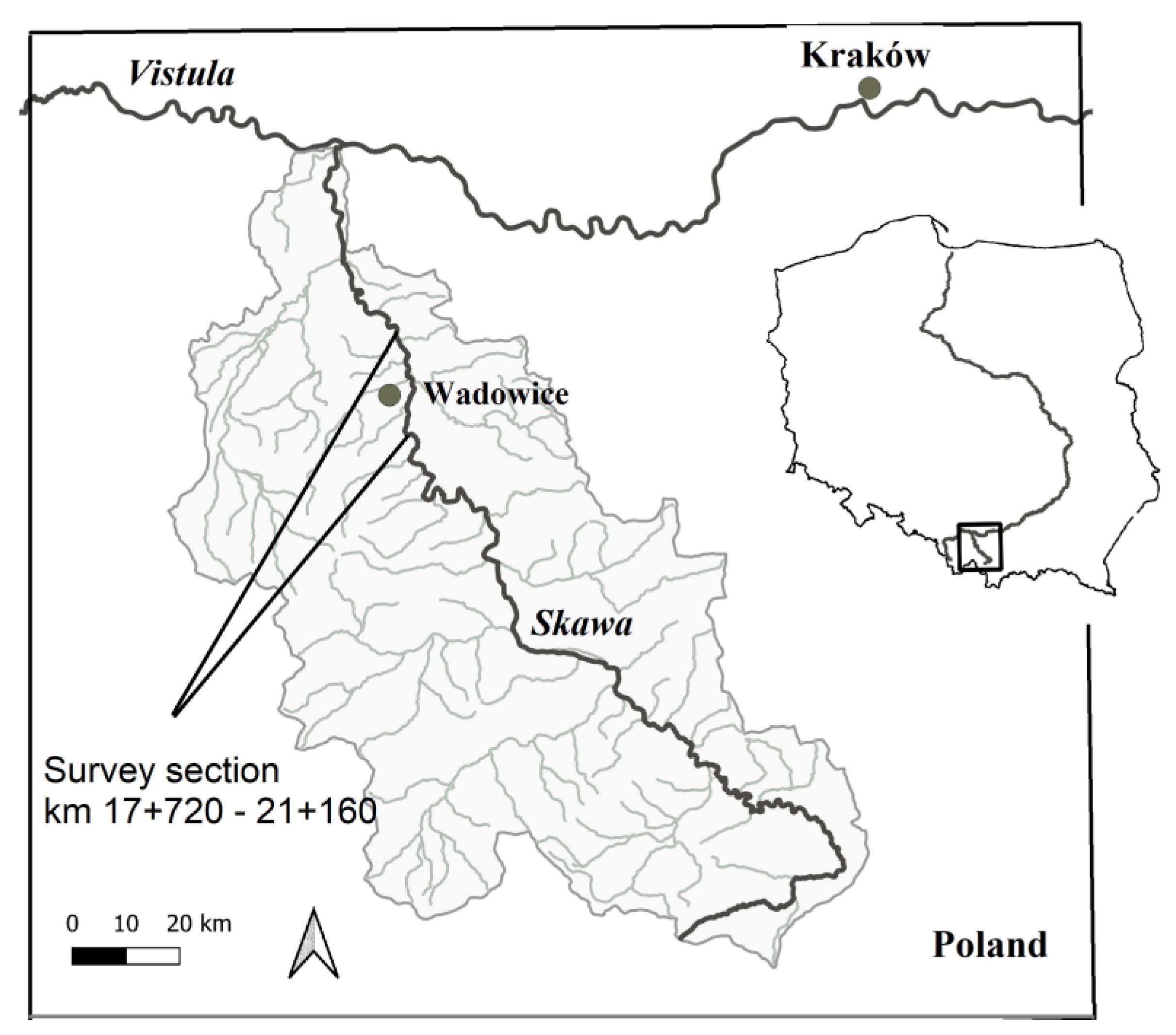
2.1. Study Site

Detailed velocity measurements were collected along a 3.5 km long reach of the Skawa River in southern Poland (Figure 1). The Skawa basin covers the central part of the High Beskids, the Central Beskids and the Lanckorona Foothills. The Skawa is a right tributary of the Vistula and is 95 km long with a catchment area of about 1180 km². Until recently, it was only the mountain river of this type without a dam reservoir; the fieldwork was completed before the dam was built.

We performed the survey on a 3.5 km long reach, located in the lower part of the river, where the catchment (area 833 km²) had a submontane character, the mean watercourse slope was 0.23%, the width of the water-filled channel was 20–30 m. The measurements were carried out under low stage conditions (discharge 3.5–5 m³·s⁻¹), while the mean annual flow was 12.75 m³·s⁻¹ and the mean low flow was 1.95 m³·s⁻¹.

2.2. Field Methods

Hydromorphological units were identified in the channel based on the hydraulics and morphology (local lateral and longitudinal channel topography). We distinguished these units based on observations of the water depth, velocity and surface flow type according to

Table 1. Description hydromorphological units modified after Bisson et al. [18] and Parasiewicz [19].

Hydromorphological Unit	Description
Pool	A channel segment with a concave longitudinal profile, high depth, slow water flow and smooth water surface Hydraulic summary: deep and slow flow
Run	A monotonous channel segment with a well-defined thalweg, moderate velocity and moderate depth, ripples or traveling waves on the water surface Hydraulic summary: medial depth and medial flow velocity
Riffle	A shallow area with fast current velocity and strong turbulence on the surface visible as standing unbroken or broken waves Hydraulic summary: shallow and fast flow
Rapid	A high gradient morphological form with very fast current velocity and turbulence on the water surface (standing waves), usually occurs downstream of a riffle Hydraulic summary: medial depth and fast flow

. Detailed measurements of three-dimensional velocity components are time-consuming, so we took the measurements under specifically different discharges within the range of the low flow for this section (using readings from the gauging station at Wadowice). Because we investigated the hydromorphological units, not only morphological units, the areas of the particular units changed with discharge change; borders between the units are migrating with time. Figure 2 presents examples of typical unit sequences in the channel. Our goal was to survey at least eight units of the same type: pools, runs, riffles and rapids. However, when measuring the riffles, we decided to collect data from nine units due to the reduced signal quality in a turbulent flow. After checking the data quality we found that the measurements from one rapid were not correct, so we rejected this unit. For analysis, we used 32 units: eight pools, eight runs, nine riffles and seven rapids; examples of unit mosaics are presented in Figure 2a,b.

We measured the velocity components and flow depths at eight locations in each individual unit (Figure 2c). The velocity measurements were taken using a MicroADV Sontek at three positions, z/h = 0.2, 0.4 and 0.6, where z is the height in the water column from the bottom and h is the local flow depth (Figure 3 and Figure 4). Because the boundary layer makes up to 30% of the water column [20], we chose the 0.2 h level as a representative of the near-bed hydraulics. We measured the velocity at the 0.4 h level following the assumption of the popular (in fluvial morphology) six-tenths method that the 0.4 h velocity most often coincides with the average velocity in a hydrometric profile [21,22]. It is difficult to assess the water velocity of the entire hydrometric profile in highly turbulent flows and therefore ecohydraulics investigations (in gravel bed) tend to use average velocity measured at 0.4 h above the bottom [23,24]. As a representative value for the maximum speed in the water column, we took the velocity at the 0.6 h level. The upper part of the velocity profile in a turbulent flow is the most difficult to measure using an acoustic probe. During the fieldwork efforts to do measurements in the rapids unit, we found that 0.6 h is the highest position at which we could obtain accurate measurements due to the excessive aeration of the flow caused by proximity to the surface. Time series of instantaneous velocity components (x-streamwise, y-transverse and z-vertical directions) were recorded for 60 s at a frequency of 20 Hz, as has been suggested [25]. The MicroADV probe was attached to an adjustable surveying tripod, allowing the probe to be stably positioned at any point in the river (Figure 3).

2.3. Calculations

At the start, we had 24 measurements in each from the 32 units, 768 time series in total. To ensure data accuracy in post-processing, a minimum signal-to-noise ratio SNR > 5 was applied and a correlation coefficient COR > 40%, which was acceptable for highly turbulent flows [26]. Outlier values were removed with the phase-space threshold despiking method [27,28]. At the end of the post-processing, time series with less than 1000 of the individual data were automatically excluded from further analysis. After post-processing, we had 753 time series to analyze (

Table 2. Number of time series in each hydromorphological unit type at three measurement positions.

Sampling Position	Pools	Runs	Riffles	Rapids
0.2 h	64	63	67	56
0.4 h	64	63	71	55
0.6 h	64	63	70	53

).

Each velocity measurement was separated into mean and fluctuating components:

u = U + u′

(1)

where u is the instantaneous streamwise velocity, U is the mean streamwise velocity for a time series and u′ is the fluctuating component of the instantaneous velocity. Transverse and vertical velocities were similarly, respectively, decomposed as v = V + v′ and w = W + w′.

The mean velocity components (U, V, W) were used to calculate the magnitude of the three-dimensional velocity vector (Muvw) for each time series:

Muvw = (U² + V² + W²)^0.5

(2)

Turbulence intensities that reflect velocity fluctuations were calculated as the root mean squares of the streamwise, transverse and vertical velocities (RMSu, RMSv, RMSw) for each time series.

Moreover, to represent the overall, three-dimensional turbulence intensity, the average turbulent kinetic energy (TKE) was calculated for each time series:

TKE = 0.5 (RMSu² + RMSv² + RMSw²)

(3)

We also included a contribution to the turbulent energy of streamwise (TKEu), transverse (TKEv) and vertical (TKEw) velocity pulsation.

Another important turbulence feature, albeit rarely reported in ecohydraulics experiments, is the Reynolds stresses representing the turbulent flux of momentum [29]. We included the vertical and horizontal Reynolds shear stresses τ_xz and τ_xy, respectively. The vertical Reynolds stresses were calculated using the covariance of the streamwise and vertical velocity components:

$${\mathsf{\tau }}_{\mathrm{x}\mathrm{z}}=-\varrho \overline{\left( {\mathrm{u}}^{\prime } {\mathrm{w}}^{\prime }\right)}, {\mathsf{\tau }}_{\mathrm{x}\mathrm{y}}=-\varrho \overline{\left( {\mathrm{u}}^{\prime } {\mathrm{v}}^{\prime }\right)},$$

(4)

where ρ is water density.

We also considered the standard hydraulic variable, the Froude number (Fr) calculated for each water column using the magnitude velocity at 0.4 h.

Fr = Muvw/(g·d)

(5)

where Muvw is the magnitude of the three-dimensional velocity at position z/h = 0.4 (m·s⁻¹), g is the acceleration due to gravity (m·s⁻²) and d is the water depth (m).

Our investigation was undertaken in order to compare the hydraulic features of hydromorphological units, so we collected all our measurements from eight pools as a representation of the pool unit type. Therefore, the mean values of all the variables for statistical comparison were calculated from around 60 measurements (Table 2). The variables for each unit type were tested for normality using the Kolmogorov–Smirnov test. We also checked the homogeneity of variance with Levene’s test. Because there was no equality in the variances in the groups, we decided to study the differences among the unit types using the Kruskal–Wallis test (insignificant difference between variables at the 0.05 level). All statistical calculations were performed using Statistica 12 software.

3. Results

The measured flow depth values ranged from 35.8 cm in the riffles to 85.1 cm in the pools in all unit types, while the runs and rapids had similar depths of 53.2 cm. A comparison of magnitude velocity between the different units revealed differences between the pools, runs and riffles at all three depths, but no differences were found between the riffles and rapids. The riffles and rapids were characterized by higher velocity values than the pools and runs. The mean velocity for the runs was higher than for the pools at every depth. Generally, the velocity increased from 0.2 h to 0.6 h depth (

Table 3. Spatially averaged flow depth and magnitude velocity for each hydromorphological unit showing the mean value (standard deviation) and results from the statistical comparison between units (cm).

Variable	Sampling Position	Pools	Runs	Riffles	Rapids
Depth (cm)		85.1 (54) a1	53.2 (32) b	35.8 (20) c	53.2 (38) b
Magnitude velocity Muvw (cm2·s−1)	0.2 h	38.2 (3.4) a	64.4 (27.1) b	79.3 (27.6) c	87.8 (36.5) c
	0.4 h	45.6 (5.4) a	81.7 (34.3) b	106.6 (54.5) c	115.1 (63.9) c
	0.6 h	49.2 (8.5) a	91.9 (38.2) b	121.6 (65.3) c	131.4 (78.9) c

Note ¹ Different letters (^a, ^b, ^c) represent significant differences among the hydromorphological units at p = 0.05 using the Kruskal–Wallis H test.

).

The statistical analysis of the spatially averaged streamwise velocity U and pulsation components RMSu, RMSv and RMSw at 0.2 h identified three significantly different hydraulic groups—pools, runs and riffles—with no discrimination between riffles and rapids (Figure 5a,d–f). The stream flow velocity ranged from 38 cm·s⁻¹ in the pools to 80 and 88 cm·s⁻¹ in the riffles and rapids, respectively. The transverse velocities V had similar values in both cross-stream directions, so the mean value was close to zero (Figure 5b). Only vertical velocity shows discrimination between the riffles and rapids, where more rapids values had a surface direction than a bottom direction compared with the riffles (Figure 5c). Overall, the dispersal of turbulence variables followed the order pools < runs < riffles ≈ rapids. The streamwise turbulence intensity RMSu was the highest and ranged from 7 cm·s⁻¹ in the pools and 13 cm·s⁻¹ in the runs to 20 cm·s⁻¹ in the riffles and rapids. In the rapids, the streamwise pulsation is more clustered around the mean than in the riffles and runs; the standard deviation of the RMSu value in the rapids was 3 cm·s⁻¹, while in the riffles, it was nearly 5 cm·s⁻¹ (Figure 5d). The horizontal turbulence intensity RMSv was lower, from 5 cm·s⁻¹ in the pools, 10 cm·s⁻¹ in the runs to 15 cm·s⁻¹ in the riffles and rapids (Figure 5e). The vertical pulsation RMSw were the lowest, ranging from 4 cm·s⁻¹ in the pools, 8 cm·s⁻¹ in the runs to 11 cm²·s⁻¹ in the pools and riffles (Figure 5f). The distribution of turbulence variables at the 0.4 h position was similar to those of the near bottom zone. The streamwise velocity at 0.4 h was higher than at near bed, ranging from 44 and 80 cm·s⁻¹ in the pools and runs, to 103 and 112 cm·s⁻¹ in the riffles and rapids, respectively (Figure 6a). The velocity pulsation at 0.4 was slightly lower than at 0.2 h. The turbulence intensity in the stream direction ranged from 6 cm²·s⁻¹ in the pools and 11 cm·s⁻¹ in the runs to 19 cm·s⁻¹ in the riffles and rapids (Figure 6d). The horizontal pulsations RMSv ranged from 5 cm·s⁻¹ in the pools, within 9 cm·s⁻¹ in the runs to 13 cm·s⁻¹ in the riffles and rapids (Figure 6e). The vertical pulsations RMSw were the lowest, ranging from 3 cm²·s⁻¹ in the pools, to 6 cm·s⁻¹ in the runs and 9 cm·s⁻¹ in the riffles and rapids (Figure 6f). A similar hydraulic pattern was recorded at 0.6 h apart from vertical velocity, where there was no distinction between the riffles and the rapids (Figure 7c). On average, the velocity values at 0.6 h were higher than at 0.4 h (Figure 5a), whereas the turbulence intensities were lower. The streamwise pulsation ranged from 5 cm·s⁻¹ in the pools, to 11 cm²·s⁻¹ in the runs and 16 cm·s⁻¹ in the riffles and rapids (Figure 7d). The horizontal pulsation RMSv ranged from 4 cm·s⁻¹ in the pools to 8 cm·s⁻¹ in the runs and 12 cm·s⁻¹ in the riffles and rapids (Figure 7e). The vertical pulsations RMSw had the same mean values at 0.4 h and 0.6 h (Figure 7f).

Turbulent kinetic energy TKE allowed discrimination between three basic hydromorphological units: pools, runs and riffles, with rapids being merged with riffles, irrespective of depth. Generally, the TKE rises in the bottom direction. The pools had spatially averaged TKE mean values of 49, 41 and 32 cm²·s⁻¹ at 0.2 h, 0.4 h and 0.6 h, respectively. In the runs, the TKE ranged from 115 cm²·s⁻¹ at 0.6 h to 180 cm²·s⁻¹ at 0.2 h. On average, the riffles and rapids had the highest TKE values from 270 and 257 cm²·s⁻¹ at 0.6 h position to 391 and 394 cm²·s⁻¹ at 0.2 h, respectively (Figure 8). The contribution to the turbulent kinetic energy of the velocity pulsations is provided in

Table 4. Contribution to the turbulent energy of streamwise (TKE_u), transverse (TKE_v) and vertical (TKE_w) velocity pulsations (%) with the means (standard deviation) for each hydromorphological unit types.

TKE Component	Sampling Position	Pools	Runs	Riffles	Rapids
TKE_u		51 (35)	53 (34)	54 (40)	54 (26)
TKE_v	0.2 h	32 (18)	30 (22)	30 (22)	30 (21)
TKE_w		17 (9)	17 (12)	16 (11)	16 (11)
TKE_u		51 (32)	52 (43)	54 (35)	54 (41)
TKE_v	0.4 h	32 (20)	30 (23)	30 (22)	29 (19)
TKE_w		17 (10)	18 (13)	16 (11)	17 (11)
TKE_u		48 (34)	52 (40)	55 (43)	53 (41)
TKE_v	0.6 h	33 (18)	30 (23)	29 (22)	30 (21)
TKE_w		18 (9)	18 (13)	16 (10)	17 (12)

. The streamwise component contributed 48–55%, with transverse and vertical components making up 29–33% and 16–18%, respectively, from all positions in all unit types.

The vertical Reynolds stresses distinguished three different hydraulic groups at every depth. Riffles were merged with rapids. The value of τ_xz in every unit increased in the bottom direction. In the pools, τ_xz was the lowest, with 0.48 N·m⁻² at 0.6 h, to 0.8 N·m⁻² at 0.4 h and 1.19 N·m⁻² at 0.2 h. The runs had τ_xz values four times higher than the pools, from 2.4 N·m⁻² at 0.6 h to 4.9 N·m⁻² at 0.2 h. The Riffles and rapids were characterized by the highest τ_xz values, with, respectively, 5.1 and 4.8 N·m⁻² at the 0.6 h position to 10.5 and 11.1 N·m⁻² at 0.2 h depth (Figure 9d–f). The transverse Reynolds stresses τ_xy did not reveal any differences between the units because the values were also positive and negative, so the magnitudes were around zero. Spatial heterogeneity, as expected, increased in the order pools < runs < riffles ≈ rapids (Figure 9a–c). The Froude number distinguished three significantly different groups of hydraulic values, but did not discriminate between riffles and rapids. The spatially averaged Fr values ranged from 0.16 in the pools, to 0.37 in the runs and 0.51 and 0.57 in the rapids and riffles, respectively, (Figure 10).

4. Discussion

In this work, we acquired natural stream turbulent flow field data. The results can be used to improve our understanding of the influence of velocity fluctuation on relevant ecological processes. Research of Enders et al. [10] revealed that under naturally turbulent conditions, fish (Atlantic Salmon Parr) displayed high individual variability in their habitat use. Such heterogeneous use of habitat suggests that individuals are not constrained to a single habitat type but need each of them. Furthermore, no differences were observed in habitat use among the four daily periods (dawn, day, dusk and night) for individual parr.

Our results indicate that most turbulence parameters can be used to distinguish between different hydraulic environments in three basic hydromorphological units: pools, runs and riffles. Although riffles and rapids are substantially different hydraulic environments in the field, most turbulence variables did not exhibit this distinction. Only the vertical velocity distribution indicated a difference between riffles and rapids, showing that rapids had more bottom direction movement than riffles, which disappears at 0.6 h. Internal variability in the hydraulic values of riffles and rapids meant we could not identify any evident differences in their hydraulics.

Our results confirm the traditional velocity profile of a gravel-bed river with values decreasing in the bottom direction. In this study, we do not see the all separated profiles, only spatially averaged variables. However, research on cobble bed rivers has suggested that field data poorly reflect the logarithmic profile of velocity [30]. Finer sediment such as gravel is expected to have no influence over the entire velocity profile. As expected, the average magnitude velocity values Muvw were similar to the streamwise velocity component U in all units. We also observed a strong spatial variation in velocity with all units. The standard deviations of streamwise velocity components U are high in all units. Concerning depths and velocities, riffle is a good environment for spawning of Vimba vimba, Barbus peloponesius and Chondrostoma nasus [31].

The turbulence intensities RMSu, RMSv and RMSw distinguished three hydromorphological units, pools, runs and riffles. A gradation in the magnitudes of RMSu, RMSv and RMSw values interestingly had a proportions 1:2:3:3 between the pools, runs, riffles and rapids, respectively. This finding needs to be confirmed in a further study. Other studies have reported large RMSu variations in pool units (2–15 cm·s⁻¹) with rather simple distributions in riffles (2–3 cm·s⁻¹) [30,32]. Abel et al. [33] did not find any differences between glides and runs in terms of their RMSu, RMSv and RMw, but we did not use a glide unit as a separate unit from a run. Turbulence intensities RMSu, RMSv and RMSw increasing towards the bottom (in all units) are common phenomena in mountain rivers [33]. This is caused by the influence of bottom roughness on the reduction in average velocity and, at the same time, the increase in turbulence intensity. This tendency was previously reported in a study on the turbulent flow structure on a gravel-bed river, with velocities ranging from 0.3 to 0.7 cm·s⁻¹ and turbulence intensity ranging from 5 to 10 cm·s⁻¹ [14]. A similar distribution in turbulence intensity has been reported from a river with a sandy bottom with velocities of 0.1 m·s⁻¹ at 1 m depth [34]. Thus, it can be concluded that in the near bed zone, the velocity is characterized by lower average values and large pulsations. In the aspect of ecology, for invertebrates, even if there is near bed streamwise velocity influence assemblage composition and the number of taxa is at its highest, the transverse turbulence is equal to or of greater importance than turbulence in the downstream direction [35].

The turbulent kinetic energy displayed similar patterns to those revealed by the individual RMS components and also distinguished three different hydraulic patches in the order: pools > runs > riffles ≈ rapids. We expected to find rapids with higher TKE values; our findings could not confirm this hypothesis. Wilcox and Wohl [24] interestingly reported higher TKE values in a pool rather than a run unit. However, other studies have confirmed higher TKE in riffles than in pools [9,12,36]; our findings are compatible with these. The TKE increases towards the bottom because the roughness of the bed material causes the velocity pulsation to increase by up to several hundred percent compared to a smooth bottom [37]. This tendency has also been identified in studies on a sandy river with similar depths to those of the Skawa [34]. Our TKE value was increasing at a depth of 0.2 h, confirming the findings of an earlier study [38].

Regarding the velocity component contributions to the TKE, our study has confirmed Sukhodov et al.’s [20] findings that the streamwise component is responsible for 45–55% of the TKE, irrespective of flow depth. Our study suggests it is 51–55%. They also found that the remaining contributions from the transverse and vertical components vary with depth, with the vertical component being lowest near the bed and the surface and mid-profile contributions to TKE averaging approximately 30% and 20% from the transverse and vertical components, respectively [20]. Our observation assumed similar contributions of about 29–32% and 16–18% from the transverse and vertical velocities, respectively, but we did not observe any variation within the water column. Wilcox and Wohl [24] also did not find variations within the water column, but they depict that contributions from streamwise velocities are smaller (by an average of 36%), whereas turbulence in the vertical velocity component contributes approximately half of the TKE.

The horizontal Reynolds shear stress is the most important Reynold shear stress component in the aspect of the affection on species movements but it is rarely reported in ecohydraulics research [29,39]. Our τ_xy values were not so high as Silva et al. [39] reported as high turbulence areas in a fishway (τxy 20–60 N·m⁻²), which are avoided by fish—Iberian Barber. Concerning hydromorphological units, we once again can only observe the strong heterogeneity of riffles and rapids. Other studies have also assumed that Reynolds stresses are similar in hydromorphological units [30,32]. Abel et al. [32] reported the same distribution of τ_xy in glides and runs as we observed in pools but they had different distributions for τxz, which also are similar in glides and runs and varied around zero. Our study reveals that τ_xz is greater than zero, which means that net flux of turbulent momentum is generally positive for all units in agreement with the theory suggesting that turbulence is exported from the bed towards the surface, as was reported also in Wilkes [36]. Moreover, τ_xz had different distributions in the pools, runs and riffles and again increased towards the bottom within the water column.

In a gravel-bed river with a slope exceeding 1%, Mosley [40] reported smaller Froude numbers for the investigated units. Allen’s classification provides a Froude number below 0.15 for pools and above 0.25 for riffles [41]. Kemp et. al. [42] suggest that valuable biology factors are connected with Fr, ex. moss occurs within 0.3–0.4 and macroalgae 0.3–0.55. Some authors have suggested that the Froude number was not a good enough parameter to be used to distinguish between habitats [5,43]. However, our results have demonstrated that the Froude number differed for three basic habitats: pools 0.16 < runs 0.37 < riffles 0.57 ≈ rapids 0.51. Interestingly, in the field, we observed rapids as being more energetic units than the riffles. However, we may obtain similar Froude numbers for different depth–velocity combinations; in rapids, high velocity is divided by great depth, so this parameter may overlook important unit features.

Our research reveals the heterogeneity of the instream flow environment even if we characterized it using hydromorphological units. In the analysis of turbulence properties, a large dispersion of local values is observed, which indicates difficulties with an unambiguous determination of the amount of turbulence in individual units. Our findings may be considered during the design of future ecohydraulics models.

5. Conclusions

Our results revealed that most turbulence parameters indicate different hydraulic environments in terms of three basic hydromorphological units: pool, run and riffle. Although riffles and rapids are substantially different hydraulic environments in the field, most turbulence variables did not highlight this difference. The turbulence components suggest a proportion of turbulence intensity 1:2:3:3 in pools, runs, riffles and rapids, respectively. Although there was a wide dispersion in the distribution of the turbulence variables, the standard tendency of a decreased mean velocity and increased turbulence towards the bottom was observed. Hydromorphological units present very strong spatial variability, so their magnitudes should be interpreted in terms of this understanding.

References

1. Harvey, G.; Clifford, N. Microscale Hydrodynamics and Coherent Flow Structures in Rivers: Implications for the Characterization of Physical Habitat. River Res. Appl. 2009, 180, 160–180. [Google Scholar] [CrossRef]
2. Kownacki, A.; Soszka, H. Wytyczne do Oceny Stanu Rzek na Podstawie Makrobezkręgowców Oraz do Pobierania Prób Makrobezkręgowców w Jeziorach; IOŚ: Warszawa, Poland, 2004. [Google Scholar]
3. Mouton, A.M.; Schneider, M.; Depestele, J.; Goethals, P.L.M.; De Pauw, N. Fish Habitat Modelling as a Tool for River Management. Ecol. Eng. 2007, 29, 305–315. [Google Scholar] [CrossRef]
4. Książek, L.; Bartnik, W. Wykorzystanie warunków hydraulicznych do oceny typów siedlisk w korycie rzecznym. Nauk. Przyr. Technol. 2009, 3, 89. [Google Scholar]
5. Clifford, N.J.; Harmar, O.P.; Harvey, G.; Petts, G.E. Physical Habitat, Eco-Hydraulics and River Design: A Review and Re-Evaluation of Some Popular Concepts and Methods. Aquat. Conserv. Mar. Freshw. Ecosyst. 2006, 16, 389–408. [Google Scholar] [CrossRef]
6. Harper, D.; Everard, M. Why Should the Habitat—Level Approach Underpin Holistic River Survey and Management? Aquat. Conserv. Mar. Freshw. Ecosyst. 1998, 8, 395–413. [Google Scholar] [CrossRef]
7. Jowett, I.G. A Method for Objectively Identifying Pool, Run, and Riffle Habitats from Physical Measurements. N. Z. J. Mar. Freshw. Res. 1993, 27, 241–248. [Google Scholar] [CrossRef]
8. Cardinale, B.; Palmer, M.; Swan, C. The Influence of Substrate Heterogeneity on Biofilm Metabolism in a Stream Ecosystem. Ecology 2002, 83, 412–422. [Google Scholar] [CrossRef]
9. Roy, M.; Roy, A.; Legendre, P. The Relations between “standard” Fluvial Habitat Variables and Turbulent Flow at Multiple Scales in Morphological Units of a Gravel-bed River. River Res. Appl. 2010, 26, 439–455. [Google Scholar] [CrossRef]
10. Enders, E.C.; Roy, M.L.; Ovidio, M.; Hallot, É.J. Habitat Choice by Atlantic Salmon Parr in Relation to Turbulence at a Reach Scale. N. Am. J. Fish. Manag. 2009, 29, 1819–1830. [Google Scholar] [CrossRef] [Green Version]
11. Lupandin, A.I. Effect of Flow Turbulence on Swimming Speed of Fish. Izv. Akad. Nauk Ser. Biol. 2005, 32, 558–565. [Google Scholar] [CrossRef]
12. Smith, D.L.; Brannon, E.L.; Odeh, M. Response of Juvenile Rainbow Trout to Turbulence Produced by Prismatoidal Shapes. Trans. Am. Fish. Soc. 2005, 134, 741–753. [Google Scholar] [CrossRef]
13. Smith, D.L.; Brannon, E.L. Influence of Cover on Mean Column Hydraulic Characteristics in Small Pool Riffle Morphology Streams. River Res. Appl. 2007, 23, 125–139. [Google Scholar] [CrossRef]
14. Roy, A.G.; Buffin-Blanger, T.; Lamarre, H.; Kirkbride, A.D. Size, Shape and Dynamics of Large-Scale Turbulent Flow Structures in a Gravel-Bed River. J. Fluid Mech. 2004, 500, 1–27. [Google Scholar] [CrossRef] [Green Version]
15. Tritico, H.M.; Hotchkiss, R.H. Unobstructed and Obstructed Turbulent Flow in Gravel Bed Rivers. J. Hydraul. Eng. 2005, 131, 635–645. [Google Scholar] [CrossRef]
16. Lamarre, H.; Roy, A.G. Reach Scale Variability of Turbulent Flow Characteristics in a Gravel-Bed River. Geomorphology 2005, 68, 95–113. [Google Scholar] [CrossRef]
17. Legleiter, C.J.; Phelps, T.L.; Wohl, E.E. Geostatistical Analysis of the Effects of Stage and Roughness on Reach-Scale Spatial Patterns of Velocity and Turbulence Intensity. Geomorphology 2007, 83, 322–345. [Google Scholar] [CrossRef] [Green Version]
18. Bisson, P.; Montgomery, D.; Buffington, J. Valley segments, stream reaches, and channel units. In Methods in Stream Ecology; Richard, H., Gary, L., Eds.; Elsevier: London, UK, 1996; pp. 23–50. [Google Scholar]
19. Parasiewicz, P. The MesoHABSIM Model Revisited. River Res. Appl. 2007, 23, 893–903. [Google Scholar] [CrossRef]
20. Sukhodolov, A.; Thiele, M.; Bungartz, H. Turbulence Structure in a River Reach with Sand Bed. Water Resour. Res. 1998, 34, 1317–1334. [Google Scholar] [CrossRef]
21. Holmes, R.R. Surface water data collection. In Field Methods for Hydrologic and Environmental Studies; Harris, M., Ed.; US Geological Survey: Urbana, IL, USA, 2001; pp. 1–77. [Google Scholar]
22. Kinzel, P.J.; Wright, C.W.; Nelson, J.M.; Burman, A.R. Evaluation of an Experimental LiDAR for Surveying a Shallow, Braided, Sand-Bedded River. J. Hydraul. Eng. 2007, 133, 838–842. [Google Scholar] [CrossRef] [Green Version]
23. David, G.C.L.; Legleiter, C.J.; Wohl, E.; Yochum, S.E. Characterizing Spatial Variability in Velocity and Turbulence Intensity Using 3-D Acoustic Doppler Velocimeter Data in a Plane-Bed Reach of East St. Louis Creek, Colorado, USA. Geomorphology 2013, 183, 28–44. [Google Scholar] [CrossRef]
24. Wilcox, A.C.; Wohl, E.E. Field Measurements of Three-Dimensional Hydraulics in a Step-Pool Channel. Geomorphology 2007, 83, 215–231. [Google Scholar] [CrossRef]
25. Buffin-Bélanger, T.; Roy, A.G. 1 Min in the Life of a River: Selecting the Optimal Record Length for the Measurement of Turbulence in Fluvial Boundary Layers. Geomorphology 2005, 68, 77–94. [Google Scholar] [CrossRef]
26. Martin, V.; Fisher, T.; Millar, R.; Quick, M. ADV Data analysis for turbulent flows: Low correlation problem (ASCE). In Hydraulic Measurements and Experimental Methods 2002; Wahl, T.L., Pugh, C.A., Oberg, K.A., Vermeyen, T.B., Eds.; American Society of Civil Engineers: Estes Park, CO, USA, 2002; pp. 1–10. [Google Scholar]
27. Goring, D.; Nikora, V. Despiking Acoustic Doppler Velocimeter Data. J. Hydraul. Eng. 2002, 128, 117–126. [Google Scholar] [CrossRef] [Green Version]
28. Wahl, T.L. Discussion of “Despiking Acoustic Doppler Velocimeter Data” by Derek, G. Goring and Vladimir, I. Nikora. J. Hydraul. Eng. 2002, 128, 484–488. [Google Scholar] [CrossRef] [Green Version]
29. Trinci, G.; Harvey, G.L.; Henshaw, A.J.; Bertoldi, W.; Hölker, F. Life in Turbulent Flows: Interactions between Hydrodynamics and Aquatic Organisms in Rivers. Wiley Interdiscip. Rev. Water 2017, 4, e1213. [Google Scholar] [CrossRef]
30. Stone, M.C.; Hotchikiss, R.H. Turbulence Descriptions in Two Cobble-Bed River Reaches. J. Hydraul. Eng. 2007, 133, 1367–1378. [Google Scholar] [CrossRef] [Green Version]
31. Brylińska, M. Ryby Słodkowodne Polski; Wydawnictwo Naukowe PWN: Warszawa, Poland, 1991. [Google Scholar]
32. Abel, S.; Hopkinson, C.; Hession, W. Hydraulic and Physical Structure of Runs and Glides Following Stream Restoration. River Res. Appl. 2016, 32, 1890–1901. [Google Scholar] [CrossRef]
33. Tritico, H.M. The Effects of Turbulence on Habitat Selection and Swimming Kinematics of Fishes. Ph.D. Thesis, University of Michigan, Ann Arbor, MI, USA, 2009. [Google Scholar]
34. Nikora, V.; Green, M.O.; Thrush, S.F.; Hume, T.M.; Goring, D. Structure of the Internal Boundary Layer over a Patch of Pinnid Bivalves (Atrina Zelandica) in an Estuary. J. Mar. Res. 2002, 60, 121–150. [Google Scholar] [CrossRef]
35. Reid, M.A.; Thoms, M.C. Surface Flow Types, near-Bed Hydraulics and the Distribution of Stream Macroinvertebrates. Biogeosciences 2008, 5, 1043–1055. [Google Scholar] [CrossRef] [Green Version]
36. Wilkes, M.A.; Maddock, I.A.N.; Acreman, M.C. A Hydrodynamic classification of mesohabitats. In Proceedings of the 10th International Symposium on Ecohydraulics, Trondheim, Norway, 21–27 June 2014. [Google Scholar] [CrossRef]
37. Nikora, V.; Aberle, J.; Biggs, B. Effects of Fish Size, Time to Fatigue and Turbulence on Swimming Performance: A Case Study of Galaxias Maculatus. J. Fish Biol. 2003, 63, 1365–1382. [Google Scholar] [CrossRef]
38. Nikora, V.I.; Goring, D.G.; Biggs, B.J.F. On Stream Periphyton-Turbulence Interactions. N. Z. J. Mar. Freshw. Res. 1997, 31, 435–448. [Google Scholar] [CrossRef]
39. Silva, A.T.; Santos, J.M.; Ferreira, M.T.; Pinheiro, A.N.; Katopodis, C. Effects of Water Velocity and Turbulence on the Behaviour of Iberian Barbel (Luciobarbus bocagei, Steindachner 1864) in an experimental pool-type fishway. River Res. Appl. 2011, 27, 360–373. [Google Scholar] [CrossRef]
40. Mosley, M. A Procedure for characterising river channels. In Water and Soil Miscellaneous Publication; Ministry of Works and Development: Wellington, New Zealand, 1982; Volume 32, p. 90. [Google Scholar]
41. Allen, K.R. The Horokiwi Stream: A Study of Trout Population. Fish. Bull. 1951, 10, 231. [Google Scholar]
42. Kemp, J.L.; Harper, D.M.; Crosa, G.A. The Habitat-Scale Ecohydraulics of Rivers. Ecol. Eng. 2000, 16, 17–29. [Google Scholar] [CrossRef]
43. Moir, H.J.; Pasternack, G.B. Relationships between Mesoscale Morphological Units, Stream Hydraulics and Chinook Salmon (Oncorhynchus Tshawytscha) Spawning Habitat on the Lower Yuba River, California. Geomorphology 2008, 100, 527–548. [Google Scholar] [CrossRef]
Figure 1. Location of the study site in southern Poland.
Sustainability 14 15330 g001
Figure 2. Examples of (a,b) hydromorphological unit mosaic in the channel and (c) arrangement of field measurements of depth and velocity for each unit.
Sustainability 14 15330 g002
Figure 3. ADV Sontek; the measurements with an example of time series sampling. An ADV Sontek taking measurements, connected to a computer by a cable.
Sustainability 14 15330 g003
Figure 4. Examples of hydrometric profiles—single locations of some hydromorphological units (streamwise U, transverse V and vertical W components); averages of at least a thousand individual values.
Sustainability 14 15330 g004
Figure 5. Distribution of turbulence variables at sampling position z/h = 0.2; Time averaged velocities (a) streamwise (U) (b) horizontal cross-stream (V) and (c) vertical (W) and pulsation in three directions given as the root mean square (d) RMSu, (e) RMSv, (f) RMSw by hydromorphological unit types; letters (a, b, c) indicate a significant difference between hydromorphological unit types (mean: line, standard deviation: box, min-max: whisker).
Sustainability 14 15330 g005
Figure 6. Distribution of turbulence variables at sampling position z/h = 0.4; Time averaged (a) streamwise (U) (b) horizontal cross-stream (V) and (c) vertical (W) and pulsation in three directions given as root mean square (d) RMSu, (e) RMSv, (f) RMSw by hydromorphological unit types; letters (a, b, c) indicate a significant difference between hydromorphological units (mean: line, standard deviation: box, min-max: whisker).
Sustainability 14 15330 g006
Figure 7. Distribution of turbulence variables at sampling position z/h = 0.6 h; Time averaged velocities (a) streamwise (U) (b) horizontal cross-stream (V) and (c) vertical (W) and pulsation in three directions given as root mean square (d) RMSu, (e) RMSv, (f) RMSw by hydromorphological units; letters (a, b, c) indicate a significant difference between hydromorphological units (mean: line, standard deviation: box, min-max: whisker).
Sustainability 14 15330 g007
Figure 8. Distribution of turbulent kinetic energy (TKE) in the hydromorphological units at sampling positions (a) 0.2 h, (b) 0.4 h, (c) 0.6 h, by hydromorphological unit types; letters (a, b, c) indicate a significant difference between hydromorphological units (mean: line, standard deviation: box, min-max: whisker).
Sustainability 14 15330 g008
Figure 9. Distribution of the vertical Reynolds stresses τxz in the hydromorphological units at sampling positions (a) 0.2 h, (b) 0.4 h, (c) 0.6 h and the horizontal Reynolds stresses τxy at (d) 0.2 h, (e) 0.4 h and (f) 0.6 h by hydromorphological unit types; letters (a, b, c) indicate a significant difference between units (mean: line, standard deviation: box, min-max: whisker).
Sustainability 14 15330 g009
Figure 10. Distribution of Froude number Fr units compared among the hydromorphological unit types; letters (a, b, c) indicate a significant difference between hydromorphological unit types (mean: line, standard deviation: box, min-max: whisker).
Sustainability 14 15330 g010