Sustainability Indicators of Groundwater Withdrawal in a Heavily Stressed System: The Case of the Acque Albule Basin (Rome, Italy)

Abstract

Groundwater sustainable yield is a concept widely treated theoretically in the literature. Moving from theoretical concepts to the definition of practical measures for groundwater management is not easy due to site-specific characteristics of the system. This study is aimed at identifying which factors influence the sustainable yield of the plain of Tivoli (Central Italy), where thermal springs with considerable flow (over 2 m³/s) emerge (or rather emerged) and supply a thermal plant. In the same plain, another profitable economic activity concerns the extraction of travertine; it caused a progressive decline in groundwater levels and in the discharge of the thermal springs. The hydrogeological history of the site and the data available in the literature and in new focused surveys are encapsulated in a simple flow model addressed to compare the pre- with the under-development conditions. The withdrawal of groundwater from the quarry area determined a significant impact on the water balance of the system. An increase in inflow from surrounding aquifers and a decrease in storage and in natural discharge of the travertine aquifer result in under-development conditions. Residual discharges towards the springs and river are very sensitive to the pumping flow rate of quarries, according to an inverse linear relationship; this hydrogeological feature may be adopted as an indicator of the sustainability of groundwater withdrawals from the plain. The residual discharge is most affected by the position of the pumping center in the groundwater flow net and its distance from boundaries to be captured, as well as on the depth and extent of the quarries. This lays the basis for developing sustainable management models of groundwater considering the economic and environmental aspects of the issue.

1. Introduction

The concept of groundwater sustainability has a long history and is today the subject of wide debate [1,2,3,4]. Starting from the concept of safe yield, in the literature, there are many definitions such as sustainable yield, sustainable groundwater development and sustainable groundwater management. Among these, a significant definition of groundwater sustainability is reported by Alley et al. [5], who define groundwater sustainability as the “development and use of ground-water in a manner that can be maintained for an indefinite time without causing unacceptable environmental, economic, or social consequences.” It follows that groundwater management based on the concept of sustainability calls for a multidisciplinary approach. The debated question is how to estimate sustainable yield. According to Pierce et al. [2], six factors influence the determination of sustainable yield, including: (i) recharge rates and storage conditions, (ii) water quality, (iii) discharge rates and environmental flows, (iv) legal constraints, (v) economic feasibility and (vi) issues of inter-generational equity. Only some of these components belong to the field of hydrogeology, which nevertheless is transversal and essential to coordinate a participatory and consensual agreement among the different stakeholders. Different views are found in the literature on the criteria leading to the definition of the sustainable yield of a system. Many approaches are based on the comparison of natural recharge and pumping rate, determining the safe yield as “the pumping rate that does not exceed the rate of natural recharge”. Others consider that the pumping rate only depends on the capture (i.e., the sum of the increase in recharge and decrease in discharge caused by pumping), which is independent from the natural recharge. Other approaches use the residual groundwater outflow from the system, which depends on natural recharge, and the development of the capture as criteria to define the sustainable yield [1,5,6,7,8,9,10,11,12,13,14,15].

The application of these criteria is not easy depending on the site-specific characteristics of the hydrogeological, environmental, economic, and social systems.

In the plain of Tivoli, located about 20 km east of Rome, important and well-known thermal springs, the Acque Albule, emerge (or rather emerged) and supply the thermal plant, Terme di Roma. In the same plain, another profitable economic activity concerns the extraction of travertine, practiced since Roman times. Until the 1970s, the flow of the Acque Albule springs had a flow rate of over 2 m³/s, outflowing on the surface from two lakes of karst origin (Regina and Colonnelle lakes). Since the 1970s, the extraction of travertine has involved increasing depths, until it reached the aquifer containing the thermal waters. It was then necessary to proceed to dewater the quarry area. This gave rise to a progressive decline in groundwater levels in the travertine aquifer and in the discharge of the Acque Albule springs. Several studies have been carried out on the hydrogeology of the Acque Albule Basin and on the impacts of dewatering (see references in the next section). The problem of the management of the plain’s groundwater still remains open, with the two economic activities (spa industry and mining) involving the same groundwater resources conflicting.

This study is aimed at identifying which factors influence the sustainable yield of the plain of Tivoli, where important groundwater resources in terms of quantity and quality are significantly exposed to pumping. The hydrogeological history of the site and the data available in the scientific literature, in technical reports and in new focused surveys are assimilated in a simple flow model specifically addressed to compare the pre-development with the under−development conditions.

2. Background Knowledge on Groundwater Flow and Anthropogenic Impacts in the Acque Albule Basin

The Tivoli Plain constitutes a morphological depression bordered to the north and to the east by the reliefs of the central Apennines, to the west by the gentle slopes of the Colli Albani volcanic complex and to the south by the Aniene River (Figure 1a).

The plain, with elevations between 40 and 80 m above sea level (asl), is a pull-apart subsiding basin (Acque Albule Basin) related to the movements of a strike-slip fault that is oriented N-S. The basin is filled with travertine (Lapis Tiburtinus) and alluvial, lacustrine, volcanic and marine Pliocene–Pleistocene deposits; travertine deposits are the most represented formation in the plain, covering an area of approximately 33 km², with a thickness from 10 to 90 m. The substrate of the Pliocene–Pleistocene deposits consists of a Mesozoic–Cenozoic carbonate succession of platform-to-basin environments. The fold-and-thrust carbonate successions outcrop in the reliefs bordering the plain [16,17]. In the plain, there are thermal springs, sinkholes and karst landforms located along the main faults [18,19,20].

From a hydrogeological point of view (Figure 1b), two overlapping aquifers are recognized in the plain: (i) a deep confined or leaky aquifer hosted in fractured Mesozoic–Cenozoic carbonate rocks (transmissivity of 10⁻¹ m²/s [21]), and (ii) a shallow unconfined to leaky aquifer within travertine deposits (transmissivity of 10⁻¹ m²/s [22]). The two aquifers are separated by an aquitard represented by low-permeability Pliocene–Pleistocene alluvial, lacustrine, volcanic and marine deposits. Flows from deep to shallow aquifer occur through the aquitard, especially through the fracture and fault zones of the carbonate bedrock and Pliocene deposits [21,22,23]. Studies performed at a regional scale have recognized a groundwater flow of about 4 m³/s, N-S oriented from carbonate reliefs towards the plain, discharging into the springs and the Aniene River [24,25]. An active groundwater circulation occurs in the travertine deposits recharged by meteoric infiltration in the plain, lateral inflow from carbonate reliefs and from the rises of the above-mentioned deep mineralized fluid from carbonate bedrock [26] (Figure 1a,b).

In the 1950s, several springs used to outflow in a doline field in the plain [30]; among them, the main group is represented by the Acque Albule springs (Figure 1a), characterized by mineralized waters (temperature of about 23 °C). The water from the springs (Acque Albule and other minor springs; Figure 1a), wells and the one drained from the quarries is of the Ca-HCO₃-SO₄ type (Figure 1c), characterized by total dissolved solid (TDS) values ranging from 0.8 to 2.4 g/L and dissolved inorganic carbon (DIC) from 7 to 16 mmol/kg, as defined in Carucci et al. [23]. This groundwater is the result of the mixing between the endmembers coming from the carbonate recharge areas and from the deeply buried Mesozoic–Cenozoic carbonate aquifer, enriched in CO₂ and other uprising fluids. The quality of the water emerging from the springs and drained from the quarries is very similar, as can be seen from the Schoeller-Berkaloff diagram (Figure 1c).

The spring regime and groundwater flow pattern in the Tivoli Plain have been conditioned over time by anthropogenic activities involving the historical travertine extraction and the exploitation for recreational purposes. A significant decrease in groundwater levels has been detected over time, up to some tens of meters in the quarry area. This is mainly due to the groundwater withdrawal necessary to extract travertine in dewatered conditions. The evolution of the groundwater levels from 1977 to 2009 is described in Del Bon et al. [31]. The lowering of the groundwater level reflected the flow rate of the springs and possibly also the groundwater flow rate discharging towards the Aniene River [28,32]. Until the 1970s, the Acque Albule springs had a flow rate of more than 2 m³/s, while since 2001, they reduced their natural outflow at the surface to zero. The pumping flow rate from the quarry area increased from about 1 m³/s in the 1970s to about 5 m³/s in 2008 [33].

Due to the complexity of the hydrogeological conceptual model, different numerical modeling approaches have been proposed to describe the impact of human activities on the travertine aquifer.

Brunetti et al. [34] examined the changes in the hydrogeological equilibrium of the Acque Albule Basin through a finite-element groundwater model. The authors considered a series of steady-state conditions representing the last 40 years, in order to verify the influences of groundwater withdrawals from the quarry area on the travertine aquifer. The calibration process was based on measured groundwater levels and flow rates, varying the hydraulic conductivity of the aquifer and maintaining the lateral recharge from the carbonate reliefs constant. The calibrated model was used to simulate a scenario in the pre-development conditions, before the activation of massive withdrawals from quarries. The authors point out that the dewatering has significantly modified the groundwater flow and the hydrogeological balance of the basin, assessing that a 30% reduction in water abstraction from the quarry area could restore the surface outflow of the Acque Albule springs [34].

A further model of the groundwater flow of the basin is proposed by La Vigna et al. [33]. In this case, a finite-difference model in steady-state conditions was calibrated on piezometric levels and spring flow rates measured in 2008. The calibrated model was used to examine the flow directions in the travertine aquifer and from the buried carbonate aquifer. The authors implemented a scenario by applying a 20% reduction in the quarry flow rate, which is considered to be a feasible setting for the future management of groundwater abstractions [33].

3. Materials and Methods

To assess the factors that affect the sustainable groundwater development of the Acque Albule Basin, new investigations were carried out and a new groundwater flow numerical model was implemented.

3.1. Investigations

New surveys were conducted in 2020, including the measurement of the flow of active springs in the plain and of drainage water from the quarry area. Specifically, the flow measures concerned the two canals that collect the water pumped from the quarries and the minor springs located close to the Aniene River (Figure 2). For the other springs of the plain, including the Acque Albule springs, the absence of natural flow was verified during the surveys. The main chemical-physical parameters of the waters (temperature and electrical conductivity) were also quantified. Flow measurements were carried out using a flowmeter, while for the temperature and electrical conductivity of the water, a multiparametric probe was used. The depth of the water level of karst lakes (Figure 2) was also measured in 2020 using a water level meter device, referring to the elevation of measurement points.

The investigations included the collection of all available data concerning the flow rates of the springs and drainage water from the quarry area. Groundwater levels measured in the wells and in the karst lakes of the plain were collected too. The acquired data and documents refer to previously published research and unpublished technical reports. They were critically examined to reconstruct the hydrogeological history of the area, starting from the 1970s, when the dewatering of the quarries had a lower impact on the groundwater of the plain than today.

3.2. Groundwater Flow Model

Since many aspects of the pre-existent conceptual model are still affected by uncertainty, a simplified model was implemented trying to encapsulate the salient information from the available literature and specifically acquired data. The aim of the model is not to replicate the whole hydrogeological system, but to focus on the quarry–springs–boundary conditions interactions. The groundwater flow model of the plain tried to match qualitative information with the discontinuous and limited field measurements.

MODFLOW 2005 [35] was the code selected for the construction of the model, while PEST_HP [36,37] was adopted for calibration through the graphical user interface Groundwater Vistas 8 [38].

The model covers an area of about 33 km² (Figure 2), discretized horizontally by a grid of 104,328 cells (34,776 cells for each layer), 161 columns and 216 rows, with cell size varying from a maximum of 50 × 50 m to a minimum of 25 × 25 m in areas where a higher calculation accuracy is required (Figure 3). The ground surface of the model area was reconstructed by using the Digital Terrain Model (DTM) with a cell size of 20 × 20 m, developed by the Military Geographic Institute by interpolating orographic data, and the adopted coordinates system in the European Datum 1950 (ED50/ UTM zone 33N, EPGS:23033). Vertically, three layers were distinguished according to the conceptual hydrogeological model of the study area (Figure 3): Layer 1, corresponding with the travertine aquifer (unit 1 in Figure 1b); Layer 2, consisting of Pliocene–Pleistocene deposits representing the aquitard level (units 4 and 5 in Figure 1b); Layer 3, the deep carbonate aquifer (unit 6 in Figure 1b). For the reconstruction of the bottom surface of Layer 1 the thickness of travertine deposits reported in Faccenna et al. [17] and Ciotoli et al. [39] was considered. On the basis of the morphology of the travertine bottom surface and considering a constant thickness of 10 m for aquitard and 30 m for deep carbonate aquifer, respectively, the surfaces of Layers 2 and 3 were reconstructed.

The following boundary conditions were assigned (Figure 3):

-

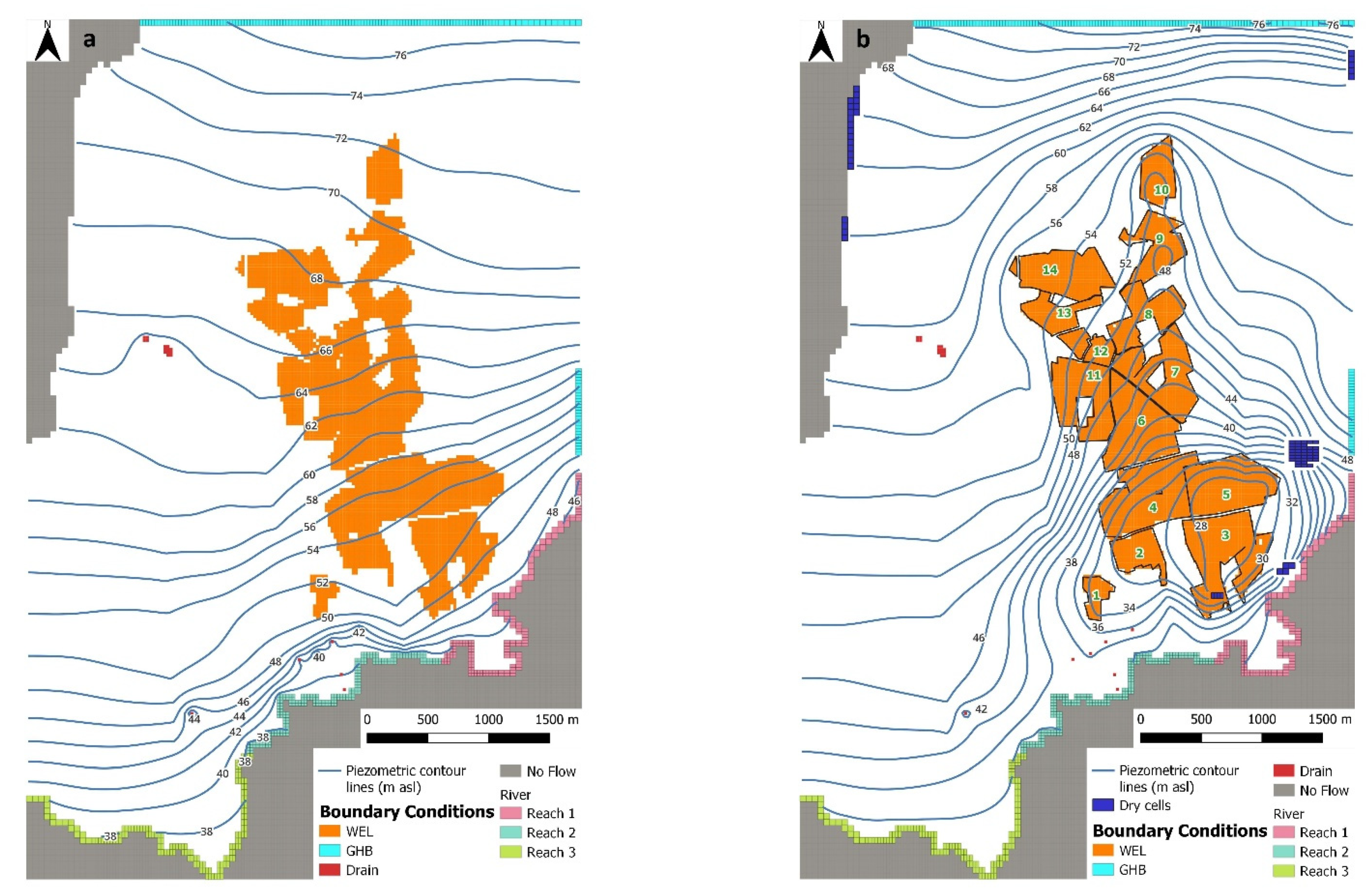
General Head Boundary (GHB): this condition, assigned to the northern limit of the model to Layers 1 and 3 and to a portion of the eastern border, was used to simulate head-dependent inflows into the system. Head values of GHB were derived from the potentiometric surface map available for the area under natural conditions [40], i.e., when withdrawals from the quarry area were limited;

-

No Flow boundary: this condition was assigned to the northwestern limit of the model, where null exchange between the plain and the surrounding reliefs has been recognized [33,34]; the same condition was also assigned to the southern sector of the model beyond the Aniene River, which does not affect the investigated system;

-

DRAIN: this head-dependent flux boundary allows the outflow from the system. This condition was applied to the stress periods SP1, SP2 and SP3 (see below) to the Regina, Colonnelle (Acque Albule springs) and S. Giovanni lakes and to the minor springs located in the southern sector of the study area; the drain condition was also applied to simulate the drainage from the quarries during the calibration process for stress period SP2;

-

RIVER: this condition simulates the water exchanges between river and groundwater. This condition was assigned to the southern boundary of the model where the Aniene River flows, taking into account the elevations of the river and distinguishing three different conductance zones during calibration process (named as Reach 1, Reach 2 and Reach 3).

Simulation time was subdivided into two stress periods: the first stress period (SP1) simulates the undisturbed conditions, not influenced by the massive pumping performed in the quarry area, while the second stress period (SP2) refers to system conditions affected by the dewatering activities in 2008. Given the length of each stress period and the high hydraulic diffusivity of the aquifer, it is assumed that the system reaches a steady-state condition for each stress period. Consequently, the two stress periods were set as steady-state periods in sequence.

Direct meteoric recharge on the modeled area was based on data of the Tivoli meteorological station recorded between 1951 and 2008. Brunetti et al. [34] report an average annual precipitation of 863 mm and an average annual air temperature of 15.7 °C. The same authors assessed a meteoric recharge value equal to 275 mm/year for the plain. The reliability of the adopted data was also validated by values recorded from the same meteorological station after 2008 to date. The starting average annual meteoric recharge value of 275 mm/year was then assigned to the modeled area, multiplied by a factor that considers the rainfall and temperature trends, as described in Mangianti and Leone [41]. Thus, a multiplying factor of 1.1 was applied to the meteoric recharge for SP1 and 0.9 to SP2.

The pre-calibration hydraulic conductivity values for the three layers were assigned on the basis of the available values of the transmissivity [33,34] and thickness of aquifer. In Layer 2, an additional pattern of hydraulic conductivity discretized the main faults and fractures, given their fundamental role in the exchanges between the overlapping aquifers. The initial horizontal hydraulic conductivity values assigned to each layer are listed in

Table 1. Initial values of horizontal hydraulic conductivities (k_h).

Layer	Initial kh Values (m/s)
Layer 1: Travertine aquifer	1 × 10−3
Layer 2: Aquitard	1 × 10−6
Layer 2: Fault zone	1 × 10−2
Layer 3: Carbonate aquifer	1 × 10−3

; the vertical hydraulic conductivity was set equal to 1/10 of the horizontal one.

The calibration process was developed using the PEST_HP code [36,37] associated with the use of pilot points [42,43], varying the hydraulic conductivity, conductance and water level of GHB, conductance of RIVER reaches and conductance of DRAIN. Tikhonov regularization [44] was used to include the conceptual “soft knowledge” model as prior information and to constraint the parameters’ variation along the history-matching process. This mathematical regularization makes the values of the parameters deviate as little as possible from a preferred value, unless they are in contrast with observed data.

History matching and sensitivity analysis were based on the available potentiometric map of the travertine aquifer, representative of the undisturbed conditions [40], and the most complete potentiometric reconstruction recorded in 2008, representative of the stressed aquifer conditions [45]. Specifically, 23 and 70 water level measurements were considered for undisturbed and stressed conditions, respectively. The average pre-development spring flow rates and the single-target flow rate of the Acque Albule springs under the dewatering conditions were included as observations as well. Uncertainty of the data and measurement noise were assessed in order to set an objective function with a lower threshold along the calibration process.

The model with adjusted parameters was then used to qualitatively examine the relationship between the dewatering flow from the quarry area and the discharge response of the Acque Albule springs and the Aniene River. Specifically, a scenario representing the configuration of the quarry area in 2020 was simulated (SP3), corresponding to the maximum extent of the quarry area. In this case, the dewatering activities from quarries were represented by a specified flux boundary condition (WEL), covering an extension arbitrarily set equal to the authorized concession area for travertine extraction (Figure 3). The abstraction from the quarry area was iteratively determined in order to obtain a drawdown of the groundwater level equal to the project excavation depth in the quarries. In this way, the actual maximum pumping scenario was set up.

4. Results

4.1. Variation of the Groundwater Flow and Level in the Plain

The reconstruction of the hydrogeological history of the Acque Albule Basin was first carried out by examining the flow rates of the springs and of dewatering from the quarry area. Figure 4 shows the available flow measurements published in [25,26,32,46,47] and unpublished studies compared with those determined in 2020 for the Acque Albule springs, other minor springs (Barco and Bretella springs) and quarry outflow channels. Although the flow measurements are sporadic and not continuous, the flow decrease of the Acque Albule springs and other minor springs over time is indisputably related to the simultaneous increase in the dewatering from the quarry area. Since 2001, the natural outflow at the surface of the Acque Albule springs has become nearly zero.

As already known in the literature [22,23] and as confirmed by the surveys carried out in 2020, the comparison between the physico-chemical parameters and chemical composition of the drainage water of the quarries and spring water (Acque Albule and minor springs) clearly shows that they are fed by the same groundwater resource (see Figure 1c). As shown in

Table 2. Literature and 2020 Temperature (T) and Electrical Conductivity (EC) values measured within the plain.

Year	Acque Albule Springs		Bretella Spring		Barco Springs		Quarries
	T (°C)	EC (µS/cm)	T (°C)	EC (µS/cm)	T (°C)	EC (µS/cm)	T (°C)	EC (µS/cm)
2005 a	23.7	3610	21.1	2614			19.9–23.5	2640–3360
2008 b	22.2	3460			21.0–22.0	2920–3260	17.6–23.3	1550–3400
2020 c	23.5	3611	20.5	2759	20.9–22.1	3180–3360	19.0–21.4	3140–3230

^a [28], ^b [23] ^c present study.

, comparable temperature (T) and electrical conductivity (EC) values result for the drainage water of the quarries and for the waters emerging from the springs.

The impact of the quarries’ dewatering on the groundwater flow rate of the plain is widely documented in the available published studies [33,34] and technical reports [28,46,47]. The monitoring of water levels carried out from 2005 to 2009 [47] at observation points around the Acque Albule springs, while the flow to the surface from these springs was significantly decreasing, is meaningful in this regard. During the observation period, the water level with a longer time series shows a general decline over time and an immediate response to the pumping from the quarry area. An example of the general trend of groundwater level in two piezometers located, respectively, near Regina Lake (S1 in Figure 2) and about 900 m South of the Acque Albule springs (S2 in Figure 2) is shown in Figure 5, together with the periods of interruption of or reduction in the pumping flow from the quarry area. Although the pumping rate from the quarry area is not known during the monitoring period, the immediate response of the groundwater level to temporary interruption of or reduction in pumping from the quarry area is clear. This evidence, together with the measurements made in 2020, show a decline in water level of about 4 m in the period 2005–2008 and of about 5 m in the period 2003–2020 for Regina Lake; S. Giovanni Lake waters decreased by about 7 m in the period 2003–2020.

The fluctuations in the water level of Regina Lake on a daily scale in the spa season period overlap with the general trend of the water level [47]. These fluctuations are due to the pumping from the lake to supply the thermal plant since 2002, when the Acque Albule springs no longer gave significant flow to the surface. Even in this case, there is an immediate response to the pumping of the water level of the lake, as shown in Figure 6.

If the Cooper and Jacob [48] model is used to interpret the data, the drawdown and recovery of the lake water level versus time can be considered, providing a good adaptation of the measured data during the daily fluctuations to the theoretical model. Considering the flow rate pumped from the lake (from 500 to 700 L/s), an estimate of the transmissivity of 0.1–0.2 m²/s is obtained. These transmissivity values are in agreement with those obtained from pumping tests carried out in the travertine aquifer (0.2 m²/s in [22]), explaining the immediate response of the aquifer to pumping and the significant propagation of the drawdown in the aquifer’s under-development condition.

4.2. Results of Groundwater Modeling

The historical data of the Acque Albule Basin were assimilated by the model to represents two important hydrogeological situations, the pre- and under-development conditions.

The results of the coupled calibration of stress periods SP1 and SP2 are represented by the possible hydraulic conductivity fields of Layers 1 and 2 (for Layer 3, a uniform calibrated value was kept) and by the conductance values of the river, drains and GHB boundary conditions (Figure 7 and

Table 3. Calibrated parameter values.

Parameter	Calibrated Values
Acque Albule springs conductance	2.94 × 10−2 (m2/s)
Minor springs conductance	5.43 × 10−1 (m2/s)
River conductance—Reach 1	5.56 × 10−3 (m2/s)
River conductance—Reach 2	1.05 × 10−1 (m2/s)
River conductance—Reach 3	1.52 × 10−3 (m2/s)
Northern GHB conductance	2.60 × 10−3 (m2/s)
Northern GHB elevation	80.3 (m asl)

). The spatial distribution of the hydraulic conductivity was estimated in 268 pilot points in the first layer, eight discrete faults, plus 117 pilot points, in the second layer and by a uniform value in the third layer. The obtained parameters minimize the error between the simulated and observed values of the hydraulic heads and flow rates, in a way that deviate as little as possible from the provided prior information and that does not reduce the residuals below the measurement noise of the data, which is especially high for the flow measurements.

The comparison between the observed and simulated values of the hydraulic heads related to Layer 1 for undisturbed (SP1) and stressed conditions (SP2) is shown in Figure 8. Considering 93 observation points, a mean error, root-mean-squared error (RMSE) and normalized RMSE of 0.20 m, 2.16 m and 3.8% result, respectively. The comparison of the observed and simulated flow rate values is shown in

Table 4. Comparison of observed and simulated flow rates in m³/s of the calibrated model for SP1 and SP2.

Flow Rates (m3/s)	Observed Value	Simulated Value	Residual
Acque Albule springs SP1	2.50	1.88	0.62
Acque Albule springs SP2	0.01	0.17	−0.16
Minor springs SP1	0.80	0.69	0.11
Minor springs SP2	0.20	0.12	0.08
Drainage from quarries SP2	4.67	6.03	−1.36
Northern GHB SP1	4.00	3.96	0.04

. In this case, there are more significant deviations (mean error of 0.16 m³/s, an RMSE of 0.52 m³/s and a normalized RMSE of 7.6%), which are linked to the sporadic and instantaneous flow measurements, as well as to the necessary simplifications of the model.

The sensitivity analysis was performed at the beginning of the calibration process, using the Jacobian matrix calculated by PEST_HP (also called the sensitivity matrix, calculated as explained in [36]). The conductance of the GHB northern inflow boundary and of the Acque Albule drain presents the highest sensitivities. The other conductance parameters and those of hydraulic conductivity (represented by pilot points) have sensitivities one or two orders of magnitude lower, as shown in

Table 5. Composite sensitivity values for each parameter.

Parameter	Composite Sensitivity
Acque Albule springs conductance	0.30
Minor springs conductance	3.07 × 10−2
River conductance—Reach 1	5.30 × 10−2
River conductance—Reach 2	2.55 × 10−3
River conductance—Reach 3	1.71 × 10−2
Northern GHB conductance	0.75
Northern GHB level	5.18 × 10−2
Average sensitivity of pilot points	2.50 × 10−2

. These facts highlight that the northern boundary of the model is strongly influenced by hydraulic stresses induced by the pumping from the quarries, although it is about 2 km upstream from the quarry area.

The calibrated model was then used to simulate the maximum extension and deepening of the travertine quarries, represented in the stress period SP3. To this end, the quarry concessions active in 2020 were considered; they cover a surface area of about 3 km², with a project excavation depth ranging between 12 and 30 m. The several authorized quarries (about 50) were grouped into 14 groups (Figure 9b), based on the depth of excavation and the proximity of pumping stations. The grouping of quarries made it possible to determine the pumping rate from each quarry group necessary to induce a drawdown reaching the project excavation floor. The resulting total flow of dewatering from the quarry area is in accordance with the flow measured in 2020 in the outflow channels (i.e., approximately 6 m³/s).

The simulation results under maximum dewatering (SP3) were then compared with those of the undisturbed conditions (SP1) in terms of potentiometric surfaces (Figure 9) and water budget (

Table 6. Water budget for the model.

Term	SP1				SP3
	Inflow		Outflow		Inflow		Outflow
	m3/s	%	m3/s	%	m3/s	%	m3/s	%
Meteoric recharge	0.32	7.4			0.24	3.5
GHB North, Layer 1	1.04	24.1			2.01	29.1
GHB North, Layer 3	2.92	67.8			3.99	57.7
GHB Est			0.05	1.1	0.06	0.9
Aniene River	0.03	0.7	1.70	39.4	0.61	8.8	0.50	7.4
Quarry dewatering							5.98	88.3
Acque Albule springs			1.88	43.5			0.18	2.7
Minor springs			0.69	16.0			0.11	1.6
Total	4.31	100	4.32	100	6.91	100	6.77	100

).

As shown in Figure 9, a significant deformation of the groundwater flow pattern of the travertine aquifer is evident for the under-development conditions. The lowering of the piezometric level in the quarry area, up to 26 m, induces an increase in the hydraulic gradient at the northern portion of the plain and a local inversion of flow between the groundwater and surface water of the Aniene River. In the under-development conditions, the inflow from the northern boundary increases 50% and the flow towards the Aniene River decreases about 30% in order to partially compensate for the pumping from the area of the quarries (Table 6). In addition, the exchanges between the deeper carbonate aquifer (Layer 3) and the travertine aquifer (Layer 1) change from SP1 to SP3, increasing from 1.69 m³/s in the undisturbed conditions to 3.78 m³/s in the under-development conditions. The abstraction of groundwater from the quarry area also causes a remarkable reduction in the flow rate from the springs of about 90%, in accordance with the measurements made in 2020 and the last 20 years, also triggering a meaningful inflow from the river towards the aquifer (of about 10% of the total inflow). In addition, a reduction in the storage of the aquifer occurs between the pre- and under-development conditions. A rough estimate can be assessed taking into account the drawdown between the two conditions and the specific yield of the travertine aquifer. Assuming a specific yield value of 0.05, based on the few available pumping tests [22] and the effective porosity values of the travertines and fractured limestones reported in the literature [49,50,51], there is a storage decrease of approximately 13 × 10⁶ m³ over 40 years. This value corresponds to 24% of the total storage of the travertine aquifer, estimated considering the same specific yield value and the saturated volume of the aquifer under natural conditions (represented by the SP1).

The results of the stress period SP1, representative of the pre-development conditions, and of the stress period SP3, representative of the maximum planned withdrawals from the quarry area, were subsequently used to analyze the response of the aquifer to the dewatering from the quarry area.

Different dewatering scenarios were simulated (

Table 7. Simulated scenarios by varying the total pumping flow rate from quarries (Q_tq).

Scenarios	Qtq (m3/s)	% SP3
SP1	0	0
SP3-30	1.80	30
SP3-50	2.99	50
SP3-70	4.18	70
SP3-80	4.78	80
SP3	5.97	100

), gradually and homogeneously reducing the pumping from the different groups of quarries and verifying the variation in the flow rate of the Acque Albule springs, of the minor springs, flow towards the river and inflow from the northern boundary GHB. By varying the total flow rate from the quarry area (Q_tq) between 0 and about 6 m³/s, the results represented in Figure 10 were obtained. Regardless of the specific flow values shown in the diagram, the results highlight linear relationships between the total pumping flow from the quarry area and springs and river discharge with negative slope coefficients, and inflow from the northern boundary with positive slope coefficients. The graph also shows that there is a threshold of the pumping rate from the quarry area for which the reversal of the flow between the aquifer and river occurs (river with negative discharges in Figure 10).

The variation of the total dewatering flow implies a different variation of the drawdown in the different groups of quarries. As shown in Figure 11, a quadratic regression results between the two variables:

Δh_i = a + b (∑Q_i) + c (∑Q_i)²

where:

-

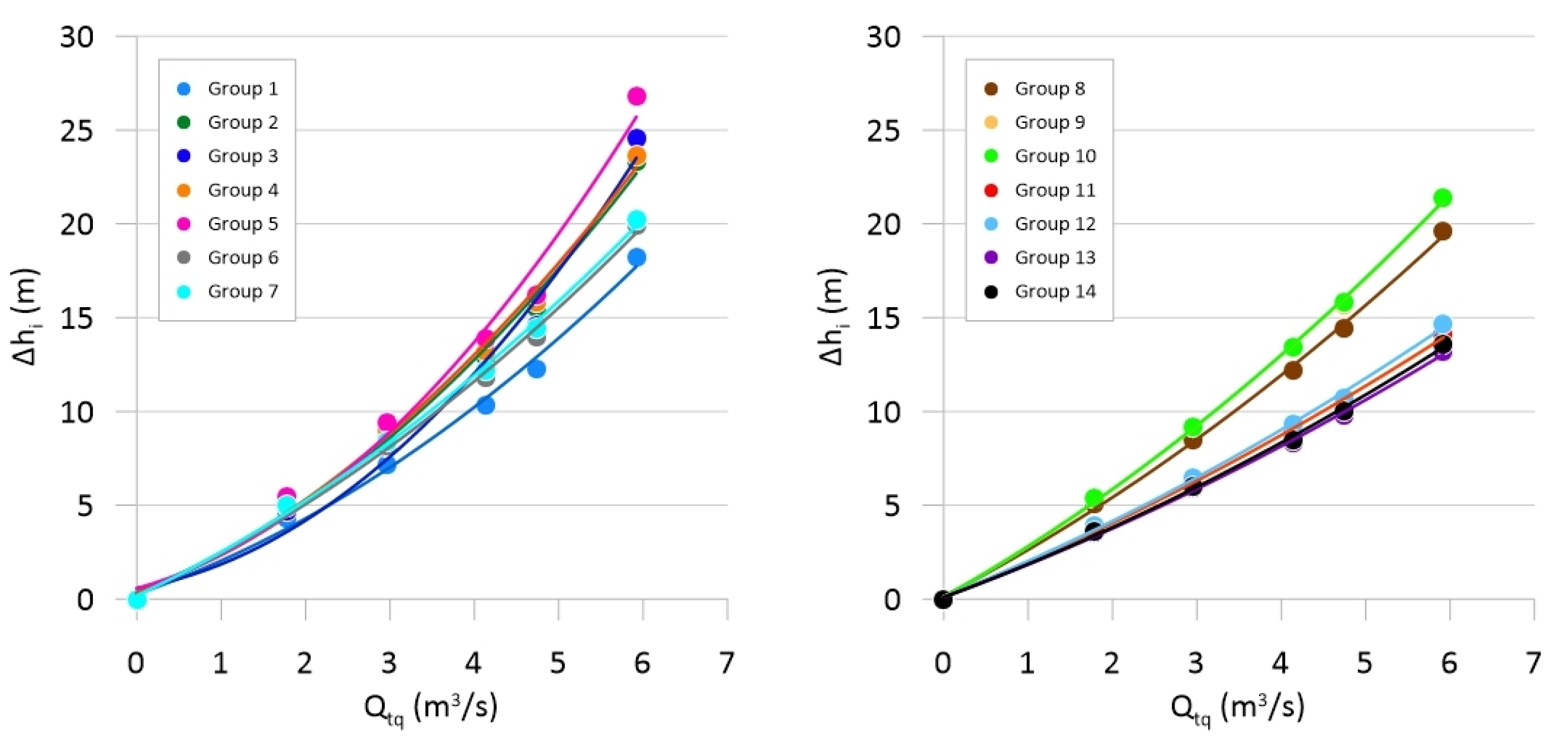
Δh_i is the drawdown in the i-th group of quarries,

-

Q_i is the dewatering discharge from the i-th group of quarries,

-

a, b and c are coefficients depending on the location of the group in the groundwater flow pattern, the pumping rate from each group and the interference of pumping from the adjacent groups.

In order to examine the influence of the single group of quarries on the plain’s main discharge areas of groundwater, represented by the Acque Albule springs and the river, additional scenarios were outlined (14 simulations for four pumping rate variations from each group). These included the progressive reduction in the flow from the i-th group of quarries from the maximum flow down to zero, keeping the other groups active at the maximum pumping rate. Two indices were considered to verify the influence of the single group on the flow of the springs and river:

$$I{Q}_s=1-\frac{Q_{s SP1}-Q_i}{Q_{s SP1}-Q_{s SP3}}$$

where:

-

IQ_s is the increase in flow of the Acque Albule spring in response to the variation of pumping rate from the i-th group of quarries,

-

Q_sSP1 is the flow discharge of the Acque Albule springs under natural conditions,

-

Q_sSP3 is the flow discharge of the Acque Albule springs with maximum pumping from all groups of quarries,

-

Q_i is the pumping flow from the i-th quarry

and:

$$I{Q}_r=1-\frac{Q_{r SP1}-Q_i}{Q_{r SP1}-Q_{r SP3}}$$

-

IQ_r is the increase in flow of the Aniene River in response to the variation of the pumping rate from the i-th group of quarries,

-

Q_rSP1 is the flow discharge towards the Aniene River under natural conditions,

-

Q_rSP3 is flow discharge toward the Aniene River with maximum pumping from all groups of quarries.

The results of the simulations are shown in Figure 12: linear relations between IQ_s and Q_i and between IQ_r and Q_i for the different groups were observed. The flow of the Acque Albule springs is mainly affected by the groups of quarries characterized by a higher flow rate located in the central and southern sectors of the travertine extraction zone (groups 2, 3, 5, 9 and 10 in Figure 9b). The flow towards the river is mainly affected by the distance of the pumping center from the stream, as well as the amount of pumping from different groups (groups 2, 3 and 5 in Figure 9b).

5. Discussion

In the Tivoli plain, the quarries drain the same waters that feed (or fed, in the past) the springs, as highlighted from their physico-chemical parameters and chemical composition (Figure 1c and Table 2). Therefore, the extraction of groundwater from the quarries impacts the same resource that supplies the spa industry.

The results obtained from the analysis of the hydrogeological history and of the groundwater modeling of the system allow us to infer significant elements regarding the sustainability of the abstractions from the quarry area, on the basis of the current local use of groundwater resources. Although there is a lack of continuous and effective monitoring of the outflow from the system and the groundwater modeling results suffer from uncertainty, the main factors affecting sustainable yield can be determined. These factors can be identified by comparing the different conditions of the system, i.e., the pre- and under-development conditions.

On the scale of a generalized hydrogeological system, under pre-development conditions, a steady-state equilibrium prevails where the natural recharge (R₀) equals the natural discharge (D₀) on an annual average balance (Figure 13):

R₀ = D₀

(1)

For the studied system, according to the estimate of the water budget of the travertine aquifer under natural conditions, the term R₀ is approximately 4.3 m³/s. The term R₀ is given by:

R₀ = R_l + R_d

where R_l is the recharge of the travertine aquifer both laterally from the reliefs surrounding the plain and from the bottom by the buried carbonate aquifer, and R_d is the direct meteoric recharge on the plain. In Equation (1), the term D₀ is given by:

D₀ = D_s + D_f

where D_s is the flow rate of the springs in the plain and D_f is the groundwater flow discharging in the Aniene River. R_l provides the main contribution to R₀, approximately 92%, when compared to the term R_d, approximately 7%. R₀ is equivalent to the term D₀, to which D_s provides the main contribution, approximately 60%, if compared to the term D_f, approximately 39% (Table 6).

When a general system is subjected to a groundwater withdrawal P (Figure 13):

(R₀ + ΔR₀) − (D₀ − ΔD₀) − P = ΔV/Δt

(2)

where ΔR₀ represents an increase in natural recharge, ΔD₀ a decrease in natural discharge, P the withdrawal and ΔV/Δt a change of aquifer storage over time [52]. Equation (2) may also be written as:

ΔR₀ + ΔD₀ − P = ΔV/Δt

(3)

When the variation in storage approaches zero, a new equilibrium is reached in the system after the application of pumping, P, depending on the so-called “capture” [11,53]:

P = ΔR₀ + ΔD₀

(4)

that is, P depends on the sum of the increase in natural recharge and the decrease in natural discharge. After pumping activation, at equilibrium, the groundwater discharge from the system is reduced; therefore, the residual discharge D_r is obtained:

D_r = D₀ − ΔD₀

(5)

or:

ΔD₀ = D₀ − D_r

(6)

and by replacing D₀ with R₀ in Equation (6), Equation (4) can be rewritten as follows:

P = R₀ + ΔR₀ − D_r

(7)

According to Zhou [14], when the system reaches the new steady-state conditions, that is ΔV/Δt = 0, the withdrawals depend on the natural recharge and its increase, and the discharge are decreased (Figure 13).

For the studied system, in the under-development conditions, a significant decrease in the springs’ flow rate and in the groundwater level of the travertine aquifer result from experimental evidence. The latter phenomenon corresponds to the variation in the storage of the travertine aquifer, estimated to be about 24% of the aquifer storage, under natural conditions over 40 years. However, the studied aquifer quickly reaches a new equilibrium condition after the activation of the withdrawals, depending on the hydraulic diffusivity of the aquifer and on the square of the distance of the limits to be captured [52]. Considering the distance of these limits, represented both by the river and the GHB of the northern sector, and the high hydraulic diffusivity of the aquifer (that is of the order of magnitude of 2 m²/s), the aquifer, as a matter of fact, in a few days, reaches a new steady-state condition under every new pumping stress.

The terms of Equation (7) can be specified for the case study (Figure 13) on the basis of measurements and numerical simulations. Specifically, the term P, mainly attributable to the dewatering from the quarry area, is equal to about 6.0 m³/s, namely about 88% of the total outflow from the system in under-development conditions (Table 6). The increase in recharge (ΔR₀) is approximately 2.5 m³/s and is mainly due to inflow from the northern GHB boundary (nearly the 88% of the total inflow). The residual discharge from the system (D_r) is around 0.8 m³/s, representing about 12% of the total outflow from the system, a significant reduction in the natural outflow in under-development conditions if compared to pre-development conditions (ΔD₀ is approximately of 3.5 m³/s).

Theoretically, the “maximum sustainable yield” of a system corresponds with D_r = 0; any withdrawal above the maximum sustainable yield implies a progressive depletion of groundwater storage [12]. Although at the system scale the residual outflow is greater than 0 for the maximum groundwater withdrawal simulated by SP3, if the natural discharge areas of the system are specifically considered, the maximum withdrawal appears unsustainable. In fact, the natural outflow from the Acque Albule springs has been practically close to zero since the 2000s, and the total outflow towards the Aniene River is decreased by 70% compared to natural conditions, according to the simulations, particularly in the easternmost stretch of the river, where flows to the aquifer are triggered by dewatering (for approximately 9% of the total recharge of the system in under-development conditions). The first condition, i.e., the absence of significant natural flow from the Acque Albule springs, represents a hydrogeologically and environmentally unsustainable situation that also has economic and administrative consequences. In fact, currently, the thermal plant is forced to pump water from the karst lake to meet the needs of the spa, increasing costs during the period of activity. In addition, the concession of thermal waters issued by the local authority states the exclusive use of the thermal waters of the basin. The second condition, namely the reversal of flow from the river to the aquifer in the stretch of river close to the quarry area, could lead to a qualitative decline in the hydrothermal resource, declassifying the thermal waters used for therapeutic purposes in the spa.

It follows that the most stringent constraints to ensure the sustainable yield of the system must be identified in the residual outflow to the Acque Albule springs and river, specifically: (i) the residual outflow to the Acque Albule springs should be greater than or equal to 0.7 m³/s, in order to ensure the necessary resources for the thermal plant activities without additional costs for pumping and to restore the dependent groundwater ecosystem of the springs; (ii) no inflow from the river to the aquifer should take place so as to maintain the quality of the thermal waters.

Compliance with these constraints necessarily implies a significant limitation of the withdrawal from the quarry area, which results in a reduction in the depth of excavation for the extraction of travertine. This becomes a problem for the local economic activity due to the reduction in the volume of travertine to be extracted. In the absence of a continuous and effective monitoring of groundwater levels and flows of the plain and of specific on-site tests, it is not possible to define in detail the amount of sustainable yield from the quarry area. However, it is clear from the study that a new location of the extraction area can help to contain the economic loss linked to the reduction in the excavation depth. On the basis of the scenarios outlined to verify the effect of pumping rate variations of the single group of quarries on the flow of the springs and the river (Figure 12), the quarry groups of the central and southern are, in fact, the most impacting ones. In other words, extending the quarry area to the northeast, the northern GHB limit would preferentially be captured, and limiting the extent of the quarry zone in the southern sector close to the river can allow us to reach a point of equilibrium between the constraints of sustainability and the economic interests of the quarrying activity, given the current use of the groundwater resource.

6. Conclusions

The case study seems to be significant since it analyzes the applicability of the concept of sustainable yield in a complex hydrogeological system. In the Acque Albule Basin, the coexistence of a massive dewatering for the extraction of travertine, coupled with an important thermal spring supplying a famous and popular spa, puts the two profitable economic activities resting on the same groundwater resource into conflict. The withdrawal of groundwater from the quarry area has had a significant impact on the water balance of the hydrogeological system. An increase in inflow from surrounding carbonate aquifers and a decrease in storage and in natural discharge of the travertine aquifer result in under-development conditions.

The study highlights the system’s fast response to the stress of pumping due to the high hydraulic diffusivity of the aquifer. Therefore, the aquifer quickly reaches new equilibria after the activation of the massive withdrawal. For these hydrogeological conditions, the residual discharge towards the main discharge areas of the system (the springs and river) is very sensitive to the pumping flow rate, according to an inverse linear relationship, and represents an efficient indicator for sustainability when assessing groundwater withdrawals. To maintain a sufficient residual discharge to the natural outflow areas of the system, to preserve the ground–surface water relationship and thus to contain the qualitative decay of groundwater, in addition to withdrawal amount, the position of the pumping center in the groundwater flow net and its distance from boundaries to be captured becomes crucial. These findings lay the essential foundations for developing sustainable management models of groundwater resources. A sustainable management plan of the different uses of this resource of the plain (thermal waters, surface water, travertine, site of nature conservation, etc.) clearly requires a more extensive analysis, including economic, environmental and social assessments. However, to reduce the current impact on groundwater resources, the depth of extraction and position of quarries within the groundwater flow pattern seem to be the key factors to be considered.

In more general terms, the results show that the definition of sustainable yield depends on the specificity of the dynamics of the groundwater flow and on the speed at which the system reacts to the application of groundwater withdrawals. When the system is characterized by a high hydraulic diffusivity, an immediate reaction to pumping is prompted. Thus, monitoring the residual outflows from the system becomes an efficient tool, both to verify the measures adopted for sustainable groundwater management and to update and validate the conceptual and numerical models. This approach seems to be more effective than those based on the comparison between recharge and pumping or on the effects of the capture caused by pumping, since it tries to reduce the prediction-specific uncertainties, whose correct perception is an imperative when whatever decision and/or action must be taken in a complex and conflictual hydrogeological contest.

References

1. Alley, M.; Lake, S.A. The journey from safe yield to sustainability. Ground Water 2004, 42, 12–16. [Google Scholar] [CrossRef] [PubMed]
2. Pierce, S.A.; Sharp, J.M.; Guillaume, J.H.A., Jr.; Mace, R.E.; Eaton, D.J. Aquifer-yield continuum as a guide and typology for science-based groundwater management. Hydrogeol. J. 2013, 21, 331–340. [Google Scholar] [CrossRef]
3. Gleeson, T.; Cuthbert, M.; Ferguson, G.; Perrone, D. Global groundwater sustainability, resources, and systems in the Anthropocene. Annu. Rev. Earth Planet. Sci. 2020, 48, 431–463. [Google Scholar] [CrossRef] [Green Version]
4. Elshall, A.S.; Arik, A.D.; El-Kadi, A.I.; Pierce, S.; Ye, M.; Burnett, K.M.; Wada, C.A.; Bremer, L.L.; Chun, G. Groundwater sustainability: A review of the interactions between science and policy. Environ. Res. Lett. 2020, 15, 093004. [Google Scholar] [CrossRef]
5. Alley, W.M.; Reilly, T.E.; Franke, O.L. Sustainability of ground-water resources. US Geol. Surv. Circ. 1999, 1186, 1–79. [Google Scholar]
6. Lee, C.H. The determination of safe yield of underground reservoirs of the closed basin type. Trans. Am. Soc. Civ. Eng. 1915, 78, 148–151. [Google Scholar] [CrossRef]
7. Conkling, H. Utilization of groundwater storage in stream system development. Proc. Am. Soc. Civ. Eng. 1945, 111, 33–62. [Google Scholar]
8. Thomas, H.E. The Conservation of Groundwater; McGraw-Hill Book Company: New York, NY, USA, 1951; p. 327. [Google Scholar]
9. Domenico, P.A. Concepts and Models in Groundwater Hydrology; McGraw-Hill: New York, NY, USA, 1972. [Google Scholar]
10. Sophocleous, M. From safe yield to sustainable development of water resources: The Kansas experience. J. Hydrol. 2000, 235, 27–43. [Google Scholar] [CrossRef]
11. Bredehoeft, J.D. The water budget myth revisited: Why hydrogeologists model. Groundwater 2002, 40, 340–345. [Google Scholar] [CrossRef]
12. Kalf, F.R.; Wooley, D.R. Applicability and methodology of determining sustainable yield in groundwater systems. Hydrogeol. J. 2005, 13, 295–312. [Google Scholar] [CrossRef]
13. Devlin, J.; Sophocleous, M. The persistence of the water budget myth and its relationship to sustainability. Hydrogeol. J. 2005, 13, 549–554. [Google Scholar] [CrossRef]
14. Zhou, Y. A critical review of groundwater budget myth, safe yield and sustainability. J. Hydrol. 2009, 370, 207–213. [Google Scholar] [CrossRef]
15. Konikow, L.F.; Leake, S.A. Depletion and capture: Revisiting “the source of water derived from wells”. Groundwater 2014, 52, 100–111. [Google Scholar] [CrossRef]
16. Faccenna, C. Structural and hydrogeological features of Pleistocene shear zones in the area of Rome (central Italy). Ann. Geofis. 1994, 37, 121–133. [Google Scholar] [CrossRef]
17. Faccenna, C.; Soligo, M.; Billi, A.; De Filippis, L.; Funiciello, R.; Rossetti, C.; Tuccimei, P. Late Pleistocene depositional cycles of the Lapis Tiburtinus travertine (Tivoli, central Italy): Possible influence of climate and fault activity. Glob. Planet. Chang. 2008, 63, 299–308. [Google Scholar] [CrossRef]
18. Pentecost, A.; Tortora, P. Bagni di Tivoli, Lazio: A modern travertine depositing site and its associated microorganism. Boll. Soc. Geol. It. 1989, 108, 315–324. [Google Scholar]
19. Minissale, A.; Kerrick, D.M.; Magro, G.; Murrell, M.T.; Paladini, M.; Rihs, S.; Sturchio, N.C.; Tassi, F.; Vaselli, O. Geochemistry of Quaternary travertines in the region north of Rome (Italy): Structural, hydrological and paleoclimatic implications. Earth Planet. Sci. Lett. 2002, 203, 709–728. [Google Scholar] [CrossRef]
20. Billi, A.; Valle, A.; Brilli, M.; Faccenna, C.; Funiciello, R. Fracture-controlled fluid circulation and dissolutional weathering in sinkhole-prone carbonate rocks from central Italy. J. Struct. Geol. 2006, 29, 385–395. [Google Scholar] [CrossRef]
21. La Vigna, F.; Mazza, R.; Capelli, G. Detecting the flow relationships between deep and shallow aquifers in an exploited groundwater system, using long-term monitoring data and quantitative hydrogeology: The Acque Albule basin case (Rome, Italy). Hydrol. Process. 2013, 27, 3159–3173. [Google Scholar] [CrossRef]
22. Petitta, M.; Primavera, P.; Tuccimei, P.; Aravena, R. Interaction between deep and shallow groundwater systems in areas affected by Quaternary tectonics (Central Italy): A geochemical and isotope approach. Environ. Earth Sci. 2010, 63, 11–30. [Google Scholar] [CrossRef]
23. Carucci, V.; Petitta, M.; Aravena, R. Interaction between shallow and deep aquifers in the Tivoli Plain (central Italy) enhanced by groundwater extraction: A multi-isotope approach and geochemical modeling. Appl. Geochem. 2012, 27, 266–280. [Google Scholar] [CrossRef]
24. Boni, C.; Bono, P.; Capelli, G. Schema idrogeologico dell’Italia Centrale. Mem. Soc. Geol. It. 1986, 35, 991–1012. [Google Scholar]
25. Capelli, G.; Cosentino, D.; Messina, P.; Raffi, R.; Ventura, G. Modalità di ricarica e assetto strutturale dell’acquifero delle sorgenti Capore—S. Angelo (Monti Lucretili—Sabina Meridionale). Geol. Romana 1987, 26, 419–447. [Google Scholar]
26. Capelli, G.; Mazza, R.; Taviani, S. Studi idrogeologici per la definizione degli strumenti operativi del piano stralcio per l’uso compatibile delle risorse idriche sotterranee nell’ambito dei sistemi acquiferi prospicienti i territori vulcanici laziali; Università degli Studi di Roma Tre: Roma, Italy, 2005; Unpublished work. [Google Scholar]
27. Cosentino, D.; Pasquali, V. Carta Geologica Informatizzata della Regione Lazio; Università degli Studi Roma Tre—Dipartimento di Scienze Geologiche, Regione Lazio—Agenzia Regionale Parchi—Area Difesa del Suolo: Roma, Italy, 2012. [Google Scholar]
28. Acque Albule S.p.A. Indagini Idrogeologiche per Determinare Le Cause dei Dissesti Agli Edifici di via Cesare Augusto e Aree Limitrofe, in Località Bagni di Tivoli; Bono, P., Ed.; Technical Report; Università degli Studi di Roma La Sapienza: Roma, Italy, 2005. [Google Scholar]
29. Della Porta, G.; Croci, A.; Marini, M.; Kele, S. Depositional architecture, facies character and geochemical signature of the Tivoli travertines (Pleistocene, Acque Albule Basin, Central Italy). Res. Paleontol. Stratigr. 2017, 123, 487–540. [Google Scholar] [CrossRef]
30. Maxia, C. Il Bacino delle Acque Albule (Lazio). Contr. Sc. Geol. Suppl. Ric. Sc. 1950, 20, 3–20. [Google Scholar]
31. Del Bon, A.; Sbarbati, C.; Brunetti, E.; Carucci, V.; Lacchini, A.; Marinelli, V.; Petitta, M. Groundwater flow and geochemical modeling of the Acque Albule thermal basin (Central Italy): A conceptual model for evaluating influences of human exploitation on flowpath and thermal resource availability. Cent. Eur. Geol. 2015, 58, 152–170. [Google Scholar] [CrossRef]
32. Lombardi, L. Studio idrogeologico del Bacino delle Acque Albule. Roma, Italy, 2005; Unpublished work. [Google Scholar]
33. La Vigna, F.; Hill, M.C.; Rossetto, R.; Mazza, R. Parameterization, sensitivity analysis, and inversion: An investigation using groundwater modeling of the surface-mined Tivoli-Guidonia basin (Metropolitan City of Rome, Italy). Hydrogeol. J. 2016, 24, 1423–1441. [Google Scholar] [CrossRef]
34. Brunetti, E.; Jones, J.P.; Petitta, M.; Rudolph, D.L. Assessing the impact of large-scale dewatering on fault-controlled aquifer systems: A case study in the Acque Albule basin (Tivoli, central Italy). Hydrogeol. J. 2013, 21, 401–423. [Google Scholar] [CrossRef]
35. Harbaugh, A.W. MODFLOW-2005, the U.S. Geological Survey Modular Ground-Water Model—The Ground-Water Flow Process: U.S.; Geological Survey: Reston, VA, USA, 2005; p. 6-A16. [Google Scholar]
36. Doherty, J. Calibration and Uncertainty Analysis for Complex Environmental Models; Watermark Numerical Computing: Brisbane, Australia, 2015. [Google Scholar]
37. Doherty, J. PEST_HP, PEST for Highly Parallelized Computing Environments; Watermark Numerical Computing: Brisbane, Australia, 2021; pp. 1–94. [Google Scholar]
38. Rumbaugh, J.O.; Rumbaugh, D.B. Guide to Using: Groundwater Vistas—Version 8; Environmental Simulation Inc.: Leesport, PA, USA, 2020; pp. 1–515. [Google Scholar]
39. Ciotoli, G.; Meloni, E.; Nisio, S. Studio di sintesi e analisi geospaziale applicata alla valutazione della suscettibilità da sinkholes naturali nella Piana delle Acque Albule (Tivoli, Roma). Mem. Descr. Carta Geol. It. 2015, 99, 203–220. [Google Scholar]
40. Camponeschi, B.; Nolasco, F. Le Risorse Naturali della Regione Lazio; Istituto di Geologia Applicata: Roma, Italy, 1980; pp. 1–423. [Google Scholar]
41. Mangianti, F.; Leone, F. Analisi climatica delle temperature e delle precipitazioni a Roma. In La Geologia di Roma dal centro storico alla periferia. Memorie Descrittive della Carta geologica d’Italia 2008, 80, 169–186. [Google Scholar]
42. Certes, C.; de Marsily, G. Application of the pilot-points method to the identification of aquifer transmissivities. Adv. Water Resour. 1991, 14, 284–300. [Google Scholar] [CrossRef]
43. Doherty, J.; Fienen, M.N.; Hunt, R.J. Approaches to Highly Parameterized Inversion: Pilot-Point Theory, Guidelines, and Research Directions; SIR 2010-5168; US Geological Survey Scientific Investigations Report: Middleton, WI, USA, 2011.
44. Tikhonov, A.N.; Arsenin, V.Y. Solutions of Ill-Posed Problems; Halsted Press: New York, NY, USA, 1977; p. 258. [Google Scholar]
45. La Vigna, F. Modello Numerico del Flusso Dell’unità Idrogeologica Termominerale Delle Acque Albule (Roma). Ph.D. Thesis, Università degli Studi Roma Tre, Roma, Italy, 2009. [Google Scholar]
46. Acque Albule S.p.A. Idrometria del Sistema Acquifero dei Travertini Della Piana di Guidonia-Tivoli: Aggiornamento Dati, Interpretazione Preliminare e Commenti; Bono, P., Ed.; Technical Report; Università degli Studi di Roma La Sapienza: Roma, Italy, 2006. [Google Scholar]
47. Acque Albule S.p.A. Breve Resoconto Sul Monitoraggio Della Falda Ipotermale di Bagni di Tivoli; Bono, P., Ed.; Technical Report; Università degli Studi di Roma La Sapienza: Roma, Italy, 2010. [Google Scholar]
48. Cooper, H.H.; Jacob, C.E. A generalized graphical method for evaluating formation constants and summarizing well field history. Am. Geophys. Union Trans. 1946, 27, 526–534. [Google Scholar] [CrossRef]
49. Custodio, E.; Llamas, M.R. Hidrologìa Subterrànea; Ediciones Omega: Barcelona, Spain, 1983. [Google Scholar]
50. Civita, M. Idrogeologia Applicata e Ambientale; Casa Editrice Ambrosiana: Torino, Italy, 2005. [Google Scholar]
51. Mancini, A.; Frondini, F.; Capezzuoili, E.; Galvez Mejia, E.; Lezzi, G.; Matarazzi, D.; Brogi, A.; Swennen, R. Porosity, bulk density and CaCO3 content of travertines. A new dataset from Rapolano, Canino and Tivoli travertines (Italy). Data Brief 2019, 25, 104158. [Google Scholar] [CrossRef]
52. Theis, C.V. The source of water derived from wells. Civ. Eng. 1940, 10, 277–280. [Google Scholar]
53. Bredehoeft, J.D. Safe yield and the water budget myth. Groundwater 1997, 35, 929. [Google Scholar] [CrossRef]
Figure 1. Setting of the study area. (a) Simplified geological and hydrogeological scheme of the Tivoli plain (mod. from [27,28]); (b) Hydrogeological cross section (A–B) of Tivoli plain (mod. from [21,23,29]): 1—Alluvial deposits, 2—Travertine deposits, 3—Debris deposits, 4—Alluvial, lacustrine and volcanic deposits, 5—Claystone, 6—Carbonate deposits, 7—Groundwater flow direction, 8—Uprising fluids, 9—Springs, 10—Water table level, 11—Faults; (c) Schoeller-Berkaloff diagram of spring, quarry and well waters (mod. from [23]).
Sustainability 14 15248 g001
Figure 2. Thermal water and quarry concession areas, extension of numerical model domain, with locations of the springs, lakes, selected piezometers and drainage canals.
Sustainability 14 15248 g002
Figure 3. Model grid and assigned boundary conditions.
Sustainability 14 15248 g003
Figure 4. Variation over time of the groundwater flows in the Tivoli Plain based on instantaneous, sporadic and non-continuous measurements. Since 2001, the Acque Albule springs reduced their natural outflow at the surface to zero. 2020 measurements were carried out in the present study.
Sustainability 14 15248 g004
Figure 5. Drawdown fluctuations in two piezometers (Δh) during the period April 2005–September 2007, showing the groundwater level response to temporary interruption (red lines) of or reduction (green lines) in pumping from the quarry area (from [47]).
Sustainability 14 15248 g005
Figure 6. Example of daily drawdown–time curve of Regina Lake level (Δh) during the spa season.
Sustainability 14 15248 g006
Figure 7. Distribution of hydraulic conductivity in m/s: (a) horizontal hydraulic conductivity of Layer 1; (b) vertical hydraulic conductivity of Layer 2 (red and green crosses indicate the position of the pilot points).
Sustainability 14 15248 g007
Figure 8. Comparison of observed and simulated hydraulic head values of the calibrated model.
Sustainability 14 15248 g008
Figure 9. Simulated potentiometric surface of the travertine aquifer: (a) for SP1 (pre−development conditions, WEL off); (b) for SP3 (under−development conditions, WEL on; polygons with green numbers indicate quarry groups).
Sustainability 14 15248 g009
Figure 10. Comparison between total pumping flow rate from quarries (Qtq) in different scenarios and Acque Albule (QAB), minor springs (QM_S), river (QRiver) and from northern GHB (QGHB) flow rate variations.
Sustainability 14 15248 g010
Figure 11. Comparison between total pumping flow rate from quarries (Qtq) in different scenarios and drawdown values (Δhi) in each quarry group.
Sustainability 14 15248 g011
Figure 12. Comparison between pumping rate in each quarry group (Qi) and the increase in flow rate of Acque Albule spring (IQs) and Aniene River (IQr).
Sustainability 14 15248 g012
Figure 13. Simplified hydrogeological scheme for pre-development conditions (upper scheme) and under-development conditions (lower scheme). R0: natural recharge; D0: natural discharge; V: volume of aquifer storage; ΔR0: variation in natural recharge; ΔV: change in volume of aquifer storage; Dr: residual discharge; ΔD0: variation in natural discharge.
Sustainability 14 15248 g013