How Big Is the Real Road-Effect Zone? The Impact of the Highway on the Landscape Structure—A Case Study

Abstract

Roads, due to their large spatial scale, significantly affect the landscape, causing numerous and usually irreversible changes. Due to a lack of consensus among various specialists and varying evidence on the extent of the influence of roads, the present study focused on the clarification of the real range of the effect of roads on the environment, especially the landscape structure. The aim of the study was to assess road-effect zones for different types of land use. The existing sections of the European route E30 in the Wielkopolska region (Poland) were selected for the research. Based on buffer analysis, landscape metrics and statistical analysis, such as cluster analysis and changes in mean and variance, the spatial diversity of the landscape and road-effect zone was characterized. The results indicate the spatial diversity of the landscape structure and the range of impact, which depended on the type of land cover. Therefore, to analyze the road-effect zone, it is necessary to take into consideration not only the variable range of impact due to the type of road or the time of exploitation, but also the different types of land use of areas surrounding the road.

1. Introduction

Roads are a large-scale investment causing changes in the environment. The most important impacts of road investment include transforming the structure and functioning of the landscape, excluding part of the land from use, air pollution, noise, soil and crop contamination, surface and underground water pollution, the impact on fauna and flora, as well as human mobility, health and safety [1,2,3,4]. The sustainable development of road infrastructure has to take into account ecological, economic and social issues, as well as spatial management. While from an ecological perspective the effects of roads are mostly negative, the socio-economic effects are mostly positive. Such infrastructure development has been found to improve mobility by increasing access to jobs, facilities and social services, as well as to improve the living conditions of people living near new roads [5,6].

Many of the impacts of roads on the environment are well known, but the problem is to determine the range of these impacts. The range is varied and definitely larger than the road surface or roadside. However, it is not the same for all roads, as it is dependent on the road size and classification, as well as local conditions, the locations and type/purpose of the analysis [7]. According to Komornicki et al. [8], the range of the impact is also determined by the time of road exploitation and the type of surrounding landscape, determined as the slope and land use. Most often, it is asymmetrical [2], and the range of road influence can also be intensified by the increased density of the road network [9].

The area affected by the road—the road-effect zone—has been one of the commonly used approaches to assessing the range of the impact of roads on the environment [10,11]. One of the investigated issues has been the appropriate width of road-effect zones. Despite many studies, there is still no standard procedure to determine the optimal size of road-effect zones [1,12,13]. According to Forman and Deblinger [2], typical road-effect zones have a 100–1000 m range. However, in the existing research, different widths have been used for different purposes. In research related to the impact of roads on animals, the range of road-effect zones depended on the species: 40–2800 m for Dutch birds [14], 1–100 m for salamander [15], 250–1000 m for anuran populations [16], 0–2000 m for steppe birds [17], 1500 and 5000 m for giant panda [18], 50–1000 m for bats [19] and 1–1600 m for the desert tortoise [20]. Some studies also indicated the occurrence of road-effect zones for surface and underground waters and soils [2,21]. In the case of analyses of the landscape structure along roads, the analyzed buffer can have a range of 25–2000 m, depending on the road class [11,13,22], and even 5000 m when assessing changes in the pattern of land use near a highway interchange [23]. For commonly used highways, the range in landscape analyses is 1000 m [12,24]. In all of these studies, the range was the same for both sides of the road, and the areas along the road were treated as homogeneous, ignoring the different types of land use [25].

While many studies in the world have focused on the concept and framework of the impact of roads, only a few case studies have been carried out in Poland. However, the topic of roads seems to be an important issue in Polish strategic documents, where the need to continue road investments has been emphasized. On the other hand, the landscape context was, and still is, an aspect relatively little considered during environmental impact assessments in Poland [26,27,28]. The most comprehensive analysis of the relationship between the road and the landscape was undertaken by Forczek-Brataniec [29,30,31]. Research on this subject has also been carried out by Janeczko [32], Winiarski and Janeczko [33], Nita and Myga-Piątek [26,34], Pukowiec and Pytel [35], Łowicki [36,37], Trzaskowska [38], Janeczko et al. [39] and Lisiak et al. [40], who primarily focused on the assessment of the visual attractiveness of the landscape using GIS tools.

Due to the many previous doubts of various specialists and diverse evidence about the range of road influence, the present work focused on the clarification of the real range of the effect of a road on the environment, especially the landscape structure. Moreover, there is little evidence about the effect of roads on the landscape in terms of the range effect. Hence, our research allows this gap to be filled. The aim of the present study was to assess road-effect zones for different types of land use in a lowland landscape and determine the range of road-effect zones. The article begins with a description of the study area. This section presents information about the Polish section of the European route E30 (the A2 highway). This is followed by a description of materials and methods, where the source of the cartographic data, the applied landscape metrics and the statistical analysis are indicated. The results of the land use classification and buffer analysis, together with the trend analysis for landscape metrics, are described in Section 4. In addition, the change point in the landscape structure based on the statistical analysis is presented. Then, the results are discussed in relation to previous research. Some limitations of the research are also mentioned. Finally, conclusions and recommendations for future work are presented.

2. Study Area

European route E30 from the Republic of Ireland (Cork) to the Russian Federation (Omsk) is an A-Class West–East European route. The Polish section of European route E30 is the A2 highway, well known as the Freedom Highway. It is considered to be one of the most important communication routes in Poland, running through the central part of the country and crossing many national roads, ultimately connecting the western and eastern borders of the country. The analyzed part of the European route E30 (the A2 highway) is located in the Wielkopolska region, between 52.1–52.3° N and 15.9–18.8° E. The analyzed part of the road is about 210 km long, which is over 30% of its total length (Figure 1).

The idea of creating a fast route in Poland from west to east was established in the 1970s. However, intensive work on the construction of a modern highway started at the beginning of the 21st century. In the Wielkopolska region, construction of the highway was divided into five stages. Particular sections of the highway were put into service in the following years:

• Nowy Tomyśl–Poznań Komorniki section: October 2004,
• Poznań Komorniki–Poznań Krzesiny section: September 2003,
• Poznań Krzesiny–Września section: November 2003,
• Września–Konin section: December 2002,
• Konin–Dąbie section: July 2006 (Figure 1) [41].

3. Materials and Methods

3.1. Materials

Elements from two classes of topographic objects were used: a transport network and land cover from the Topographic Objects Database (scale of 1:10,000). According to the methodology developed by Liu et al. [12] and Su et al. [13], a class of objects representing the location of roads was used (polyline), so the width of the routes was not taken into account. In the case of land use, a simplified classification of land use was adopted for analyses and nine types were distinguished: surface water, built-up areas, forest areas and shrubs, permanent crops, grasslands (meadows and pastures), arable lands, areas under roads, railways and airports, wastelands and other areas.

3.2. Buffer Analysis

To determine the road-effect zones along the road, the classic approach of buffer analysis was used. For the analyzed road, 1 km long sections were designated, creating in this way 211 sections of the A2 highway with diversified land use. Taking into account the existing research [2,12,13] and the characteristics of the analyzed road, a two-sided buffer was established in five width variants: 100 m, 200 m, 500 m, 700 m and 1000 m. The analyses were carried out separately for the left and right buffer of the road section, including land use classification for individual sections and for the analyzed road as the whole analyzed distance.

3.3. Landscape Metrics

Based on the publications regarding the impact of roads on the landscape, the nine most common landscape metrics describing the landscape structure were selected (

Table 1. Landscape metric characteristics. Metric terminology, after: McGarigal and Marks [42].

Abbreviation	Name	Units	Description	References
NP	Number of Patches	none	The number of all patches (regardless of type) in the landscape.	Saunders et al. [43] Tian and Wu [44] Wu et al. [22]
PD	Patch Density	number 100 ha−1	The number of all patches in the landscape, divided by total area.	Liu et al. [12] Song et al. [45] Su et al. [13]
ED	Edge Density	m ha−1	The sum of the length of all edges in the landscape, divided by total area.	Su et al. [13] McGarigal et al. [46]
LSI	Landscape ShapeIndex	none	The ratio of the entire landscape boundary and all edge segments (m) within the landscape to the total landscape area.	Gao et al. [47] Song et al. [45]
AREA_MN	Mean Patch Size	ha	The sum of areas of all patches of a given patch type in the landscape, divided by the number of patches of a given type.	Liu et al. [48] Saunders et al. [42] Tian and Wu [44] Wu et al. [22]
SHAPE_MN	Mean Shape Index	none	The sum of patch perimeters divided by the square root of all patches, adjusted by a constant.	Liu et al. [48] Hosseini Vardei et al. [49] Wu et al. [22]
PR	Patch Richness	none	The number of patch types (classes) present in the landscape.	Reed et al. [50]
SHDI	Shannon’s Diversity Index	none	Minus the sum, across all patch types, of the proportional abundance of each patch type multiplied by that proportion.	Liu et al. [12] Liu et al. [49] Song et al. [45] Su et al. [13]
SIEI	Simpson’s Evenness Index	none	Minus the sum, across all patch types, of the proportional abundance of each patch type squared, divided by 1 minus 1 divided by the number of patch types.	Liu et al. [12] Su et al. [13]

). Then, in order to eliminate unnecessary information and interrelations between the records, the set of metrics was limited by statistical analyses described in Section 3.4, and the results are presented in Section 4.2. Finally, six landscape metrics were selected: mean patch size (AREA_MN), mean shape index (SHAPE_MN), patch density (PD), patch richness (PR), Shannon’s diversity index (SHDI) and Simpson’s evenness index (SIEI). The set of selected landscape metrics characterized various aspects of composition and spatial configuration.

Landscape metrics were calculated with the aid of Fragstats 4.2 software based on a simplified classification of land use.

3.4. Statistical Analysis

A cluster analysis, which consisted in categorizing the set of objects into clusters (groups), was used to group the sections of road according to the land use. Using Ward’s hierarchical clustering and the Euclidean distance measure, a tree diagram with grouping for clusters was obtained [51].

Spearman’s rank correlation analysis was performed to limit the sets of metrics and eliminate redundancy and dependency among the selected landscape metrics [52,53].

The Mann–Kendall (MK) test is a powerful trend test, so several other modified Mann–Kendall tests such as Multivariate MK Test, Regional MK Test, Correlated MK test, Partial MK Test, etc., have been developed for special conditions [54]. In the present research, it was used to detect a monotonic trend for a given landscape metric in individual clusters of land use depending on the distance from the road axis. The monotonic downward/upward trend meant that the value of the analyzed landscape metric in the given cluster of land use decreases/increases with the distance from the road axis [13,55,56].

To determine the change point for a landscape metric depending on the distance from the road axis and land use type, changes in mean and variance were used. The changes were determined using the “at most one change” (AMOC) method, which detects a single point of change. It was assumed that the change point occurs with 95% confidence. The lack of an AMOC value indicates that there is no change point [57].

All statistical analyses were carried out using the R software [58] and statistical software (STATISTICA 13.1).

4. Results

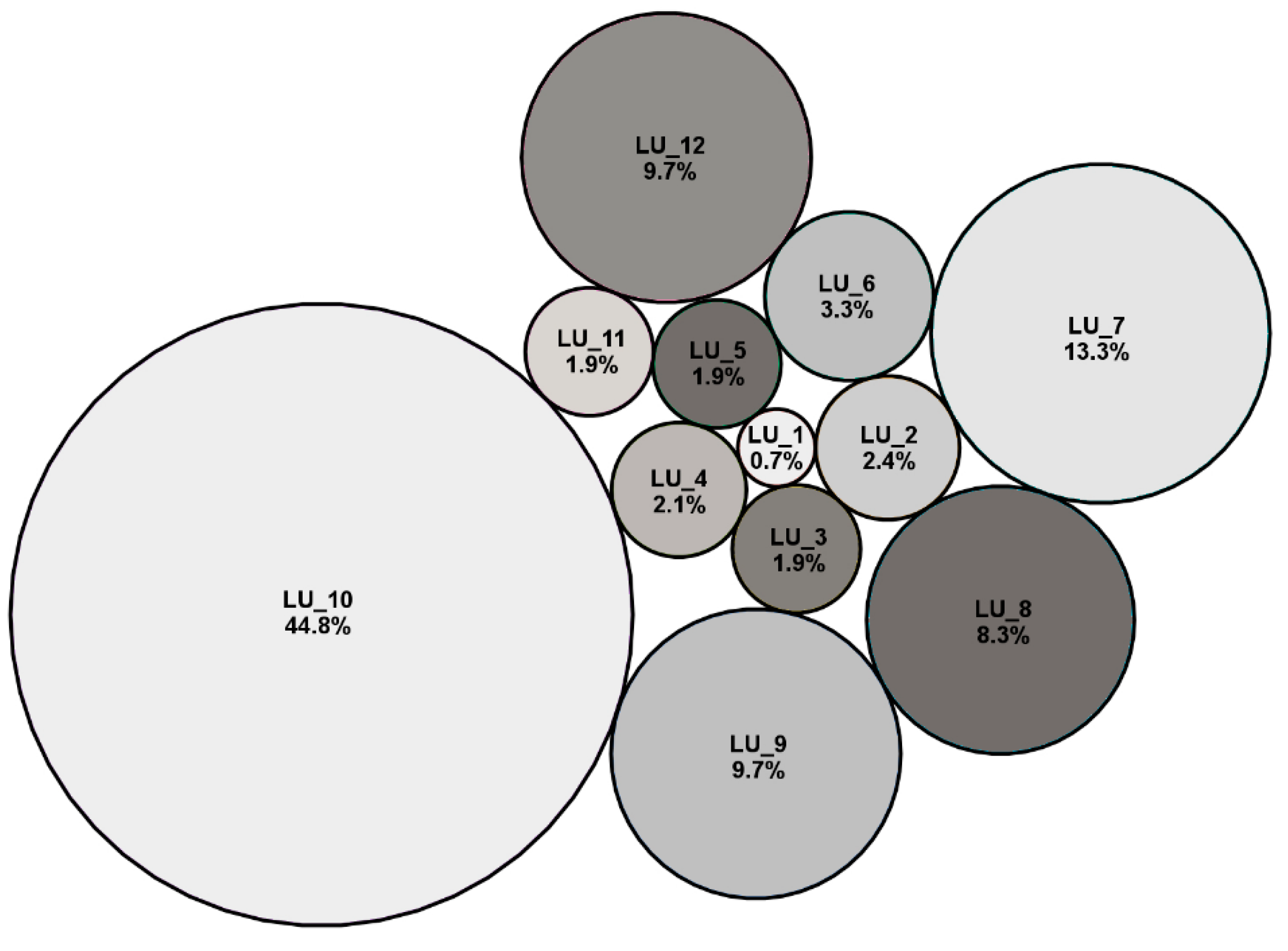
4.1. Land Use Classification

Land use is one of the elements constituting the landscape of a place. Based on land use, in the 1000 m buffer, using Ward’s hierarchical clustering and the Euclidean distance measure, a tree diagram with grouping for the sections of analyzed road was obtained (Figure A1). Based on the above-mentioned cluster analysis, twelve clusters of land use, characterized by different percentages of particular types of land use, were distinguished:

• LU_1—grasslands with surface water,
• LU_2—grasslands with built-up areas,
• LU_3—grasslands,
• LU_4—grasslands with arable lands,
• LU_5—forest areas and shrubs with grasslands,
• LU_6—forest areas and shrubs with arable lands,
• LU_7—forest areas and shrubs,
• LU_8—arable lands with forest areas and shrubs,
• LU_9—arable lands with grasslands,
• LU_10—arable lands,
• LU_11—arable lands with forest areas and shrubs and grasslands,
• LU_12—arable lands with grasslands and built-up areas.

The highest percentages of sections of road were classified in the arable lands cluster (LU_10: 44.8%) and forest areas and shrubs cluster (LU_7: 13.3%). The number of sections related to built-up areas was smaller (LU_2 and LU_12) (Figure 2).

4.2. Buffer Analysis

Based on Spearman’s rank correlation coefficient and the criterion of a very strong relationship between the analyzed data (|r| ≥ 0.9), three out of twelve landscape metrics were excluded from further analyses. They were characterized by a very strong level of correlation both with each other and with other metrics (

Table 2. Spearman’s rank correlation coefficient between landscape metrics.

		1	2	3	4	5	6	7	8	9
1	NP	1.00
2	PD	0.95 *	1.00
3	ED	0.91 *	0.93 *	1.00
4	LSI	0.93 *	0.91 *	0.99 *	1.00
5	AREA_MN	−0.95 *	−1.00 *	−0.93 *	−0.91 *	1.00
6	SHAPE_MN	−0.51 *	−0.51 *	−0.31 *	−0.30 *	0.51 *	1.00
7	PR	0.73 *	0.68 *	0.65 *	0.66 *	−0.68 *	−0.39 *	1.00
8	SHDI	0.78 *	0.78 *	0.88 *	0.88 *	−0.78 *	−0.34 *	0.60 *	1.00
9	SIEI	0.69 *	0.69 *	0.82 *	0.81 *	−0.69 *	−0.28 *	0.46 *	0.97 *	1.00

where: *—p ≤ 0.05; red color—|r| ≥ 0.9.

). Moreover, the elimination of metrics took into account the group to which the metrics belong (area and edge metrics, shape metrics, aggregation metrics and diversity metrics), so that at least one metric represents a different aspect of the measured landscape pattern. Excluded landscape metrics included the number of patches (NP), edge density (ED) and landscape shape index (LSI).

The results for the buffer analysis in designated land use clusters for the road indicate that the landscape structure was characterized by the smallest mean patch size (AREA_MN) close to the road, in 100 m buffer zones. For the analyzed road and the majority of land use clusters, a slight increase in the value of the landscape metric was observed with increasing distance from the road axis. However, based on the Mann–Kendall test, a statistically significant monotonic upward trend was found for the entire road and in the following clusters: grasslands with built-up areas (LU_2), forest areas and shrubs with arable lands (LU_6), forest areas and shrubs (LU_7), arable lands with forest areas and shrubs (LU_8) and arable lands with forest areas and shrubs and grasslands (LU_11) (

Table 3. Buffer analysis and Mann–Kendall test for mean patch size (AREA_MN) for the entire road and in designated land use clusters (mean ± standard error).

Cluster	Buffer Width [m]					Trend
	100	200	500	700	1000
Road	1.993 ± 0.048	3.393 ± 0.096	5.988 ± 0.224	6.770 ± 0.278	7.285 ± 0.350	↑
LU_1	1.078 ± 0.338	1.491 ± 0.511	1.917 ± 0.546	1.905 ± 0.403	1.999 ± 0.400
LU_2	0.956 ± 0.074	1.180 ± 0.108	1.473 ± 0.156	1.559 ± 0.137	1.612 ± 0.137	↑
LU_3	1.839 ± 0.600	2.816 ± 0.905	3.534 ± 0.980	3.131 ± 0.339	3.689 ± 0.704
LU_4	1.418 ± 0.261	2.286 ± 0.583	2.172 ± 0.355	2.247 ± 0.273	2.519 ± 0.302
LU_5	1.458 ± 0.335	2.255 ± 0.549	2.576 ± 0.561	2.532 ± 0.477	2.989 ± 0.642
LU_6	1.674 ± 0.198	2.518 ± 0.369	3.876 ± 0.500	4.373 ± 0.505	4.590 ± 0.581	↑
LU_7	2.468 ± 0.111	4.956 ± 0.237	10.775 ± 0.632	13.662 ± 0.902	17.213 ± 1.373	↑
LU_8	1.997 ± 0.166	3.071 ± 0.279	5.189 ± 0.527	6.336 ± 0.719	7.411 ± 0.907	↑
LU_9	1.552 ± 0.099	2.141 ± 0.153	2.847 ± 0.338	2.686 ± 0.234	2.648 ± 0.176
LU_10	2.236 ± 0.068	3.941 ± 0.133	7.206 ± 0.327	7.889 ± 0.376	7.710 ± 0.418
LU_11	1.135 ± 0.107	1.789 ± 0.218	2.546 ± 0.326	2.772 ± 0.276	2.782 ± 0.274	↑
LU_12	1.522 ± 0.162	2.136 ± 0.283	2.431 ± 0.225	2.406 ± 0.214	2.449 ± 0.187

where: ↑—statistically significant monotonic upward trend; empty field—no statistically significant monotonic trend.

).

The analysis of the results for mean shape index (SHAPE_MN) showed that the patches for the road and in all land use clusters had an irregular character and, with distance from the road axis, the shape became more regular—close to a circle or square—but the landscape metric did not reach 1.0 in any cluster. A monotonic downward trend was observed in most land use clusters, except the following clusters: grasslands with surface water (LU_1), grasslands with built-up areas (LU_2), grasslands (LU_3) and forest areas and shrubs with grasslands (LU_5) (

Table 4. Buffer analysis and the Mann–Kendall test for mean shape index (SHAPE_MN) for the entire road and in designated land use clusters (mean ± standard error).

Cluster	Buffer Width [m]					Trend
	100	200	500	700	1000
Road	2.460 ± 0.029	2.313 ± 0.026	2.149 ± 0.023	2.074 ± 0.021	1.987 ± 0.018	↓
LU_1	1.959 ± 0.274	1.821 ± 0.199	1.695 ± 0.097	1.697 ± 0.071	1.673 ± 0.036
LU_2	1.887 ± 0.032	1.850 ± 0.038	1.888 ± 0.024	1.870 ± 0.009	1.871 ± 0.018
LU_3	2.059 ± 0.166	1.894 ± 0.078	1.960 ± 0.069	1.924 ± 0.108	1.957 ± 0.058
LU_4	1.944 ± 0.076	1.859 ± 0.063	1.776 ± 0.058	1.770 ± 0.049	1.742 ± 0.046	↓
LU_5	2.027 ± 0.109	2.013 ± 0.099	1.870 ± 0.073	1.845 ± 0.063	1.891 ± 0.051
LU_6	2.347 ± 0.113	2.135 ± 0.071	1.996 ± 0.058	1.939 ± 0.048	1.848 ± 0.035	↓
LU_7	2.892 ± 0.089	2.845 ± 0.089	2.651 ± 0.080	2.575 ± 0.079	2.480 ± 0.079	↓
LU_8	2.503 ± 0.111	2.292 ± 0.070	2.108 ± 0.056	2.077 ± 0.051	2.022 ± 0.046	↓
LU_9	2.156 ± 0.066	1.998 ± 0.053	1.903 ± 0.047	1.825 ± 0.028	1.789 ± 0.023	↓
LU_10	2.600 ± 0.041	2.425 ± 0.036	2.206 ± 0.033	2.093 ± 0.029	1.951 ± 0.022	↓
LU_11	2.100 ± 0.058	1.982 ± 0.037	1.924 ± 0.043	1.916 ± 0.064	1.907 ± 0.038	↓
LU_12	2.058 ± 0.060	1.918 ± 0.042	1.847 ± 0.026	1.845 ± 0.023	1.835 ± 0.023	↓

where: ↓—statistically significant monotonic downward trend; empty field—no statistically significant monotonic trend.

).

The results obtained for patch density (PD) show that the number of patches per 100 hectares decreased with increasing distance from the road axis. For the entire road and in all land use clusters, except for the arable lands cluster (LU_10), a monotonic downward trend was revealed. The highest value of the landscape metric was observed in the grasslands with built-up areas cluster (LU_2), while the smallest was observed in the forest areas and shrubs cluster (LU_7) (

Table 5. Buffer analysis and the Mann–Kendall test for patch density (PD) for the entire road and in designated land use clusters (mean ± standard error).

Cluster	Buffer Width [m]					Trend
	100	200	500	700	1000
Road	63.597 ± 1.559	41.745 ± 1.254	29.301 ± 1.060	27.481 ± 1.004	26.273 ± 0.921	↓
LU_1	99.252 ± 28.535	81.310 ± 20.781	60.783 ± 15.641	57.211 ± 11.399	54.001 ± 10.116	↓
LU_2	99.226 ± 9.871	90.649 ± 7.541	74.627 ± 7.369	68.216 ± 5.315	65.578 ± 4.742	↓
LU_3	86.439 ± 15.312	59.268 ± 11.869	39.422 ± 6.859	35.584 ± 4.922	33.235 ± 5.314	↓
LU_4	87.228 ± 11.871	64.274 ± 10.926	55.518 ± 7.662	50.366 ± 6.312	44.754 ± 5.465	↓
LU_5	87.820 ± 13.838	61.943 ± 11.722	51.143 ± 9.521	48.922 ± 8.237	43.309 ± 7.934	↓
LU_6	69.248 ± 6.907	45.609 ± 3.544	30.992 ± 3.478	27.428 ± 3.186	26.467 ± 3.055	↓
LU_7	46.082 ± 2.402	23.798 ± 1.460	12.047 ± 0.941	10.293 ± 0.974	9.088 ± 0.911	↓
LU_8	63.717 ± 5.217	41.552 ± 3.237	26.131 ± 2.389	23.849 ± 2.835	20.189 ± 1.946	↓
LU_9	75.795 ± 5.085	56.227 ± 3.669	45.667 ± 2.912	44.767 ± 2.566	42.519 ± 1.988	↓
LU_10	52.934 ± 1.681	31.662 ± 1.167	20.095 ± 0.905	18.720 ± 0.840	18.874 ± 0.754
LU_11	94.411 ± 9.887	60.906 ± 6.153	43.756 ± 5.338	39.015 ± 4.309	38.232 ± 3.367	↓
LU_12	87.033 ± 5.980	66.235 ± 4.993	52.893 ± 3.669	52.029 ± 3.376	50.051 ± 3.310	↓

where: ↓—statistically significant monotonic downward trend; empty field—no statistically significant monotonic trend.

).

The analysis of patch richness (PR) for the road indicated that the most different patch types per section were observed in the grasslands with surface water cluster (LU_1), as well as the grasslands with built-up areas cluster (LU_2). The smallest number of patch types was found in the grasslands cluster (LU_3), forest areas and shrubs cluster (LU_7) and arable lands cluster (LU_10). Based on the results of the Mann–Kendall test, a monotonic upward trend in all clusters was detected (

Table 6. Buffer analysis and the Mann–Kendall test for patch richness (PR) for the entire road and in designated land use clusters (mean ± standard error).

Cluster	Buffer Width [m]					Trend
	100	200	500	700	1000
Road	4.118 ± 0.052	4.517 ± 0.059	5.178 ± 0.066	5.533 ± 0.067	6.005 ± 0.066	↑
LU_1	4.667 ± 0.333	5.667 ± 0.882	6.667 ± 0.667	7.000 ± 0.577	7.000 ± 0.577	↑
LU_2	5.400 ± 0.306	6.200 ± 0.249	7.000 ± 0.211	7.400 ± 0.163	7.500 ± 0.167	↑
LU_3	3.875 ± 0.515	4.250 ± 0.559	4.750 ± 0.453	5.000 ± 0.535	5.625 ± 0.324	↑
LU_4	4.667 ± 0.333	5.111 ± 0.423	5.667 ± 0.289	6.000 ± 0.167	6.111 ± 0.111	↑
LU_5	4.375 ± 0.375	4.750 ± 0.366	5.875 ± 0.227	6.625 ± 0.375	6.750 ± 0.453	↑
LU_6	4.571 ± 0.251	5.071 ± 0.221	5.500 ± 0.272	5.786 ± 0.239	6.286 ± 0.304	↑
LU_7	3.589 ± 0.101	3.696 ± 0.119	3.911 ± 0.147	4.107 ± 0.163	4.357 ± 0.177	↑
LU_8	4.229 ± 0.179	4.771 ± 0.179	5.314 ± 0.157	5.457 ± 0.161	5.800 ± 0.158	↑
LU_9	4.512 ± 0.160	5.146 ± 0.150	6.171 ± 0.160	6.537 ± 0.140	6.854 ± 0.119	↑
LU_10	3.884 ± 0.069	4.212 ± 0.079	4.921 ± 0.095	5.344 ± 0.093	6.000 ± 0.089	↑
LU_11	4.250 ± 0.313	4.875 ± 0.227	5.750 ± 0.313	5.750 ± 0.313	6.125 ± 0.295	↑
LU_12	4.780 ± 0.202	5.317 ± 0.208	6.049 ± 0.164	6.512 ± 0.161	6.915 ± 0.152	↑

where: ↑—statistically significant monotonic upward trend; empty field—no statistically significant monotonic trend.

).

The values of Shannon’s diversity index (SHDI) for the entire road, forest areas and shrubs cluster (LU_7) and arable lands cluster (LU_10) decreased with increasing distance from the road axis. This was confirmed by the Mann–Kendall test, which for these clusters showed a monotonic downward trend. For the grasslands with surface water cluster (LU_1), grasslands with built-up areas cluster (LU_2) and forest areas and shrubs with grasslands cluster (LU_5), an increasing tendency was observed. However, only in the case of the forest areas and shrubs with grasslands cluster (LU_5) was this tendency a statistically significant monotonic upward trend. For the other clusters, the values of the landscape metric changed slightly depending on the distance from the road axis (

Table 7. Buffer analysis and the Mann–Kendall test for Shannon’s diversity index (SHDI) for the entire road and in designated land use clusters (mean ± standard error).

Cluster	Buffer Width [m]					Trend
	100	200	500	700	1000
Road	1.070 ± 0.010	0.968 ± 0.014	0.842 ± 0.018	0.822 ± 0.019	0.822 ± 0.019	↓
LU_1	1.272 ± 0.055	1.392 ± 0.114	1.469 ± 0.182	1.451 ± 0.165	1.457 ± 0.137
LU_2	1.173 ± 0.050	1.330 ± 0.051	1.416 ± 0.047	1.414 ± 0.045	1.443 ± 0.063
LU_3	0.877 ± 0.083	0.871 ± 0.127	0.767 ± 0.112	0.751 ± 0.107	0.793 ± 0.097
LU_4	1.097 ± 0.063	1.129 ± 0.089	1.123 ± 0.078	1.169 ± 0.062	1.209 ± 0.052
LU_5	1.116 ± 0.062	1.191 ± 0.068	1.265 ± 0.045	1.299 ± 0.061	1.334 ± 0.073	↑
LU_6	1.096 ± 0.063	1.040 ± 0.077	1.057 ± 0.081	1.066 ± 0.059	1.082 ± 0.059
LU_7	1.008 ± 0.021	0.785 ± 0.029	0.520 ± 0.029	0.463 ± 0.029	0.433 ± 0.030	↓
LU_8	1.154 ± 0.042	1.101 ± 0.050	1.043 ± 0.036	1.042 ± 0.029	1.042 ± 0.026
LU_9	1.160 ± 0.036	1.163 ± 0.043	1.186 ± 0.037	1.184 ± 0.029	1.185 ± 0.016
LU_10	1.026 ± 0.014	0.851 ± 0.017	0.642 ± 0.019	0.599 ± 0.019	0.594 ± 0.017	↓
LU_11	1.225 ± 0.046	1.245 ± 0.055	1.293 ± 0.032	1.302 ± 0.023	1.318 ± 0.021
LU_12	1.135 ± 0.036	1.188 ± 0.046	1.213 ± 0.036	1.263 ± 0.031	1.294 ± 0.027

where: ↑—statistically significant monotonic upward trend; ↓—statistically significant monotonic downward trend; empty field—no statistically significant monotonic trend.

).

The results for Simpson’s evenness index (SIEI) revealed that the most even spatial distribution between types of patches was in the 100 m buffer zone. For the road and in the majority of sections, the value of the metric decreased with the distance from the road axis, which indicated an increasingly uneven distribution between patches. However, based on results of the Mann–Kendall test, a monotonic downward trend in the following clusters was detected: forest areas and shrubs (LU_7), arable lands with grasslands (LU_9), arable lands (LU_10) and arable lands with grasslands and built-up areas (LU_12) (

Table 8. Buffer analysis and the Mann–Kendall test for Simpson’s evenness index (SIEI) for the entire road and in designated land use clusters (mean ± standard error).

Cluster	Buffer Width [m]					Trend
	100	200	500	700	1000
Road	0.815 ± 0.005	0.669 ± 0.008	0.525 ± 0.011	0.499 ± 0.012	0.487 ± 0.012	↓
LU_1	0.856 ± 0.012	0.863 ± 0.020	0.840 ± 0.057	0.831 ± 0.055	0.837 ± 0.045
LU_2	0.770 ± 0.036	0.805 ± 0.030	0.811 ± 0.021	0.800 ± 0.019	0.800 ± 0.026
LU_3	0.757 ± 0.045	0.624 ± 0.051	0.470 ± 0.059	0.449 ± 0.057	0.456 ± 0.057
LU_4	0.796 ± 0.030	0.755 ± 0.050	0.692 ± 0.046	0.700 ± 0.039	0.741 ± 0.024
LU_5	0.821 ± 0.027	0.822 ± 0.041	0.796 ± 0.027	0.797 ± 0.025	0.809 ± 0.027
LU_6	0.778 ± 0.026	0.671 ± 0.047	0.667 ± 0.049	0.678 ± 0.032	0.683 ± 0.024
LU_7	0.813 ± 0.012	0.588 ± 0.020	0.346 ± 0.020	0.295 ± 0.019	0.266 ± 0.020	↓
LU_8	0.839 ± 0.022	0.735 ± 0.031	0.687 ± 0.023	0.694 ± 0.018	0.697 ± 0.014
LU_9	0.838 ± 0.014	0.764 ± 0.022	0.719 ± 0.021	0.710 ± 0.016	0.699 ± 0.007	↓
LU_10	0.809 ± 0.008	0.610 ± 0.010	0.397 ± 0.012	0.350 ± 0.012	0.329 ± 0.011	↓
LU_11	0.916 ± 0.020	0.856 ± 0.012	0.838 ± 0.013	0.850 ± 0.008	0.841 ± 0.005
LU_12	0.816 ± 0.012	0.775 ± 0.020	0.746 ± 0.017	0.769 ± 0.011	0.777 ± 0.009	↓

where: ↓—statistically significant monotonic downward trend; empty field—no statistically significant monotonic trend.

).

4.3. Change Point

The identification of changes in the mean and variance using the “at most one change” (AMOC) method indicated different change points for the analyzed landscape metrics and land use clusters. The spatial distribution of change points for all landscape metrics was heterogeneous (Figure 3).

The AMOC method for mean patch size (AREA_MN) revealed the occurrence of a change point in the entire road and in designated land use clusters, with the exception of grasslands with surface water (LU_1). For the road, the change point was observed over a 700 m buffer zone, whereas for most land use clusters, a significant change in the value of the metric was observed after a buffer width of 200 m. In the forest areas and shrubs with arable lands cluster (LU_6), the change point was detected after a 500 m buffer, and for the forest areas and shrubs cluster (LU_7) and the arable lands with forest areas and shrubs cluster (LU_8), after 700 m. The analysis for the mean shape index (SHAPE_MN) showed a significant change in the value of the metric after a 200 m buffer for such land use clusters as grasslands (LU_3), forest areas and shrubs with grasslands (LU_5), forest areas and shrubs with arable lands (LU_6), arable lands with grasslands (LU_9), arable lands (LU_10), arable lands with forest areas and shrubs and grasslands (LU_11), and arable lands with grasslands and built-up areas (LU_12). On the basis of the results of AMOC for patch density (PD), a change point was observed in all the analyzed land use clusters. A significant change point after a 700 m buffer was observed for the road and the majority of land use clusters. In the case of the grasslands with surface water cluster (LU_1), as well as arable lands (LU_10), the change point was different: 200 m and 500 m buffers, respectively. The change point in the 500 m buffer was observed in the road and in the majority of clusters for patch richness (PR). For the LU_2 (grasslands with built-up areas), LU_8 (arable lands with forest areas and shrubs), LU_9 (arable lands with grasslands), LU_11 (arable lands with forest areas and shrubs and grasslands) and LU_12 (arable lands with grasslands and built-up areas) clusters, the change point was found after a buffer of 200 m. For the LU_6 (forest areas and shrubs with arable lands) and LU_10 (arable lands) clusters, the analysis showed a change in the metric over a 700 m buffer. Based on the AMOC method for Shannon’s diversity index (SHDI), the change point in the 200 m buffer was observed in the entire road and in two clusters: LU_7 (forest areas and shrubs) and LU_10 (arable lands). The analysis for Simpson’s evenness index (SIEI) indicated the change point only for the entire road (

Table 9. Identification of changes in the mean and variance using the “at most one change” (AMOC) method for landscape metrics for the entire road and in designated land use clusters.

Cluster	AREA_MN	SHAPE_MN	PD	PR	SHDI	SIEI
Road	700	–	700	500	200	100
LU_1	–	–	200	500	–	–
LU_2	200	–	700	200	–	–
LU_3	200	200	700	500	–	–
LU_4	200	–	700	500	–	–
LU_5	200	200	700	500	–	–
LU_6	500	200	700	700	–	–
LU_7	700	–	700	500	200	–
LU_8	700	–	700	200	–	–
LU_9	200	200	700	200	–	–
LU_10	200	200	500	700	200	–
LU_11	200	200	700	200	–	–
LU_12	200	200	700	200	–	–

where: – no changes in the mean and variance.

).

5. Discussion

The land use analyses showed that arable land and forest areas and shrubs dominated along the highway. There was also a relatively large number of built-up areas. These types of land use have been common for areas along roads [9,12,22,59,60,61]. According to Liang et al. [60], roads have been much more connected with areas transformed by human activities than with natural types of land cover, which in turn determines different, local patterns of landscape structures.

The highest value of mean patch size (AREA_MN) was observed for road sections classified as forest areas and shrubs, whereas the lowest value was observed for grasslands with built-up areas. The conducted analyses revealed that the smallest value of the metric occurred near the highway (100 m buffer). According to previous studies, low values of the metrics describing the area and edge of the patches indicated the fragmentation of the landscape related to the development of the road network [43,46,62]. The metric describing the shape of the patches—mean shape index (SHAPE_MN)—showed that the patches in all clusters were irregular, but for most of them, the shape became more regular after the 200 m buffer zone. According to Saunders et al. [43], it may suggest a landscape more transformed by human activity. However, Su et al. [13] and Song et al. [45] stated that high values of SHAPE_MN may also be related to human disturbance of the landscape and this is the indirect impact of roads. The results obtained for patch density (PD) indicated that the number of patches per 100 hectares for the road and clusters usually decreased with the distance from the road axis. Liu et al. [12] and Su et al. [13] also observed this trend for different types of roads, in contrast to Song et al. [45], who noted higher values of the metrics near roads. In the present study, the highest values of patch density were observed for sections associated with grasslands and surface water, as well as grasslands and built-up areas. The results for two diversity metrics—patch richness (PR) and Shannon’s diversity index (SHDI)—indicated similar trends depending on the distance from the road axis. A different tendency was observed for Simpson’s evenness index (SIEI), which may be related to the characteristics of this metric. As pointed out by McGarigal and Marks [42] and McGarigal [63], SHDI is more sensitive to the occurrence of rare types of land use, while SIEI is more easily influenced by dominant types. The increasing number of patch types with increasing distance from the road axis was observed for patch richness (PR). The largest number of different patches was observed in clusters related to grasslands and surface water, as well as grasslands and built-up areas, while the lowest was observed in forest areas and shrubs. Roo-Zielińska et al. [59] and Wu et al. [22] also found different landscape structures for forest and built-up areas. In addition, it was pointed out that built-up areas were most often located near surface waters, which may explain the obtained high value of PR for the cluster associated with surface water. The analysis of Shannon’s diversity index (SHDI) showed a significant downward trend for clusters classified as forest and shrub vegetation, as well as arable land. Sections from these clusters were also characterized by the lowest metric value. An upward tendency of SHDI was observed in the majority of other land use clusters, whereas Liu et al. [12] and Su et al. [13] reported the existence of a downward trend for all examined roads. However, in those investigations, the analyzed roads were surrounded mainly by forests and arable lands, for which a downward trend was also detected in our research. The change point for the studied road was observed only for the entire road and the two following clusters: forest areas and shrubs, as well as arable lands. For other clusters, no change point was found in the analyzed buffer ranges, which is confirmed by the results of Su et al. [13]. The results observed for Simpson’s evenness index (SIEI) show that the most even spatial distribution between patch types was near the road. The SIEI value decreased with the increasing distance from the road axis, similarly to Liu et al. [12] and Su et al. [13]. The change point was affirmed only for the entire road in the 100 m buffer zone. By contrast to the whole road, there was no occurrence of a change point in the metric value for all land use clusters in the analyzed buffer ranges, which was also observed by Su et al. [13].

Although the present research has provided new results and insights, some potential limitations should be noted. The first limitation concerns the input data. The land use data from official repositories or remote sensing data are often used. In both cases, the problem is to define landscape elements and land use classes that depend on the purpose of the study [64]. Secondly, landscape metrics are calculated on the basis of cartographic data; hence, the thematic and geometric resolution influences the results of the analyses. Scale is also crucial because most landscape metrics are sensitive to grain and extent [42,64]. In addition, landscape metrics can react unpredictably to thematic or temporal changes [59]. It should also be emphasized that, with landscape metrics, only planimetric areas and distances are calculated. It is a simplification of reality, since relief is not taken into account [64,65]. Another limitation concerns the class of road. The undertaken research analyzed only the impact of a highway, whereas previous research indicated that the road-effect zone was wider for a highway in comparison to the road-effect zone for provincial or rural roads [12,13].

6. Conclusions

The results obtained for the landscape metrics indicate the negative impact of roads on the landscape structure. Based on our results, it could be concluded that, due to changes of values of metrics in the buffer analysis, the investigated road contributed to an increase in fragmentation, decrease in diversity of the landscape and an increased domination of one type of land use near roads.

The values of the landscape metrics, depending on the distance from the road axis, revealed spatial diversity in the landscape structure; hence, they can be helpful in assessing the impact of road investments on the landscape. Nevertheless, it should be remembered that landscape metrics have been calculated equally for all types of land use, irrespective of their natural and landscape value. However, taking into account the change point for particular landscape metrics, the range of impact was different for the road as a whole and for land use clusters. Therefore, to analyze the road-effect zone, it is necessary to take into account not only different ranges of impact according to the type of road or the time of exploitation, but also the different types of land use of areas surrounding the road. The results of the present study might be especially valuable for further recommendations during the environmental impact assessments of new constructed highways, as well as for the sustainable development of areas around roads. This is especially valid in view of the lack of a proper methodology to analyze the effect of roads on the landscape structure. Our investigations partially filled this gap, but it is still necessary to conduct a detailed analysis of different road classes and various relief forms.

References

1. Forman, R.T. Estimate of the area affected ecologically by the road system in the United States. Conserv. Biol. 2000, 14, 31–35. [Google Scholar] [CrossRef]
2. Forman, R.T.; Deblinger, R.D. The ecological road-effect zone of a Massachusetts (USA) suburban highway. Conserv. Biol. 2000, 14, 36–46. [Google Scholar] [CrossRef]
3. Morawska, A.; Żelazo, J. Oddziaływanie dróg na środowisko i rola postępowania w sprawie OOS na przykładzie planowanej drogi krajowej. Przegląd Naukowy. Inżynieria i Kształtowanie Środowiska 2008, 4, 95–100. [Google Scholar]
4. Lin, S.-C. The width of edge effects of road construction on fauna and ecologically critical road density. J. Environ. Eng. Landsc. 2015, 23, 241–250. [Google Scholar] [CrossRef] [Green Version]
5. Karlson, M.; Mörtberg, U.; Balfors, B. Road ecology in environmental impact assessment. Environ. Impact Asses. 2014, 48, 10–19. [Google Scholar] [CrossRef]
6. Khanani, R.S.; Adugbila, E.J.; Martinez, J.A.; Pfeffer, K. The Impact of Road Infrastructure Development Projects on Local Communities in Peri-Urban Areas: The Case of Kisumu, Kenya and Accra, Ghana. Int. J. Community Well-Being 2020, 4, 1–21. [Google Scholar] [CrossRef]
7. National Research Council (NRC). Assessing and Managing the Ecological Impacts of Paved Roads; Committee on Ecological Impacts of Road Density, National Academies Press: Washington, DC, USA, 2005; pp. 1–294. [Google Scholar]
8. Komornicki, T.; Wiśniewski, R.; Baranowski, J.; Błażejczyk, K.; Degórski, M.; Goliszek, S.; Rosik, P.; Solon, J.; Stępniak, M.; Zawiska, I. Wpływ Wybranych Korytarzy Drogowych na Srodowisko Przyrodnicze i Rozwój Społeczno-Ekonomiczny Obszarów Przyległych; Instytut Geografii i Przestrzennego Zagospodarowania PAN im. Stanisława Leszczyckiego: Warszawa, Poland, 2015; Volume 249, pp. 115–118. [Google Scholar]
9. Hawbaker, T.J.; Radeloff, V.C. Roads and landscape pattern in northern Wisconsin based on a comparison of four road data sources. Conserv. Biol. 2004, 18, 1233–1244. [Google Scholar] [CrossRef]
10. Forman, R.T. Land Mosaics: The Ecology of Landscapes and Regions; Cambridge University Press: Cambridge, UK, 1995; pp. 1–623. [Google Scholar]
11. Igondova, E.; Pavlickova, K.; Majzlan, O. The ecological impact assessment of a proposed road development (the Slovak approach). Environ. Impact Assess. 2016, 59, 43–54. [Google Scholar] [CrossRef]
12. Liu, S.L.; Cui, B.S.; Dong, S.K.; Yang, Z.F.; Yang, M.; Holt, K. Evaluating the influence of road networks on landscape and regional ecological risk—A case study in Lancang River Valley of Southwest China. Ecol. Eng. 2008, 34, 91–99. [Google Scholar] [CrossRef]
13. Su, S.; Xiao, R.; Li, D. Impacts of transportation routes on landscape diversity: A comparison of different route types and their combined effects. Environ. Manag. 2014, 53, 636–647. [Google Scholar] [CrossRef]
14. Reijnen, R.; Foppen, R.; Braak, C.T.; Thissen, J. The effects of car traffic on breeding bird populations in woodland. III. Reduction of density in relation to the proximity of main roads. J. Appl. Ecol. 1995, 32, 187–202. [Google Scholar] [CrossRef]
15. Semlitsch, R.D.; Ryan, T.J.; Hamed, K.; Chatfield, M.; Drehman, B.; Pekarek, N.; Spath, M.; Watland, A. Salamander abundance along road edges and within abandoned logging roads in Appalachian forests. Conserv. Biol. 2007, 21, 159–167. [Google Scholar] [CrossRef] [PubMed] [Green Version]
16. Eigenbrod, F.; Hecnar, S.J.; Fahrig, L. Quantifying the road-effect zone: Threshold effects of a motorway on anuran populations in Ontario, Canada. Ecol. Soc. 2009, 14, 24. [Google Scholar] [CrossRef] [Green Version]
17. Torres, A.A.; Palacín, C.; Seoane, J.; Alonso, J.C. Assessing the effects of a highway on a threatened species using Before-During-After and Before-During- After-Control-Impact designs. Biol. Conserv. 2011, 144, 2223–2232. [Google Scholar] [CrossRef]
18. He, K.; Dai, Q.; Gu, X.; Zhang, Z.; Zhou, J.; Qi, D.; Yang, X.; Zhang, W.; Yang, B.; Yang, Z. Effects of roads on giant panda distribution: A mountain range scale evaluation. Sci. Rep. 2019, 9, 1110. [Google Scholar] [CrossRef] [Green Version]
19. Medinas, D.; Ribeiro, V.; Marques, J.T.; Silva, B.; Barbosa, A.M.; Rebelo, H.; Mira, A. Road effects on bat activity depend on surrounding habitat type. Sci. Total Environ. 2019, 660, 340–347. [Google Scholar] [CrossRef]
20. Boarman, W.I.; Sazaki, M. A highway’s road-effect zone for desert tortoises (Gopherus agassizii). J. Arid Environ. 2006, 65, 94–101. [Google Scholar] [CrossRef]
21. Deljouei, A.; Sadeghi, S.M.M.; Abdi, E.; Bernhardt-Römermann, M.; Pascoe, E.L.; Marcantonio, M. The impact of road disturbance on vegetation and soil properties in a beech stand, Hyrcanian forest. Eur. J. Forest Res. 2018, 137, 759–770. [Google Scholar] [CrossRef]
22. Wu, C.F.; Lin, Y.P.; Chiang, L.C.; Huang, T. Assessing highway’s impacts on landscape patterns and ecosystem services: A case study in Puli Township, Taiwan. Landscape Urban Plan. 2014, 128, 60–71. [Google Scholar] [CrossRef]
23. Fiedeń, Ł. Changes in land use in the communes crossed by the A4 motorway in Poland. Land Use Policy 2019, 85, 397–406. [Google Scholar] [CrossRef]
24. Wang, J.; Cui, B.; Liu, S.; Dong, S.; Wei, G.; Liu, J. Effects of road networks on ecosystem service value in the longitudinal range-gorge region. Chin. Sci. Bull. 2007, 52, 180–191. [Google Scholar] [CrossRef]
25. Ying, L.; Shen, Z.; Chen, J.; Fang, R.; Chen, X.; Jiang, R. Spatiotemporal patterns of road network and road development priority in Three Parallel Rivers Region in Yunnan, China: An evaluation based on modified kernel distance estimate. Chin. Geogr. Sci. 2014, 24, 39–49. [Google Scholar] [CrossRef] [Green Version]
26. Nita, J.; Myga-Piątek, U. Ocena walorów widokowych drogi S1 [E75] na odcinku Częstochowa-Sosnowiec. Pr. Kom. Kraj. Kult. 2012, 18, 181–193. [Google Scholar]
27. Sas-Bojarska, A. Nowe wyzwania dla architektury krajobrazu-oceny środowiskowe, Czasopismo Techniczne. Architektura 2007, 104, 83–85. [Google Scholar]
28. Sas-Bojarska, A. Wielkie Inwestycje W Kontekście Zagrożeń I Ochrony Krajobrazu; Wydawnictwo Politechniki Gdańskiej: Gdańsk, Poland, 2007; pp. 1–224. [Google Scholar]
29. Forczek-Brataniec, U. Widok z Drogi: Krajobraz w Percepcji Dynamicznej; Wydawnictwo Elamed: Katowice, Poland, 2008; pp. 1–184. [Google Scholar]
30. Forczek-Brataniec, U. Udział architekta krajobrazu w planowaniu widokowym tras komunikacyjnych na przykładzie studiów krajobrazowego przekroczenia Alei Solidarności w Nowej Hucie drogą ekspresową S7. Teka Kom. Archit. Urban. Studiów Kraj. PAN 2013, 9, 20–31. [Google Scholar]
31. Forczek-Brataniec, U. Nowa droga w krajobrazie. Archit. Kraj. 2013, 1/2013, 18–29. [Google Scholar]
32. Janeczko, E. Podstawy metodyczne oceny krajobrazu leśnego w otoczeniu szlaków komunikacyjnych. Probl. Ekol. Kraj. 2008, XX, 363–369. [Google Scholar]
33. Winiarski, W.; Janeczko, E. Ocena walorów krajobrazowych wybranych alei na terenie gminy Dubeninki. Rocz. Pol. Tow. Dendrol. 2011, 59, 77–84. [Google Scholar]
34. Nita, J.; Myga-Piątek, U. Scenic values of the Katowice-Częstochowa section of national road No. 1. Geogr. Pol. 2014, 87, 113–125. [Google Scholar] [CrossRef] [Green Version]
35. Pukowiec, K.; Pytel, S. Infrastruktura drogowa w krajobrazie w świetle opinii mieszkańców na przykładzie autostrady A1 (odcinek Świerklany-Gorzyczki). Pr. Kom. Kraj. Kult. 2012, 18, 160–170. [Google Scholar]
36. Łowicki, D. Ocena krajobrazu na potrzeby planowania przestrzennego w Aglomeracji Poznańskiej. Probl. Ekol. Kraj. 2014, XXXVIII, 125–134. [Google Scholar]
37. Łowicki, D. Walory widokowe dróg w aglomeracji poznańskiej—Przykład Parku Krajobrazowego Puszcza Zielonka. Biuletyn Parków Krajobrazowych Wielkopolski 2015, 21, 46–58. [Google Scholar]
38. Trzaskowska, E. Analiza wizualna krajobrazu przy głównych trasach wjazdowych do Lublina. Acta Sci. Pol. Adm. Locorum 2014, 13, 35–44. [Google Scholar]
39. Janeczko, E.; Janeczko, K.; Moskalik, T.; Woźnicka, M. Assessment of the forest landscape along selected motor vehicle routes. Folia For. Pol. 2016, 58, 43–51. [Google Scholar] [CrossRef] [Green Version]
40. Lisiak, M.; Borowiak, K.; Kanclerz, J.; Adamska, A.; Szymańczyk, J. Effect of linear investment on nature and landscape–a case study. J. Environ. Eng. Landsc. 2018, 26, 158–165. [Google Scholar] [CrossRef]
41. Autostrada Wielkopolska, S.A. Letter to K. Borowiak. Repository of Department of Ecology and Environmental Protection 2017 (AWSA/DT/EP/1050/2017).
42. McGarigal, K.; Marks, B.J. FRAGSTATS: Spatial Pattern Analysis Program for Quantifying Landscape Structure; US Department of Agriculture, Forest Service, Pacific Northwest Research Station: Corvallis, OR, USA, 1995; pp. 1–122. [Google Scholar]
43. Saunders, S.C.; Mislivets, M.R.; Chen, J.; Cleland, D.T. Effects of roads on landscape structure within nested ecological units of the Northern Great Lakes Region, USA. Biol. Conserv. 2002, 103, 209–225. [Google Scholar] [CrossRef]
44. Tian, G.; Wu, J. Comparing urbanization patterns in Guangzhou of China and Phoenix of the USA: The influences of roads and rivers. Ecol. Indic. 2015, 52, 23–30. [Google Scholar] [CrossRef]
45. Song, J.; Ye, J.; Zhu, E.; Deng, J.; Wang, K. Analyzing the impact of highways associated with farmland loss under rapid urbanization. ISPRS Int. J. Geo-Inf. 2016, 5, 94. [Google Scholar] [CrossRef] [Green Version]
46. McGarigal, K.; Romme, W.H.; Crist, M.; Roworth, E. Cumulative effects of roads and logging on landscape structure in the San Juan Mountains, Colorado (USA). Landsc. Ecol. 2001, 16, 327–349. [Google Scholar] [CrossRef]
47. Gao, Y.; Zeng, Z.; Pan, Y.; Zhao, C. The Influence of Highway on the Roadside Landscape Pattern Change of Land Use. In Proceedings of the Fourth International Symposium on Knowledge Acquisition and Modeling, Sanya, China, 8–9 October 2011; IEEE Computer Society: Washington, DC, USA, 2011; pp. 451–453. [Google Scholar] [CrossRef]
48. Liu, Y.; Wang, H.; Jiao, L.; Liu, Y.; He, J.; Ai, T. Road centrality and landscape spatial patterns in Wuhan Metropolitan Area, China. Chinese Geogr. Sci. 2015, 25, 511–522. [Google Scholar] [CrossRef]
49. Hosseini Vardei, M.; Salmanmahiny, A.; Monavari, S.M.; Kheirkhah Zarkesh, M.M. Cumulative effects of developed road network on woodland—A landscape approach. Environ. Monit. Assess. 2014, 186, 7335–7347. [Google Scholar] [CrossRef] [PubMed]
50. Reed, R.A.; Johnson-Barnard, J.; Baker, W.L. Contribution of roads to forest fragmentation in the Rocky Mountains. Conserv. Biol. 1996, 10, 1098–1106. [Google Scholar] [CrossRef]
51. Ward, J.H. Hierarchical grouping to optimize an objective function. J. Am. Stat. Assoc. 1963, 58, 236–244. [Google Scholar] [CrossRef]
52. Inkoom, J.N.; Frank, S.; Greve, K.; Walz, U.; Fürst, C. Suitability of different landscape metrics for the assessments of patchy landscapes in West Africa. Ecol. Indic. 2018, 85, 117–127. [Google Scholar] [CrossRef]
53. Riitters, K.H.; O’neill, R.V.; Hunsaker, C.T.; Wickham, J.D.; Yankee, D.H.; Timmins, S.P.; Jones, K.B.; Jackson, B.L. A factor analysis of landscape pattern and structure metrics. Landsc. Ecol. 1995, 10, 23–39. [Google Scholar] [CrossRef]
54. Hussain, M.; Mahmud, I. pyMannKendall: A python package for non parametric Mann Kendall family of trend tests. J. Open Source Softw. 2019, 4, 1556. [Google Scholar] [CrossRef]
55. Hipel, K.W.; McLeod, A.I. Time Series Modelling of Water Resources and Environmental Systems; Elsevier: Amsterdam, The Netherlands, 1994; Electronic reprint of book originally published in 1994; Available online: http://www.stats.uwo.ca/faculty/aim/1994Book/ (accessed on 16 October 2018).
56. Libiseller, C.; Grimvall, A. Performance of partial Mann–Kendall tests for trend detection in the presence of covariates. Environmetrics 2002, 13, 71–84. [Google Scholar] [CrossRef]
57. Chen, J.; Gupta, A.K. Parametric Statistical Change Point Analysis: With Applications to Genetics, Medicine, and Finance; Birkhäuser: Boston, MA, USA, 2000; pp. 1–273. [Google Scholar]
58. R Core Team. R: A Language and Environment for Statistical Computing; R Foundation for Statistical Computing: Vienna, Austria, 2014; Available online: http://www.R-project.org/ (accessed on 1 November 2020).
59. Roo-Zielińska, E.; Solon, J.; Degórski, M. Ocena Stanu i Przekształceń Srodowiska Przyrodniczego na Podstawie Wskaźników Geobotanicznych, Krajobrazowych i Glebowych (Podstawy Teoretyczne i Przykłady Zastosowań); PAN IGiPZ: Warsaw, Poland, 2007; pp. 1–67. [Google Scholar]
60. Liang, J.; Liu, Y.; Ying, L.; Li, P.; Xu, Y.; Shen, Z. Road impacts on spatial patterns of land use and landscape fragmentation in three parallel rivers region, Yunnan Province, China. Chin. Geogr. Sci. 2014, 24, 15–27. [Google Scholar] [CrossRef] [Green Version]
61. Mo, W.; Wang, Y.; Zhang, Y.; Zhuang, D. Impacts of road network expansion on landscape ecological risk in a megacity, China: A case study of Beijing. Sci. Total Environ. 2017, 574, 1000–1011. [Google Scholar] [CrossRef] [Green Version]
62. Jaeger, J.; Schwarz-von Raumer, H.G.; Esswein, H.; Müller, M.; Schmidt-Lüttmann, M. Time series of landscape fragmentation caused by transportation infrastructure and urban development: A case study from Baden-Württemberg, Germany. Eco. Soc. 2017, 12, 1–28. [Google Scholar] [CrossRef]
63. McGarigal, K. FRAGSTATS Help. Documentation for FRAGSTATS. Available online: https://www.umass.edu/landeco/research/fragstats/documents/fragstats.help.4.2.pdf (accessed on 16 October 2018).
64. Walz, U. Landscape structure, landscape metrics and biodiversity. Living Rev. Landsc. Res. 2011, 5, 1–35. [Google Scholar] [CrossRef]
65. Hoechstetter, S.; Walz, U.; Thinh, N.X. Effects of topography and surface roughness in analyses of landscape structure—A proposal to modify the existing set of landscape metrics. Landsc. Online 2008, 3, 1–14. [Google Scholar] [CrossRef]
Figure 1. Location of the analyzed part of European route E30 (the A2 highway) with the commissioning data of the road (source: author’s study based on European Agreement on Main International Traffic Arteries (AGR) and EuroGeographics for the administrative boundaries.
Sustainability 14 15219 g001
Figure 2. The clusters for the motorway with the percentage of sections in selected cluster.
Sustainability 14 15219 g002
Figure 3. Example of spatial distribution of change points for Mean Path Size (AREA_MN) for small section of analyzed part of European route E30 (source: author’s study based on Topographic Objects Database).
Sustainability 14 15219 g003