The Effects of Household Debt and Oil Price Shocks on Economic Growth in the Shadow of the Pandemic

Abstract

In a sample of 34 countries during 1965Q2 to 2021Q3, this paper offers an empirical analysis of how household debt and oil price shocks influence economic growth in the shadow of the pandemic. We exploit the quarter lags inherent in the response of debt and the oil price to output to pin down the relationship between household debt, the oil price, and economic growth in an unrestricted panel VAR model. We find that household debt has a short-term positive impact on economic growth, and this impact is lagged, while oil price shocks have a negative effect on economic growth. Pandemic uncertainty has an obvious and positive effect on household debt, while it has an obvious and negative effect on economic growth and oil price. The results hold under several robustness tests.

1. Introduction

Economies around the world were significantly impacted as the COVID-19 outbreak reached epidemic proportions. Meanwhile, debt began to accumulate. On 15 December 2021, according to a study published by the International Monetary Fund (IMF), global debt as a percentage of GDP increased by 28%, representing the fastest rise in a year since the Second World War. In February 2022, the report “Global Debt Monitor” by the Institute of International Finance (IIF) demonstrated that total global debt rose from $226 trillion in 2020 to $300 trillion in 2021. As public debt grew, so did household debt. The rapid rise in global household debt has changed from being driven by demand to being driven by supply constraints, with tightened credit severely increasing economic fragility, according to an IMF report. Making matters worse, the Russia–Ukraine war triggered geopolitical risk and caused the oil prices to shoot up, with the barrel price of oil hitting $130. What, then, does all this mean for world economic growth?

The oil price, household debt, and economic growth are expected to have been significantly impacted by the COVID-19 epidemic. In this context, their relationships have gained importance, especially with all the interest in the relation between debt and economic growth and the connection of economic growth to the oil price. However, at the level of the economy, a degree of uncertainty remains about the effects of household debt and the oil price shocks on economic growth. Debt means leverage, which finances investment and helps promote economic growth. However, the rapid growth of debt leads to resource mismatch and inefficiency, and excessive indebtedness is a real, long-term problem that could depress economic confidence and growth prospects. As consumers try to pay down debt, the result will be sluggish demand and thus slower growth. For economists, the debate about whether the household debt stock enhances or follows economic growth is crucial and is the cornerstone of abundant literature [1].

Crude oil is the world’s largest energy source, accounting for approximately 31.2% of global primary energy consumption in 2020. An increase in the price of oil is bad for the economic growth of oil importing countries. According to the theory of irreversible investment under uncertainty [2,3], the oil price uncertainty leads some investors to delay or abandon investments that they regard as irreversible during periods of uncertainty, eventually leading to declines in total output. It also prompts consumers to postpone purchases [4]. Additionally, note that the COVID-19 pandemic has aggravated the liquidity and debt sustainable crises [5,6], with the rising the oil price casting a cloud over future economic growth.

Most related studies are about the economic effects of public debt or private debt, while there is scant research that thoroughly examines the relationship of household debt with economic growth. In the context of the COVID-19 pandemic and the Russia–Ukraine war, which greatly increased the oil price, few scholars have examined the interrelations among household debt, the oil price, and economic growth.

Drawing on the theoretical foundations of the debt–growth nexus [4,7,8,9], our paper explores the effects of household debt and the oil price shocks on economic growth, which have received much attention recently [10,11]. To understand the relationship between household debt, the oil price, and output growth, it is important to analyze the interdependence among them. With respect to theory and previous literature, our paper contributes in two respects. First, using an unbalanced panel of country-level data, we apply an unrestricted panel vector autoregression (VAR) model to effectively solve the endogeneity problem, and the pandemic uncertainty index enters the model as an exogenous variable with significant negative effects on the oil price and economic growth and positive effects on household debt, which confirms the theoretical prediction. To the best of our knowledge, this is the first paper to apply the unrestricted panel VAR model to examine the relations between household debt, the oil price, and economic growth and includes the pandemic uncertainty index as the exogenous variable. Second, as the main contribution of our paper, we seek to establish a causal link between the oil price and household debt to economic growth by exploiting the temporal lag between shocks to output and the rational response by borrowers within an unbalanced panel unrestricted VAR framework. The assumption behind our approach is that neither public policy nor private action responds contemporaneously to innovations in aggregate economic activity [1], but does so after one quarter, in which case an unrestricted panel VAR model is a suitable choice.

The rest of the paper is organized in the following way. In Section 2, we present a review of the literature, and describe important literature of household debt, the oil price, and their effects on economic. We then discuss in Section 3 how we empirically test and analyze the effects of household debt and the oil price shocks on economic growth in the shadow of the pandemic. In Section 4, the robustness tests are presented, which provides further complementary evidence. In Section 5, the alternative estimators are presented, we build panel error correction models (ECMs) of a long-run cointegrating relationship among household debt, the oil price, and economic growth. In Section 6, we present further research on the relationship between bank credit and household debt. In Section 7, some concluding remarks and policy implications are offered.

2. Literature Review

Questions about the debt growth nexus and oil price growth nexus in developed and developing countries are not novel. However, the conclusions of the empirical tests on the nexus may be different due to the empirical methods, sample interval, and data processing methods applied. Panizza and Presbitero’s [12] research, using theoretical models, produced some results on the debt–growth nexus and concluded that the question is an empirical one. Most of the present research about the debt–growth nexus, including the works by Mite and Matz [13]; Eberhardt and Presbitero [14]; Lof and Malinen [15]; and Panizza and Presbitero [12], among others, found that debt had a significantly negative correlation with economic growth, although the latter paper finds that this effect disappears once endogeneity is accounted for.

A broader conception of the definition of debt seems to be creeping into several papers. There is some literature on growth and financial development that considers the relationship between economic growth and the availability of private debt [16]. Crucially, their findings were often due to between-country variations in financial depth rather than the sort of within-country dynamics that give rise to our results. Other literature has dealt with private debt, focusing on financial stability and other issues rather than broader macroeconomic performance. Schularick and Taylor [17] found that credit booms have predictive power for business cycles. Cecchetti et al. [18] investigated the effect of private debt on growth and reported negative effects. In contrast to the findings of previous studies that used a linear or threshold model, such as Baum et al. [19]; Cecchetti et al [18] and Schmitt-Grohé and Uribe [20], the effects of private debt on growth were found to change from positive to negative when the private debt-to-GDP ratio reaches 100% [16]. Bank credit to the private sector is not a positive factor for economic growth [21] and may have harmful effects on growth [22].

There are a few noteworthy aspects of the household debt–growth nexus. Some empirical studies have focused on the links between rapid household debt growth and financial crises in the advanced world [23,24], and part of this literature has found unconditional negative correlations between household debt changes and future growth based on the panel data of developed and developing countries [8,25]. Liaqat and Ahmed [26] used a panel vector autoregressive model to study the differential effects of components of private debt on income growth for a large panel of countries. The result showed that household debt growth in a given period generally has a positive impact on income and that this effect is much stronger for countries with relatively lower incomes and household debt-to-GDP ratios.

Many studies have focused on the impact of oil price fluctuations on economic growth [27]; however, fluctuations in the price of oil will impact the macroeconomy, which in turn leads to further oil price fluctuations. The first study by Hamilton [28] explored the impact of the oil price on the macroeconomy. Further studies have found a significant relationship between the oil price and the macroeconomy [29,30,31], and a rising oil price was found to have a significant negative impact on UK GDP growth. However, Akinlo and Apamisile [32] actually found the opposite, showing that fluctuations in the oil price have a positive and significant effect on economic growth for oil exporting countries. This is due to precautionary saving motives; investors may increase investments and raise economic growth. Mlaabdai et al. [33] assessed the interaction of the economic growth of the national economy and oil industry factors. Some recent research has considered the high oil price and COVID-19 to have a potentially negative influence on economic growth, as described in Abaas [34]; Akimova et al. [35]; Umaña-Hermosilla [36]; Kaminsky et al. [37] and so on.

In general, a degree of uncertainty remains about household debt’s precise contribution to economic growth, and oil price fluctuations tend to have a negative impact on economic growth. Most studies focus on specific or isolated factors, trying to explain the evolution of household debt. This paper is different from previous studies in which the impacts of household debt and the oil price on economic growth were investigated separately in that it explores the essential interplay between household debt, oil price shocks, and economic growth. We want to provide a more comprehensive study of these connections. We analyze the effects of household debt and oil price shocks on economic growth in the shadow of the pandemic in a more systemic way based on an unrestricted panel VAR model. Undoubtedly, the COVID-19 pandemic had dramatic negative effects on world economic growth and triggered a massive increase in household debt to such an extent that these variables could be on unsustainable paths.

3. Analytical Framework

3.1. Data Sources and Analysis

To pin down the relationship among household debt, the oil price, and output growth for countries, in this section, an unrestricted panel VAR model is chosen to control for the endogeneity problem and to yield a more reliable estimation. We explore the relationship using the country-level data of 34 countries over the period 1965Q2–2021Q3. These countries are Argentina, Australia, Austria, Belgium, Brazil, Canada, Chile, China, Colombia, Finland, France, Germany, Greece, Hungary, India, Indonesia, Ireland, Israel, Italy, Japan, Korea, Mexico, the Netherlands, New Zealand, Poland, Portugal, Russia, Saudi Arabia, Spain, Sweden, Switzerland, Turkey, the United Kingdom, and the United States. The data sources and definitions are presented in

Table 1. Data sources and definitions.

Variable	Variable Definition	Data Source
Economic growth	Seasonally adjusted real GDP growth rate	IMF IFS
Household debt	Credit to households and nonprofit institutions serving households (NPISHs) from all sectors at market value—percentage of GDP	BIS TC
Real exchange rate	Real effective exchange rate index based on consumer price index (CPI, broad indices)	BIS REER
Oil price	Crude oil future contract price (dollars per barrel)	EIA open data
WPUI	Aggregate world pandemic uncertainty index by country	WUI
Private debt	Credit from all sectors to the private nonfinancial sector	BIS TC
Bank credit	Credit to the private nonfinancial sector from banks, total at market value—percentage of GDP	BIS TC
Government debt	Credit to general government from all sectors at market value—percentage of GDP	BIS TC
Domestic investment	Real seasonally adjusted gross fixed capital formation	IMF IFS
Market capitalization	Market capitalization of listed domestic companies as share of GDP	WB

. Table 1, column 1 shows the variables that were put into the regression equation. It is important to note a few important definition conventions in this paper. The research subject is the relationship between economic growth, household debt, and oil price shocks in the unrestricted panel VAR model. The pandemic uncertainty index captures an important exogenous shock to economic growth, household debt, and the oil price. In the robustness analysis model, the selected variables included credit to the private nonfinancial sector from banks and market capitalization.

Since household debt and the oil price are central to our study, it is worth visualizing the series and performing some initial trend analysis. Figure 1 shows the plots of household debt (full sample and subsample) and the crude oil price over time. The overall trend of increases in household debt, except for the household debt of developed economies, is well recognized, while the rise in household debt is more pronounced among developing market economics. However, all countries’ debt levels increased sharply from 2020Q1. What impact do household debt and oil price fluctuations have on economic growth? There is still some controversy on the study of this issue, and many questions remain for further consideration.

3.2. Unrestricted Panel VAR Model

Before we present the empirical results, the endogeneity problems in the estimation of the household debt–oil price relationship are discussed and a solution is proposed in the form of an unrestricted panel VAR framework. The endogeneity problem is often ignored in earlier research [38]. Importantly, we take into consideration the endogeneity of household debt, the oil price, and economic growth when examining the relationship between them.

Unlike the earlier empirical approaches employed by other scholars which mainly relied on threshold or linear models, the unrestricted panel VAR model, local projection model, and panel error correction model are the main vehicles for our empirical study. We seek to establish a causal link between household debt and the oil price to economic growth in a situation where the pandemic uncertainty index is an important exogenous variable, where the causal effect can be identified on the basis of the time lag between shocks to economic growth within the standard framework of a panel unrestricted VAR framework.

The baseline model is an unrestricted homogeneous panel VAR model of order $k$, and the unbalanced data cover $N$ ($i=1,2,\mathrm{\dots },N$) countries over $T$ ($t=1,2,\mathrm{\dots },T$) periods. This is the model as follows:

$$Y_{it}={\displaystyle \sum _{j=1}^k{\alpha }_j{Y}_{i,t-j}}+\beta X_{it}+c_i+{\epsilon }_{it}$$

(1)

where $Y_{it}$ is a ($m\times 1$) vector of endogenous variables, $X_{it}$ is a ($l\times 1$) vector of exogenous variables, and $c_i$ is an ($N\times 1$) vector of fixed effects specific to each country. ${\epsilon }_{it}~IID(0,\mathrm{\Pi })$ is the vector of random shocks, and $\alpha$ and $\beta$ are the estimated coefficients of Equation (1). For what follows, the parsimonious model comprises the three endogenous variables of economic growth ($E_{it}$), household debt ($D_{it}$), and the oil price ($O_t$) and one exogenous variable, the pandemic uncertainty index ($P_{it}$). The comprehensive model also includes the real effective exchange rate ($R_{it}$).

3.3. Estimation and Results Analysis

We follow Lim’s [1] setting of the VAR model and select valid and relevant variables. We apply a strict statistical test, and the results shown in

Table 2. Results of estimates for the unrestricted panel VAR model based on unbalanced data.

Response of	Response to
	${\mathit{E}}_{\mathit{i}\mathit{t}}$	${\mathit{D}}_{\mathit{i}\mathit{t}}$	${\mathit{O}}_{\mathit{t}}$	${\mathit{R}}_{\mathit{i}\mathit{t}}$
Abbreviated
$E_{it-1}$	−0.132 **	−6.535 ***	2.395 ***
$D_{it-1}$	0.005 ***	0.716 ***	0.004
$O_{t-1}$	−0.018 ***	−0.318 ***	−0.162 ***
Parsimonious
$E_{it-1}$	−0.215 ***	−6.167 ***	2.493 ***
$D_{it-1}$	0.005 ***	0.723 ***	0.004
$O_{t-1}$	−0.020 ***	−0.341 ***	−0.165 ***
$P_{it}$	−0.002 ***	0.012 ***	−0.0001
Comprehensive
$E_{it-1}$	0.198 ***	−6.202 ***	2.458 ***	7.285 **
$D_{it-1}$	0.006 ***	0.698 ***	0.004	−0.015
$O_{t-1}$	−0.019 ***	−0.268 ***	−0.163 ***	0.402
$R_{it-1}$	−0.001 **	0.025 ***	−0.003 ***	1.018 ***
$P_{it}$	−0.002 ***	0.009 **	−0.002 ***	0.005

Note: **, and *** indicate significance at the 5%, and 1% levels, respectively.

are those based on the best solution that we can achieve for the time being. Our empirical analysis begins with a number of preliminaries, which involve the unit root test, cointegration test, and Akaike and Bayesian information criteria (AIC and BIC) tests. All of these tests support variable processing and unrestricted VAR (1) selection. The generalized method of moments (GMM) is used to estimate the unrestricted panel VAR model using unbalanced panel data. To minimize the data loss of our unbalanced panel, panel-specific fixed effects are removed using forward orthogonal deviation (FOD) rather than first differencing (FD). We rely on the conventional Cholesky ordering common in the related literature [1] and $(E_{it},D_{it},R_{it},O_t)$ as the orderings of these variables. In the robustness test, alternative orderings of variables are investigated.

The temporally relevant panel properties of the data are tested; all of the variables are stationary and do not exhibit cointegrating or spatially dependent relationships among themselves. We now analyze the main regression results for the abbreviated, parsimonious and comprehensive unrestricted panel VAR model in Table 2 in the top, middle, and bottom panels, respectively.

The test reveals that the coefficient of the response of economic growth to (lagged) household debt growth is positive and statistically significant in the abbreviated, parsimonious, and comprehensive models. Higher oil prices significantly slow economic growth. The pandemic uncertainty index level has a dramatic negative effect on economic growth, while it has a significant positive effect on household debt. We also note that the coefficient of the response of the oil price to the pandemic uncertainty index is negative in the comprehensive model, although statistically insignificant in the parsimonious model.

We also present the impulse responses of economic growth under the parsimonious and comprehensive models to a unit standard deviation innovation of household debt and the oil price, and vice versa. These are provided in Figure 2. The results reveal that the effect of household debt on economic growth is positive: growing household debt fuels economic growth, which reaches a maximum after one quarter and then drops. The magnitude of the effect is larger and more precisely estimated (the error bands are smaller) for the comprehensive model. The effect of the oil price on economic growth is negative, reaching a minimum after one quarter before gradually fading over the course of approximately three quarters. Our results also reveal that economic growth is beneficial in terms of restoring the household debt balance. This result is less surprising: more rapid economic growth helps reduce a country’s leverage ratio (the level of debt/GDP) by dint of changes to the denominator. The oil price climbs with economic growth, characterized by a short positive action duration (two quarters). The pandemic uncertainty index enters the unrestricted VAR structure as an exogenous variable with significant negative effects on economic growth and with significant positive effects on household debt. In a sense, these results stress the importance of modeling these mutual feedback effects via an unrestricted VAR structure.

Previous research typically focused on the effects of either public or total debt and found that an increase in the debt stock gives rise to a real output slowdown [1,39]. Their conclusions were inconsistent with the first-generation theoretical models [40] that posit a positive (short-run) relation between debt and growth. Our results align with the prediction of endogenous models where household debt facilitates the growth of investment and output, and this new work goes further than previous research by taking in the oil price and pandemic uncertainty index, which current studies lack.

3.4. Total Effect Analysis

The total effect of a given shock is illustrated in Figure 3, which shows the cumulative orthogonal impulse responses for each model. The most noteworthy feature of Figure 3 is that the cumulative effects eventually fade away. The total effect of household debt on economic growth remains positive even after 10 quarters for the parsimonious model (the total effect is 0.0070) and the comprehensive model (the total effect is 0.0063). Figure 3 and Table 2 show that the negative effect of the oil price on economic growth reaches a peak after 1 quarter, and the cumulative effect remains negative even after 10 quarters for the parsimonious model (the total effect is −0.0017) and comprehensive model (the total effect is −0.0018). The diminished effect of household debt on economic growth and the enhanced effect of the oil price on economic growth can be explained by open-economy factors, which can be verified by the impulse response of household debt and the oil price on the real exchange rate.

With respect to whether the nature of debt matters for economic growth, we can observe that bank credit, government debt, and private debt have a positive effect on economic growth and that bank credit continues to weigh on economic growth even after 5 quarters; however, government debt and private debt have only temporary effects on economic growth (Figure 4). It follows from the above that the nature of debt affects the magnitude and the duration of the positive effects on economic growth but does not affect the direction.

4. Robustness Test

To display the reliability of the results, the empirical estimates are subjected to more stringent standards. Unless not applicable, we include the impulse response functions (IRFs) from both the parsimonious and comprehensive models in an attempt to develop the model. In this section, some endogenous variables are replaced or new exogenous variables are added, and the model results are compared with the baseline.

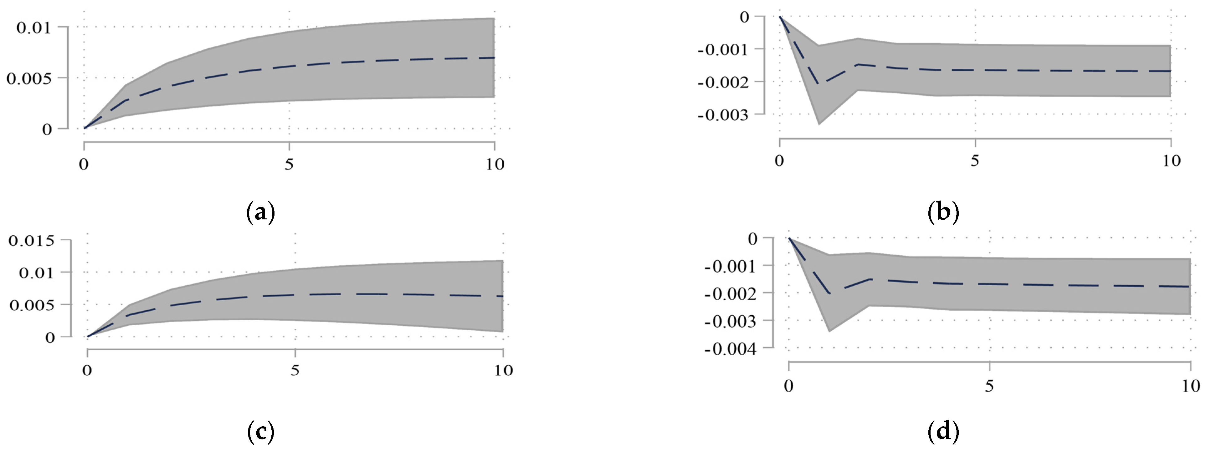
In Figure 5a–d, we analyze the impulse response for household debt and the oil price on economic growth for the parsimonious (P) and comprehensive (C) models with the exogenous variable of the government quality index (GQI). On balance, including the GQI as a control does increase the maximum value of the positive effects of household debt on economic growth, but it does not alter the effects of the oil price on economic growth. This result also suggests that exogenous improvements in the efficiency of social governance arising from government quality upgrades reduce corruption and transaction costs and increase economic efficiency and government quality thereby having a positive effect on household performance.

In Figure 5e–h, we further condition the unrestricted panel VAR with the exogenous effects of financial development. The impulse response shows that including the exogenous variable of financial development as a control weakens the effects of household debt on economic growth. These differences can be explained by the theory that financial development can help improve the efficiency of resource allocation, which lowers the interest rate and risk. Of course, it might persuade consumers to save less and spend more, which likely leads to reduced financial capital accumulation and thereby slows economic growth [40]. Another important finding is that the negative effect of the oil price on economic growth can be alleviated by financial development as an exogenous variable in the parsimonious and comprehensive models. This result also suggests that economic growth is protected by financial development from the impact of oil price shocks.

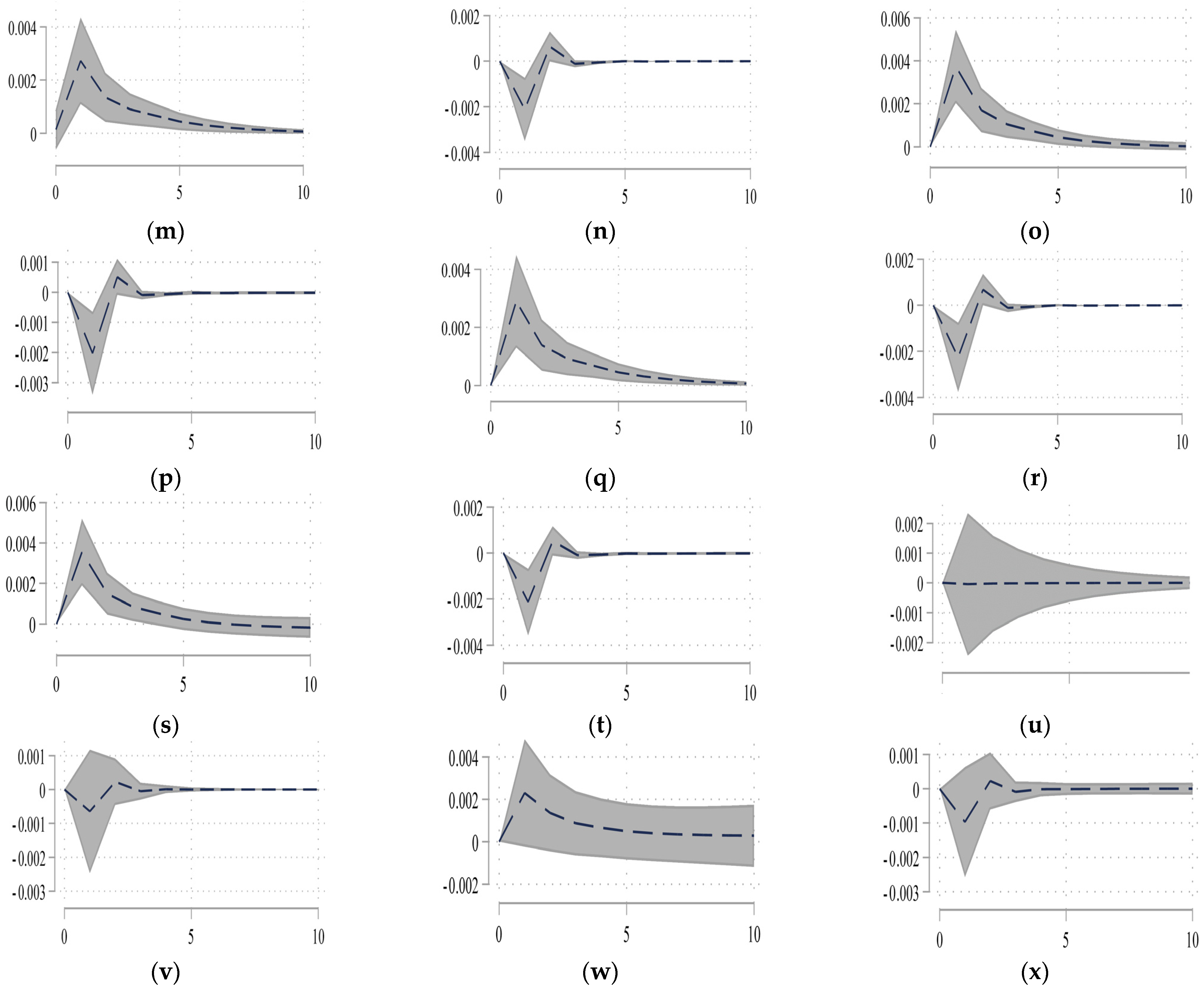
Another set of tests involves increasing the lag count to the higher order VAR (2) systems based on the AIC (Figure 5i–l). The results show that the maximum values of the effects of debt on real output decrease as the number of lags increases and are smoother for the parsimonious and comprehensive models; however, the economic growth response remains positive for a longer time. The impulse response function of the oil price on economic growth leads to a similar conclusion. Next, we alter the order between economic growth and debt for the parsimonious model (Figure 5m,n) or the order between the real exchange rate and the oil price (Figure 5o,p). As the results show in Figure 5m–p, the impulse response functions do not change much. We also control for oil-producing and oil-importing countries. In order to provide a criterion for the division, based on whether this country belonged to OPEC+ countries, 34 countries fell into two groups: OPEC+ countries and non-OPEC+ countries. The empirical test result is shown in Figure 5q–x, and the results show that the approach is valid and robust.

5. Alternative Estimators

We then built panel error correction models (ECMs) of a long-run cointegrating relationship between household debt and economic growth. For consistency with our baseline, the error correction model is:

$$\Delta Y_{it}={\phi }_{it}\Delta Y_{i,t-1}+\Delta X_{i,t-1}^{\text{'}}\beta +{\varphi }_i(Y_{i,t-1}-{\overline{X}}_{it}^{\text{'}}{\theta }_i)+{\alpha }_i+{\epsilon }_{it}$$

(2)

where $Y_{it}$ is economic growth and ${\overline{X}}_{it}$ is the $(1\times (n-1))$ vector of endogenous variables excluding economic growth. The error-correction speed of adjustment parameter ${\varphi }_i$ and the long-run coefficients ${\theta }_i$ are of primary interest. ${\alpha }_i$ is a country fixed effect, $\beta$ and ${\phi }_i$ are the short-run coefficients to be estimated, and ${\epsilon }_{it}$ is an error term. We estimate the pooled mean group (PMG), mean group (MG), and dynamic fixed effect (DFE) estimators for model (2), which we summarize in

Table 3. The results of estimates for the ECM model based on unbalanced panel data.

	$\mathit{\Delta }{\mathit{E}}_{\mathit{i},\mathit{t}}$
	1	2	3	4	5	6
Long-run
$D_{it}$	0.002 ***	0.002 ***	0.003 ***	0.004 ***	0.002	0.003
$R_{it}$		0.000		0.000		0.000
$O_t$	−0.016 ***	−0.017 ***	−0.024 ***	−0.031 ***	−0.019 ***	−0.020 ***
Short-run
$ec$	−1.050 ***	−1.054 ***	−1.017 ***	−1.000 ***	−1.134 ***	−1.154 ***
$\Delta E_{it-1}$	−0.024	−0.033	−0.049	−0.072	−0.012	−0.011
$\Delta D_{it}$	0.001	0.002	0.000	0.001	0.000	0.000
$\Delta R_{it}$		−0.000		−0.001 *		0.000
$\Delta O_t$	0.017 ***	0.020 ***	0.020 ***	0.027 ***	0.022 ***	0.025 ***
Cons	0.006 ***	0.006 ***	0.006 ***	0.005 ***	0.006 ***	0.008
Estimator	PMG	PMG	MG	MG	DFE	DFE
Model	P	C	P	C	P	C
Obs	3500	3199
Ctry	34	34

Note: *, and *** indicate significance at the 10%, and 1% levels, respectively. The PMG estimator constrains the long-run elasticity to be equal across all panels; if the model is heterogeneous, the PMG estimates are inconsistent; the MG estimates are consistent in either case. The Hausman test is used to test the difference in these models. Table 4 shows that the null hypothesis is rejected, and the MG test is efficient.

. One would expect $ec$ (the error correction term) to be negative if the variables exhibit a return to long-run equilibrium; in the results shown in Table 3, $ec$ confirms this expectation. In columns 1–4, the PMG and MG results are estimated: the estimated long-run household debt elasticity is significantly positive, as expected, and the estimated oil price elasticity is significantly negative. Additionally, all estimates reach the 1% significance level.

The DFE estimator, like the PMG estimator, restricts the coefficients of the cointegrating vector to be equal across all panels [41]. The coefficients from the DFE model are similar to the PMG and MG estimates; however, some coefficients are insignificant in the DFE model. In the DFE model, the simultaneous equation bias from the endogeneity between the error term and the lagged dependent variable can be measured by the Hausman test. The result of the Hausman test, in

Table 5. The Hausman test of the DFE and MG estimators.

	MG	DFE	Difference	S.E.	P > chi2
$D_{it}$	0.004	0.003	0.001	0.061	1.00
$O_{it}$	−0.031	−0.020	−0.011	0.336

, shows that the DFE model is preferred over the MG model. Across all these estimators, the research findings show that the oil price has a negative long-term effect and a positive short-term effect on economic growth. The results also show that household debt has a significantly positive long-term effect on economic growth under the PMG and MG estimates.

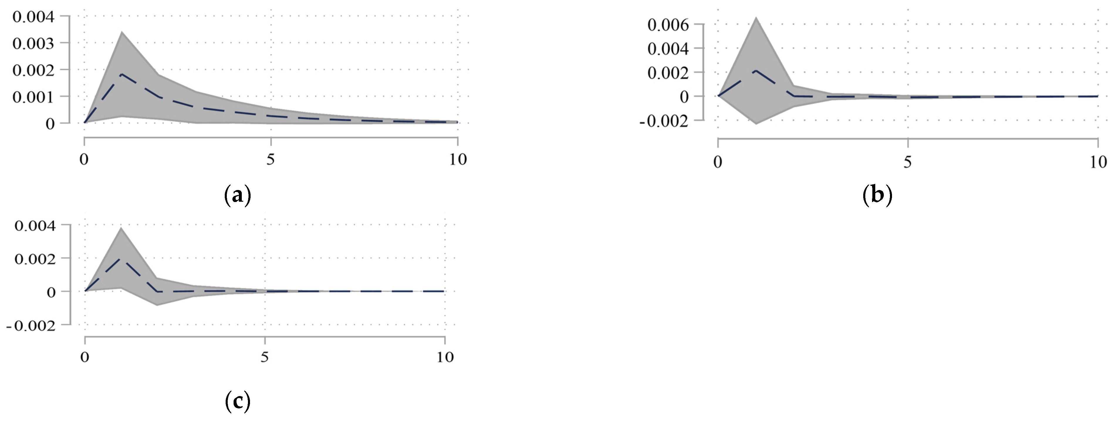
For local projection, this paper discusses the possibility of introducing the pandemic uncertainty index into the model as an exogenous variable. The estimating model is as follows:

$$Y_{it}={\displaystyle \sum _{j=1}^k{Y}_{i,t-j}^{\text{'}}{\mu }_j}+{\alpha }_i+{\epsilon }_{it}$$

(3)

The IRFs of economic growth to household debt and the oil price are shown in Figure 6 and

Table 6. The impulse response estimates for household debt and the oil price on economic growth.

${\mathit{E}}_{\mathit{i}\mathit{t}}$	(1)	(2)	(3)	(4)	(5)
parsimonious
$D_{it}$	0.00246 *	−0.00350 **	−0.000582	−0.00242	−0.000378
$O_t$	−0.0233 ***	0.0124 *	−0.0119	0.0127	0.0231 *
$N$	3124	3090	3056	3022	2988
$R^2$	0.378	0.077	0.022	0.004	0.004
comprehensive
$D_{it}$	0.00263 *	−0.00380 **	−0.000571	−0.00254	−0.000469
$O_t$	−0.0241 ***	0.0123 *	−0.0119	0.0127	0.0229 *
$N$	3112	3090	3056	3022	2988
$R^2$	0.472	0.079	0.022	0.005	0.004

Note: *, **, and *** indicate significance at the 10%, 5%, and 1% levels, respectively. We used the Granger causality test to analyze the inherent relationship between household debt, the oil price and economic growth (Table 7). The results of the Granger causality tests and impulse response functions in the local projection model further prove the baseline conclusion.

, estimated via local projections, for the parsimonious model and comprehensive model. The results show that the positive response of household debt to economic growth and the negative response of the oil price to economic growth are significant for about one quarter, which is consistent with the results from the VAR model. However, in the second quarter, household debt and the oil price also have a significant influence on economic growth, but the influence direction changes, while it is significant only through approximately two quarters.

6. Further Research

There is a tight relationship between bank credit and household debt, in which bank financing is an important component of household debt; it provides capital and credit to families purchasing homes and services, students attending college, and so on. This topic is analyzed and discussed in this paper through empirical analysis (Lim, 2019). We empirically researched and examined the IRFs for a bank debt impulse on household debt. The results are shown in Figure 7. In analyzing the IRFs, we limited our attention to subsamples of developing and developed countries. The results show that the effect of bank debt on household debt lasts 10 quarters. What is remarkable about the IRFs is the degree, direction, and duration of the response; this makes it easy to draw the generalization that bank debt expansion tends to boost household debt and ultimately accelerate economic growth. In this paper, we do not decompose the factors influencing household debt and focus on the short-term effect of the debt as a whole on economic growth. Given a strong positive relationship between the number of children in a family and household debt [42], an additional long-term effect of several components of the debt, such as, for example, financing parental expenditures on the human capital [43] and health [44] of their offspring by resources constrained families could be expected.

7. Conclusions

We contribute to the vast literature on the effects of household debt and oil price on economic growth, and we formulate an unrestricted homogeneous panel VAR model, error correction model, and local projection model. We find that household debt has a positive impact on economic growth; this impact is lagged and gradually decreases, while oil price shocks have a dramatic negative effect on economic growth. In addition, the pandemic uncertainty index has an obvious and positive effect on household debt, while it has an obvious and negative effect on economic growth and oil price. The IRFs and cumulative orthogonal impulse responses for household debt and oil price to economic growth for the parsimonious and comprehensive models tend to decrease over time, especially in an open economy setting. The results from local projections show that household debt alone may only have short-term positive effects on the economy; it should be an addition to stimulus policies, not a substitute for traditional stimulus, such as monetary policy and fiscal policy [36,45]. These conclusions are further confirmed by robustness tests, and these results correspond with the initial hypothesis. This paper’s research results agree with those of literature, such as Liaqat and Ahmed [26] and Wei [30], and show that the methods are robust and stable.

At present, there are many mature papers that focus on public debt; our paper is a first step to understanding the relation between household debt, oil price, and economic growth in the shadow of pandemic. We have considered the simplified model and focused on one key aspect of the pandemic—as exogenous shocks to economic activity. This strategy has allowed us to focus on the interactions between endogenous variables. Although the unrestricted VAR results are very sensitive to misspecification concerns, the validity of these results for a set of perturbations is verified by the results shown in Section 4. Meanwhile, the long-term effects of household debt and the oil price are another important and ongoing area of study. We have made some meaningful advances in this regard, and the results are shown in Table 3.

According to the research conclusion, from a policy perspective, it should be noted that the oil price raising clearly impedes on economy, and especially so for non-OPEC+ countries. In attempts to help promote economic growth, governments need to formulate energy policies that bring energy costs down. The increase of household debt is influenced by a number of factors, government and financial institutions should create services to meet the demand with household debt; the household debt of sustainable development would benefit economic growth. The impacts of the pandemic on household debt, oil price, and economic growth cannot be overlooked [5,6,27]. Notably, several crises occurred during 1965Q1–2021Q3. We agree that the behavior of household debt and oil prices during crises is worth studying. A single topic from different methodological points of view is needed according to which our team want to dig into the problem and take the work a step further for future study.

References

1. Lim, J.J. Growth in the shadow of debt. J. Bank. Financ. 2019, 103, 98–112. [Google Scholar] [CrossRef] [Green Version]
2. Henry, C. Investment decisions under uncertainty: The “irreversibility effect”. Am. Econ. Rev. 1974, 64, 1006–1012. [Google Scholar]
3. Bernanke, B.S. Irreversibility, uncertainty, and cyclical investment. Q. J. Econ. 1983, 98, 85–106. [Google Scholar] [CrossRef] [Green Version]
4. Van Eyden, R.; Difeto, M.; Gupta, R.; Wohar, M.E. Oil price volatility and economic growth: Evidence from advanced economies using more than a century’s data. Appl. Energy 2019, 233, 612–621. [Google Scholar] [CrossRef] [Green Version]
5. Hanspal, T.; Weber, A.; Wohlfart, J. Exposure to the COVID-19 stock market crash and its effect on household expectations. Rev. Econ. Stat. 2021, 103, 994–1010. [Google Scholar] [CrossRef]
6. Waliszewski, K.; Warchlewska, A. Comparative analysis of Poland and selected countries in terms of household financial behaviour during the COVID-19 pandemic. Equilibrium. Q. J. Econ. Econ. Policy 2021, 16, 577–615. [Google Scholar]
7. Krugman, P. Financing vs. forgiving a debt overhang. J. Dev. Econ. 1988, 29, 253–268. [Google Scholar] [CrossRef] [Green Version]
8. Batini, N.; Melina, G.; Villa, S. Fiscal buffers, private debt, and recession: The good, the bad and the ugly. J. Macroecon. 2019, 62, 103044. [Google Scholar] [CrossRef]
9. Liu, K.; Fan, Q. Credit expansion, bank liberalization, and structural change in bank asset accounts. J. Econ. Dyn. Control 2021, 124, 104066. [Google Scholar] [CrossRef]
10. Snieska, V.; Burkšaitienė, D. Panel data analysis of public and private debt and house price influence on GDP in the European Union countries. Inžinerinė Ekon. 2018, 29, 197–204. [Google Scholar] [CrossRef] [Green Version]
11. Caner, M.; Fan, Q.; Grennes, T. Partners in debt: An endogenous non-linear analysis of the effects of public and private debt on growth. Int. Rev. Econ. Financ. 2021, 76, 694–711. [Google Scholar] [CrossRef]
12. Panizza, U.; Presbitero, A.F. Public debt and economic growth: Is there a causal effect? J. Macroecon. 2014, 41, 21–41. [Google Scholar] [CrossRef]
13. Mitze, T.; Matz, F. Public debt and growth in German federal states: What can Europe learn? J. Policy Model. 2015, 37, 208–228. [Google Scholar] [CrossRef]
14. Eberhardt, M.; Presbitero, A.F. Public debt and growth: Heterogeneity and non-linearity. J. Int. Econ. 2015, 97, 45–58. [Google Scholar] [CrossRef]
15. Lof, M.; Malinen, T. Does sovereign debt weaken economic growth? A panel VAR analysis. Econ. Lett. 2014, 122, 403–407. [Google Scholar] [CrossRef] [Green Version]
16. Arcand, J.L.; Berkes, E.; Panizza, U. Too much finance? J. Econ. Growth 2015, 20, 105–148. [Google Scholar] [CrossRef]
17. Schularick, M.; Taylor, A.M. Credit booms gone bust: Monetary policy, leverage cycles, and financial crises, 1870–2008. Am. Econ. Rev. 2012, 102, 1029–1061. [Google Scholar] [CrossRef] [Green Version]
18. Cecchetti, S.G.; Mohanty, M.S.; Zampolli, F. The real effects of debt. SSRN 2011, 352. Available online: https://papers.ssrn.com/sol3/papers.cfm?abstract_id=1946170 (accessed on 20 August 2022).
19. Baum, A.; Checherita-Westphal, C.; Rother, P. Debt and growth: New evidence for the euro area. J. Int. Money Financ. 2013, 32, 809–821. [Google Scholar] [CrossRef] [Green Version]
20. Schmitt-Grohé, S.; Uribe, M. Downward nominal wage rigidity, currency pegs, and involuntary unemployment. J. Political Econ. 2016, 124, 1466–1514. [Google Scholar] [CrossRef] [Green Version]
21. Demirgüç-Kunt, A.; Feyen, E.; Levine, R. The evolving importance of banks and securities markets. World Bank Econ. Rev. 2013, 27, 476–490. [Google Scholar] [CrossRef] [Green Version]
22. Mian, A.; Sufi, A.; Verner, E. Household debt and business cycles worldwide. Q. J. Econ. 2017, 132, 1755–1817. [Google Scholar] [CrossRef] [Green Version]
23. Taylor, A.M. Global financial stability and the lessons of history: A review of Carmen M. Reinhart and Kenneth S. Rogoff’s this time is different: Eight centuries of financial folly. J. Econ. Lit. 2012, 50, 1092–1105. [Google Scholar] [CrossRef]
24. Mian, A.; Sufi, A. House price gains and US household spending from 2002 to 2006. NBER 2014, 20152. Available online: https://www.nber.org/papers/w20152 (accessed on 5 August 2022).
25. Martin, P.; Philippon, T. Inspecting the mechanism: Leverage and the great recession in the Eurozone. Am. Econ. Rev. 2017, 107, 1904–1937. [Google Scholar] [CrossRef] [Green Version]
26. Liaqat, Z.; Ahmed, M.F. Asymmetric effects of private debt on income growth. BE J. Macroecon. 2022, 4. [Google Scholar] [CrossRef]
27. Yu, Y.; Guo, S.; Chang, X. Oil price volatility and economic performance during COVID-19 and financial crises of 2007–2008. Resour. Policy 2022, 75, 102531. [Google Scholar] [CrossRef]
28. Hamilton, J.D. Oil and the macroeconomy since World War II. J. Political Econ. 1983, 91, 228–248. [Google Scholar] [CrossRef]
29. Herrera, A.M.; Karaki, M.B.; Rangaraju, S.K. Oil price shocks and US economic activity. Energy Policy 2019, 129, 89–99. [Google Scholar] [CrossRef]
30. Wei, Y. Oil price shocks, economic policy uncertainty and China’s trade: A quantitative structural analysis. N. Am. J. Econ. Financ. 2019, 48, 20–31. [Google Scholar] [CrossRef]
31. Balashova, S.; Serletis, A. Oil prices shocks and the Russian economy. J. Econ. Asymmetries 2020, 21, e00148. [Google Scholar] [CrossRef]
32. Akinlo, T.; Apanisile, O.T. The impact of volatility of oil price on the economic growth in sub-Saharan Africa. Br. J. Econ. Manag. Trade. 2015, 5, 338–349. [Google Scholar] [CrossRef]
33. Mlaabdal, S.; Chygryn, O.; Kwilinski, A.; Muzychuk, O.; Akimov, O.O. Economic Growth and Oil Industry Development: Assessment of the Interaction of National Economy Indicators. In Proceedings of the 36th International Business Information Management Association (IBIMA). 2021; pp. 8102–8114. Available online: https://ep3.nuwm.edu.ua/22381/ (accessed on 16 October 2022).
34. Abaas, M.S.M.; Chygryn, O.; Kubatko, O.; Pimonenko, T. Social and economic drivers of national economic development: The case of OPEC countries. Probl. Perspect. Manag. 2018, 16, 155–168. [Google Scholar]
35. Akimova, L.M.; Khomiuk, N.L.; Bezena, I.M.; Lytvynchuk, I.L.; Petroye, O. Planning of socioeconomic development of the territories. Int. J. Manag. 2020, 11, 567–575. [Google Scholar]
36. Umaña-Hermosilla, B.; Fuente-Mella, H.; Elórtegui-Gómez, C.; Fonseca-Fuentes, M. Multinomial logistic regression to estimate and predict the perceptions of individuals and companies in the face of the COVID-19 pandemic in the Ñuble region, Chile. Sustainability. 2020, 12, 9553. [Google Scholar] [CrossRef]
37. Kaminskyi, A.; Nehrey, M.; Rizun, N. The impact of COVID-induced shock on the risk-return correspondence of agricultural ETFs. In 2020 Special Edition of International Conference on Monitoring, Modeling and Management of Emergent Economy. M3E2-MLPEED; 2020; pp. 204–218. Available online: https://pesquisa.bvsalud.org/global-literature-on-novel-coronavirus-2019-ncov/?lang=pt (accessed on 16 October 2022).
38. Levine, R. Finance and growth: Theory and evidence. Handb. Econ. Growth 2005, 1, 865–934. [Google Scholar]
39. Greiner, A. Economic growth, public debt and welfare: Comparing three budgetary rules. Ger. Econ. Rev. 2011, 12, 205–222. [Google Scholar] [CrossRef]
40. Blanchard, O.J. Debt, deficits, and finite horizons. J. Political Econ. 1985, 93, 223–247. [Google Scholar] [CrossRef] [Green Version]
41. Blackburne, E.F., III; Frank, M.W. Estimation of nonstationary heterogeneous panels. Stata J. 2007, 7, 197–208. [Google Scholar] [CrossRef]
42. Deng, X.; Yu, M. Does the marginal child increase the household debt?—Evidence from the new fertility policy in China. Int. Rev. Financ. Anal. 2021, 77, 101870. [Google Scholar] [CrossRef]
43. Azarnert, L.V. Free education, fertility and human capital accumulation. J. Popul. Econ. 2010, 23, 449–468. [Google Scholar] [CrossRef]
44. Azarnert, L.V. Health capital provision and human capital accumulation. Oxf. Econ. Pap. 2020, 72, 633–650. [Google Scholar] [CrossRef]
45. Lepetit, A.; Fuentes-Albero, C. The limited power of monetary policy in a pandemic. Eur. Econ. Rev. 2022, 104168. [Google Scholar] [CrossRef]
Figure 1. Household debt as a share of GDP and the crude oil price.
Sustainability 14 15140 g001
Figure 2. The impulse responses for household debt and the oil price on economic growth (ad) and economic growth on household debt and the oil price (eh) for 10 quarters after the shock. The dark gray areas indicate the 95% confidence intervals generated using Gaussian approximation of 200 Monte Carlo draws from a fitted unrestricted panel VAR model. (a) Household debt on economic growth (P). (b) Oil price on economic growth (P). (c) Household debt on economic growth (C). (d) Oil price on economic growth (C). (e) Economic growth on household debt (P). (f) Economic growth on oil price (P). (g) Economic growth on household debt (C). (h) Economic growth on oil price (C).
Sustainability 14 15140 g002
Figure 3. Cumulative orthogonal impulse responses for household debt and the oil price on economic growth for the parsimonious and comprehensive models. (a) Debt on growth, parsimonious. (b) Oil price on growth, parsimonious. (c) Debt on growth, comprehensive. (d) Oil price on growth, comprehensive.
Sustainability 14 15140 g003
Figure 4. The impulse response of different types of debt on economic growth. (a) Bank credit on economic growth. (b) Government debt on economic growth. (c) Private debt on economic growth.
Sustainability 14 15140 g004
Figure 5. The impulse responses of economic growth based on different models. (a) Household debt (GQI, P). (b) Oil price (GQI, P). (c) Household debt (GQI, C). (d) Oil price (GQI, C). (e) Household debt (Financial, P). (f) Oil price (Financial, P). (g) Household debt (Financial, C). (h) Oil price (Financial, C). (i) Household debt (VAR(2), P). (j) Oil price (VAR(2), P). (k) Household debt (VAR(2), C). (l) Oil Price (VAR(2), C). (m) Household debt (Alter order, P). (n) Oil price (Alter order, P). (o) Household price (Between order, C). (p) Oil price (Between order, C). (q) Household debt (Non-OPEC+, P). (r) Oil price (Non-OPEC+, P). (s) Household debt (Non-OPEC+, c). (t) Oil price (Non-OPEC+, C). (u) Household debt (OPEC+, P). (v) Oil price (OPEC+, P). (w) Household debt (OPEC+, C). (x) Oil price(OPEC+, C).
Sustainability 14 15140 g005aSustainability 14 15140 g005b
Figure 6. The IRFs of economic growth to household debt and the oil price. (a) Household debt on economic growth (P). (b) Oil price on economic growth (P). (c) Household debt on economic growth (C). (d) Oil price on economic growth (C).
Sustainability 14 15140 g006aSustainability 14 15140 g006b
Figure 7. The IRFs for a bank credit impulse on household debt. (a) Developed countries. (b) Developing countries. (c) Whole sample.
Sustainability 14 15140 g007