Article

Numerical Simulation of the Thermal Environment during Summer in Coastal Open Space and Research on Evaluating the Cooling Effect: A Case Study of May Fourth Square, Qingdao

1
Department of Landscape Architecture, Central South University of Forestry and Technology, Changsha 410004, China
2
Hunan Big Data Engineering Technology Research Center of Natural Protected Areas Landscape Resources, Changsha 410004, China
3
College of Landscape Architecture and Forestry, Qingdao Agricultural University, Qingdao 266109, China
4
Scientific and Technological Commission, China Urban Construction Design & Research Institute Co., Ltd., Beijing 100120, China
5
College of Civil Engineering and Architecture, Qingdao Agricultural University, Qingdao 266109, China
*
Author to whom correspondence should be addressed.
Sustainability 2022, 14(22), 15126; https://doi.org/10.3390/su142215126
Submission received: 14 October 2022 / Revised: 10 November 2022 / Accepted: 11 November 2022 / Published: 15 November 2022
(This article belongs to the Topic Built Environment and Human Comfort)

Abstract

:
Urban green space is considered an important part of urban ecological construction be-cause of the efficiency of green space in reducing ambient temperature. It was previously reported that the quantity and layout of arbors and paving are very important factors for cooling. To research the combination mode of the quantity and layout of arbors and paving able to effectively lower the temperature during the summer in a coastal open space environment where little architecture exists, we built a numerical model of heat transfer using ENVI–met numerical modeling simulation, for which the May Fourth Square in Qingdao was selected. The results showed that the ratio coverage of the arbor layer and pavement fragmentation were positively correlated with the cooling effect. We found that setting the passageway conformed to the sea breeze by arbors and close planting at the air outlet effectively reduced the site temperature. After optimizing the site’s greening layout, the cooling effect over the process of time decreased in the height direction. At the same time, the cooling effect increased before 15:00 and then reduced gradually in the time dimension. Compared to the original site, the total cooling efficiency reached 1.41 × 10⁸ J, equaling electric energy of about 39.2 kW·h. This research solves the issue of the synergy between planting and pavement for cooling coastal open spaces in summer and provides a basis to formulate a promotion strategy for landscape design areas with similar geographical and climatic conditions.

1. Introduction

The urban heat island (UHI) effect is a local high temperature phenomenon in urban areas [1]. The urban heat island effect continues to rise with an increase in construction intensity heat rejection and at the same time green space and water areas [2]. This is currently an urgent need to alleviate the heat island effect for current urban construction. Additionally, certain climatic conditions are prerequisites for the thermal comfort of the site [3,4]. Research on cooling measures for urban sites under different geographical conditions will be very helpful to mitigate the urban heat island effect.
There have been a lot of studies on how to alleviate the UHI effect. Expanding urban green space coverage has significant effects [5]. The cooling effect of green space varies according to the size and type of green space, the structural characteristics of plants, and the spatial model of green space [6,7,8]. The shape of the green space also impacts the cooling effect. An Israeli study showed that the shape index of green spaces had little impact on cooling effects, but many other studies have shown that shape index plays an important role in cooling effects [9,10,11,12]. Some scholars have noted that certain methods are beneficial to alleviate the UHI effect and increase thermal comfort including reducing man-made heat and pavement area and aggregation, and increasing plant coverage [13]. In addition to plants, water can also significantly alleviate the heat island effect. By using the method of land surface temperature inversion, it was found that the heat island intensity is obviously reduced in the waters of the Nanjing section of the Yangtze River, Shijiu Lake, and Gucheng Lake [14].
At present, the quantitative research methods of urban thermal environment include ground observation, remote sensing, and numerical simulation [15]. Numerical simulation can be used for three-dimensional simulation of thermal environment, and computational fluid dynamics (CFD) is one of the most commonly used numerical simulation methods. CFD includes ANSYS Fluent, PHOENICS, ENVI-Met, CFX, Star-CD, and Star-CCM. With CFD technology, the convection, heat conduction, and radiant heat transfer in the urban space can be coupled to predict the urban thermal environment [16]. At present, many studies have proposed methods and measures to improve urban thermal environment based on CFD technology, including rational layout and optimization of plants, water, buildings, and urban ventilation corridors. However, these studies lack quantitative research on landscape elements and usually focus on a single landscape element, lacking systematic research on the effects of multiple elements on thermal comfort.
Based on the research status, this study focuses on how to make the wind, pavement, and plants work together to produce a cooling effect in the urban open space next to large water (the ocean) so as to obtain a better thermal environment. Therefore, hot summer climate conditions, field investigation, and the ENVI–met simulation method were selected for the study. The results of this study could help mitigate the urban heat island effect by providing a reasonable green space layout mode and improving cooling efficiency.

2. Materials and Methods
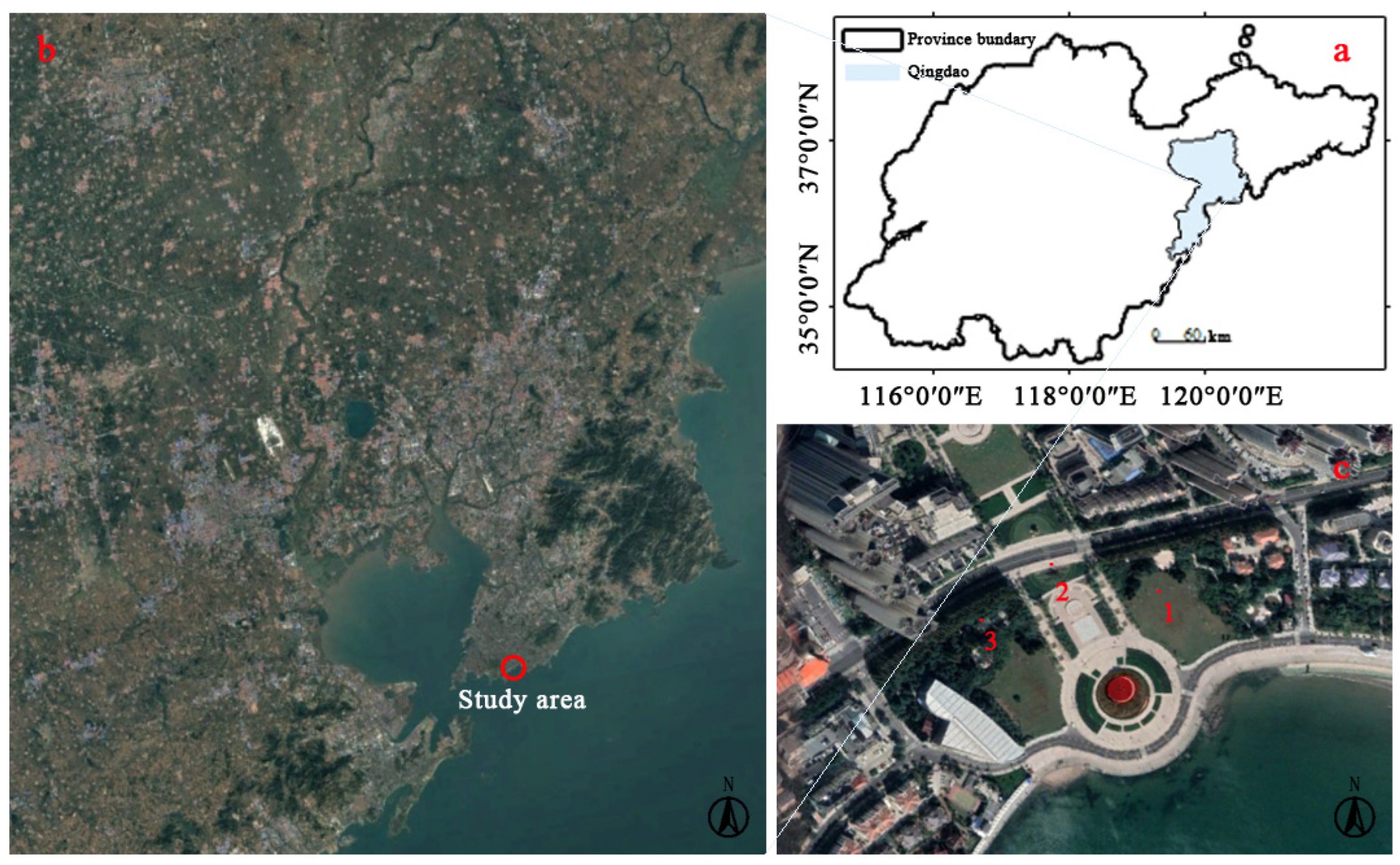
2.1. Research Area

Qingdao is located between 119°30′–121°0′ E and 35°35′–37°9′ N and is geographically situated in the east coast of China. The average maximum temperature in the area is mostly between 24.0 and 30.0 °C in the summer. The southeast wind prevails there, with average wind speeds between 3.4 and 5.4 m/s in the summer [17]. The summer monsoon can bring cool and humid air over the ocean into the city. The May Fourth Square site, which covers an area of 8.5 hectares, faces the Yellow Sea to the south at the edge of the city. This site serves as an urban public green space. The geographical location of Qingdao is shown in Figure 1a. The location of the study area in Qingdao is shown in Figure 1b. Points 1–3 in Figure 1c are the actual measurement points arranged according to lawn, pavement, and dense forest. The pavement concentrated in the central layout of the site accounts for 35% of the total. The buildings scattered in the green space account for 1.5%. Arbors concentrated in the north account for 28%. There is no shade in the main crowd activity area, and little space exists for activities under the forest of the site. The area does not meet the requirements of human thermal comfort in the summer.

2.2. Methodology

2.2.1. Technical Route
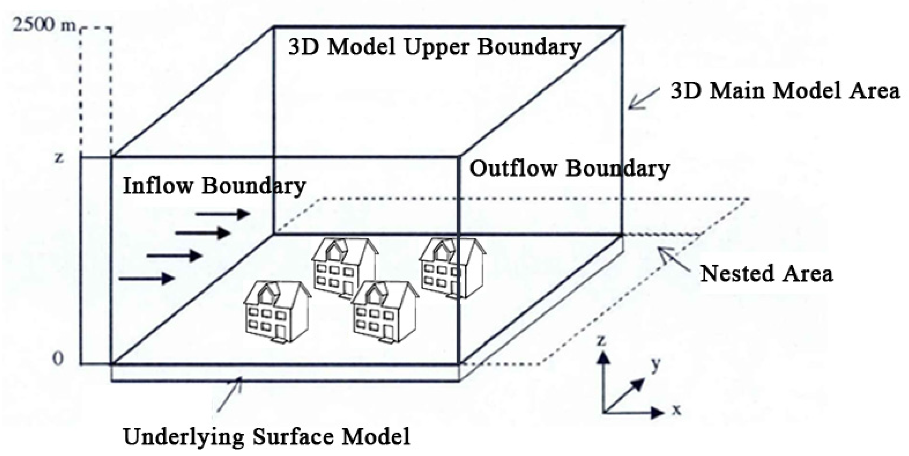
In this study, we conducted field research to obtain the physical environment parameters and typical sunny-day climate data during the summer at the May Fourth Square. These data were then used as the initial condition and initial climate parameters for ENVI–met software modeling. We first created the site status model as the control group and then established multiple models according to different underlying surfaces and planting layout modes. Software simulations output microclimate data to analyze in comparison with the current situation. In this way, we sought to obtain the best design pattern to satisfy the summer cooling needs of the site and analyze the ultimate cooling efficiency of the designed site.
ENVI–met can simulate surface–plant–air interactions in urban environments based on the principles of fluid mechanics, thermodynamics, and atmospheric physics [18]. Some scholars previously evaluated the accuracy of models showing that the urban cooling effect would change according to the urban form, the type and scope of vegetation, and the time period of heat mitigation [19]. The model is composed of a 3D master model, one-dimensional boundary model, and nested grids (Figure 2).
Thermal effect studies based on ENVI–met typically follow a three-step study workflow, which is universal in numerical simulation research. These steps are modeling, verification, and scene simulation. We also used these three steps to simulate and analyze the climatic environment of the coastal open space.

2.2.2. Model Setup

ENVI–met V5.0.2 was used for simulations in this study. The simulation site was set to be 500 m long and 500 m wide and used multiple nested grids. We set the number of model grids to 125 × 125 × 30 to represent the space of the whole site. Meteorological data of typical sunny days in July in Qingdao city were used as the initial value to simulate the thermal environment under different scenarios (Table 1) (Source: combination of data published by local meteorological department, national meteorological data center, and measured data).
The underlying surface and planting layouts are the most important factors that determine the physical environment of the site without changing the existing buildings. In terms of the underlying surface, primarily loamy soil and granite pavement set to default values were used during the simulation. For planting, the software provided plant modeling parameters set according to plant physiological characteristics. Black pine was chosen as a representative plant because it is the most widely used species in seaside areas in Qingdao city. We used the canopy meter (LAI-2200) to determine the leaf area index LAI of dominant species. The LAD values of plants with the given tree height, crown width, and under branch height were calculated using Formula (1):
L A I = 0 h L A D · Δ z
where L A I = the leaf area index, L A D = the leaf area density, Δ z = the crown height of each layer, and h = the crown height [20].
The plant model parameters, according to the relevant measurements and calculations, are shown in Table 2.

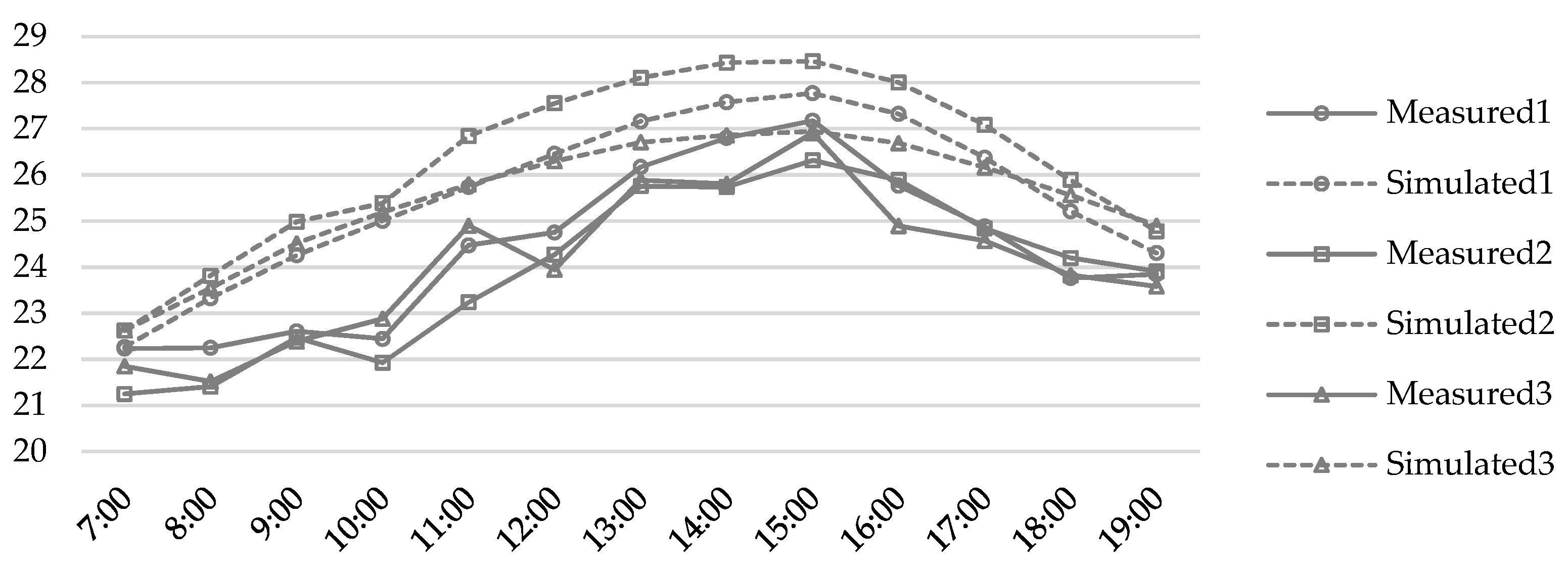
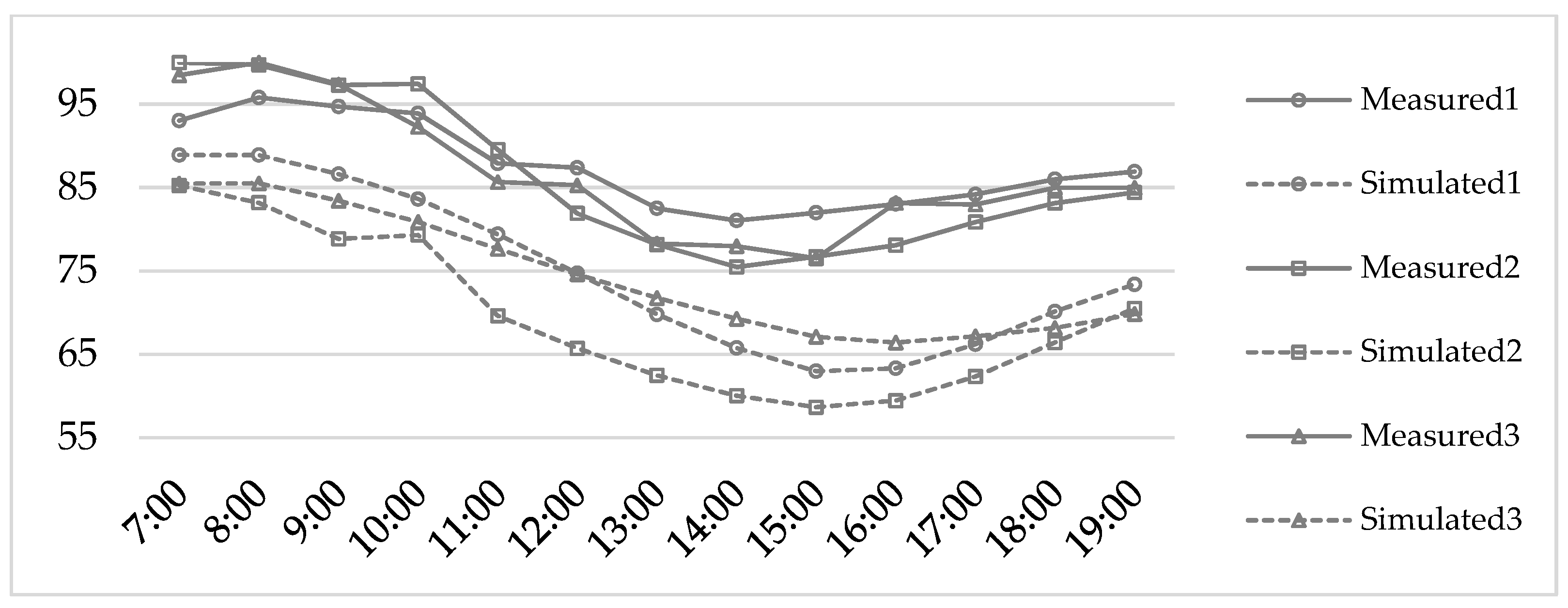
2.2.3. Model Validation

It is necessary to conduct in situ measurement verifications for research and analysis with ENVI–met. Data on air temperature, relative humidity, and wind speed have been used for actual measurement verification in several studies [18]. The typical sunny day climate parameters of Qingdao in summer were selected as the initial values for simulation (Table 1). The software vendor considers the minimum simulation time required to study UHI to be 24 h. Thus, the simulation duration was set to 24 h. We conducted measurements on 15 July 2022, which was a sunny day with typical summer climate characteristics in Qingdao. The measured time was set from 7:00 to 18:00. Three points were measured (Figure 1). We measured the data at ten-minute intervals of 30 s before and after each hour at 1.4 m, which is considered pedestrian height. The average values were taken as the measured hourly climate data (Table M01 of Supplementary Materials). Next, the measured values and simulated values were statistically analyzed. The root mean square error (RMSE), systematic RMSE (RMSEs), unsystematic RMSE (RMSEu), and index of agreement (d) were chosen to evaluate the accuracy of the temperature and humidity of the model. The RMSEs explain the part of the total error that always occurs and has specific causes, such as the errors caused by weak characterization of the research object due to using the meshing method in the ENVI–met model. RMSEu is composed of input parameters, the accuracy of the constructed model, empirical constants, etc. The index of agreement (d) is the probability that the simulated value of the model agrees with the measured value. This value indicates how accurately the model predicts a variable, where D = 1 means that the simulated value is completely consistent with the measured value. The expression formula is as follows:
d = 1 i = 1 n ( P i O i ) 2 i = 1 n ( P i O i ) 2 ,   0 d 1
R M S E s = 1 n i = 1 n ( P i ^ O i ) 2
R M S E u = 1 n i = 1 n ( P i P i ^ ) 2  
R M S E = R M S E u 2 + R M S E s 2
where n = measured times, P i = simulated value, O i = measured value, P i = simulated average value, O i = measured average value, and P i ^ = vector of the simulated value.
The temperature simulation error of the three measuring points is between 0.04 and 3.6 °C, in which the error of measuring point 1 is the smallest and that of measuring point 2 is larger. The simulation error of humidity is between 4% and 20%, the error of measuring points 1 and 3 is small, and that of measuring point 2 is large. The error is within the acceptable range. We quantitatively evaluated the error between the simulated and observed values of atmospheric temperature and relative humidity (Table 3), finding that the R2 values of all measuring points were greater than 0.78, and the RMSEs were greater than the RMSEu. This result might be due to the low air humidity in the ENVI–met initial parameter settings. The temperature RMSE value was found to be between 1.4 and 2.6 °C. The humidity RMSE was recorded as 12.8–17.5%. The errors were within an acceptable range. This result shows that the variation trend of the simulated value is consistent with that of the measured value, which means that the simulation can accurately predict changes in site temperature and humidity (Table M02 of Supplementary Materials).
The corresponding diagrams show that the temperature error is small between the simulated value and the observed value of the three measuring points (Figure 3), which have the same trend of changes in the three points. Overall, the simulated temperature is higher than the observed value, and the simulated humidity value is lower than the observed value (Figure 4). This result may be due to the high humidity of the seaside air on the day of observation. The thermal radiation of the square pavement was greatly reduced as humidity reached close to 100% for many hours in the morning. Due to this humidity, the observed near-surface temperature was lower than the simulated value.
In terms of wind speed, static inputs are used to represent wind speed and direction in the ENVI–met model. The validation study shows that models have trouble predicting the dynamic behavior within a day [21].
Although the simulation effect of dynamic changes in wind speed data is poor, the wind speed value mainly depends on the physical environmental conditions and climatic conditions. Therefore, the changes in wind speed and direction generated by the software simulation reflect the relationship between the site status and the climate environment. The simulation data for wind speed are, therefore, of reference value.

2.2.4. Construction of Simulation Models

The long-wave radiation of the pavement has a heating effect on the air. The area ratio of the underlying surface and the patch area are the key pattern features that affect the temperature and humidity of the micro-scale environment. The degrees of fragmentation and aggregation also have some influence [22]. Considering that the current pavement of the site is too concentrated, we applied two pavement layout methods to make the pavement layout more decentralized. Secondly, based on the cooling and humidifying effects of plants, we set different planting positions and types of tree coverage to explore the cooling effect of the planting layout mode. The specific settings are outlined in Table 4 (Models C01–C07 of Supplementary Materials).
To keep the climate condition parameter settings consistent, case 1 (the current situation) was compared with other models with different underlying surfaces and planting layouts as the control group. Control cases 2 and 3 were designed to analyze the cooling effects of different underlying surfaces. Cases 2 and 3 have the same greening and pavement coverage as model 1 but with different pavement fragmentation levels. This setting reflects the cooling effects of different pavement layout modes. Control case 4 aims to analyze the cooling effects of different planting positions. Case 4 has the same pavement layout and arbor coverage as case 1 and reflects the influence of planting position on site temperature by planting arbors with 28% coverage on the south side of the site where the wind comes from. Arbor coverage reaches 37% in Scenario 5. The east and west sides of the site are planted in a row along the dominant wind direction to form an air duct. Here, the planting width and row spacing are set to 10 m to effectively form a wind channel [23].
The purpose of comparing cases 6 and 7 is to analyze the cooling effect of increasing tree coverage and forming air ducts. Case 6 increases the arbor coverage to 50%, where dense plant coverage in the north of the site and plants in the south of the site form an air duct. Case 7 sets the arbor coverage rate to 50% but with dense plants on the south side of the site and an air passage on the north side. Comparative analysis of the simulation results for model 6 and 7 shows the cooling effect under different positional relationships between the planting layout and sea breeze direction. Finally, according to the simulation analysis results of the 7 cases, we obtained an optimal solution for the landscape construction mode of coastal open space based on summer cooling demand. Furthermore, the overall cooling effect in three-dimensional space was obtained by comparing the optimal model with the current situation.

2.2.5. Evaluation Index

In this section, we quantitatively analyze the impacts of different landscape construction modes on the human thermal comfort index in summer coastal open space and examine the cooling effects of the optimized design mode on the site.
According to frequency of use, the human thermal comfort index includes physiological equivalent temperature (PET), predicted mean vote (PMV), universal thermal climate index (UTCI), comfort formula (COMFA), and temperature of equivalent perception (TEP) [24]. These indices can be calculated from the ENVI–met meteorological output values and can also be directly extracted from BIO-met. PET is the air temperature at which human skin temperature and body temperature reach a thermal state equivalent to that of a typical indoor environment when located in an indoor or outdoor environment [25]. PET is widely used when assessing the micro thermal environment. PET adopts radiant flux from body heat balance in all possible directions and wavelengths, including short wave and long-wave radiation. The human sex, height, age, weight, heat resistance of clothes, and metabolic heat are included in the calculation. Therefore, PET has become the most widely used index in urban climatology and is considered the most suitable for evaluating outdoor human thermal comfort [26]. PET is a thermal comfort index derived from the Munich energy balance model for individuals (MEMI). The MEMI formula is [27]:
M + W + R + C + E D + E R e + E S w + S = 0
where M = metabolic rate, W = work item, R = radiant heat exchange term, C = convective heat flux, and ED = heat loss caused by water evaporation to the surrounding air through the surface when the skin is dry, ERe = sweat heat loss, and ESw = thermal storage.
In this study, the physiological equivalent temperature (PET) output by the BIO-met module in ENVI–met is taken as the thermal comfort index. To perform PET calculation and analysis, the parameter settings are as follows: height = 1.75 m; weight = 75 kg; Age = 35; gender = male; body surface area = 1.91 m2; static clothing insulation index = 0.3; metabolic rate (walking or simple activities) = 86 W·m2.
Three-dimensional cooling effect can be produced by green space formed by planting. Therefore, it is necessary to calculate the three-dimensional space cooling effect including the cumulative effects of temperature reduction and the cooling efficiency of the site [28]. At present, there is no literature on the calculation height of cooling efficiency. The statistical height h is set to 7 m. Simulated temperatures at 0.2, 0.6, 1.0, 1.4, 1.8, 3.0, 5.0, and 7.0 m heights are used for the statistical temperature calculations. The statistical duration is subject to the measured time interval of 7:00–19:00, and the cooling effect is calculated as follows:
Δ T = 0 h [ Ty Td ( h ) ] dh
Δ   Q = cm Δ   T = c ρ s 0 h [ Ty Td ( h ) ] dh
In Formula (7), ∆T is the cumulative value of the temperature difference between the design site temperature and the original site temperature at a height of 0–7 m. Ty is the original site temperature. Td is the temperature of the design site. T(h) is the function of the change of the daily average temperature of the design site relative to the original site with height. The upper integral limit h is the set temperature statistical section height of 7 m. In Formula (8), ∆Q is the cumulative value of the cooling efficiency of the design site within the range of 0–7 m. c(1 × 10³ J/kg·°C) is the specific heat of the air. ρ(1.29 kg/m3) is the air density. s is the total area excluding buildings in the study area.

3. Results

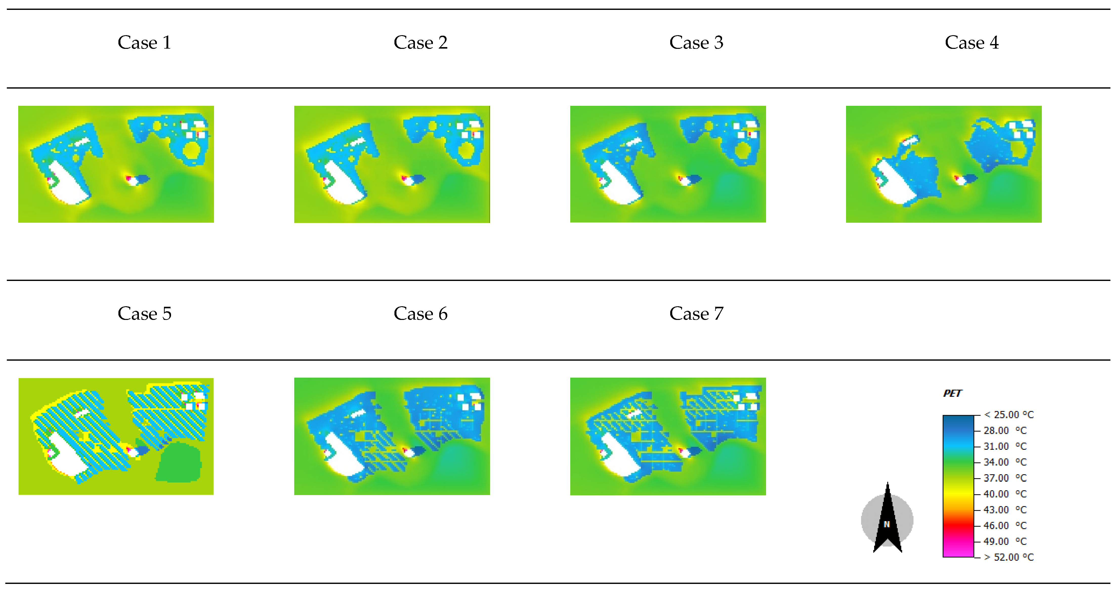
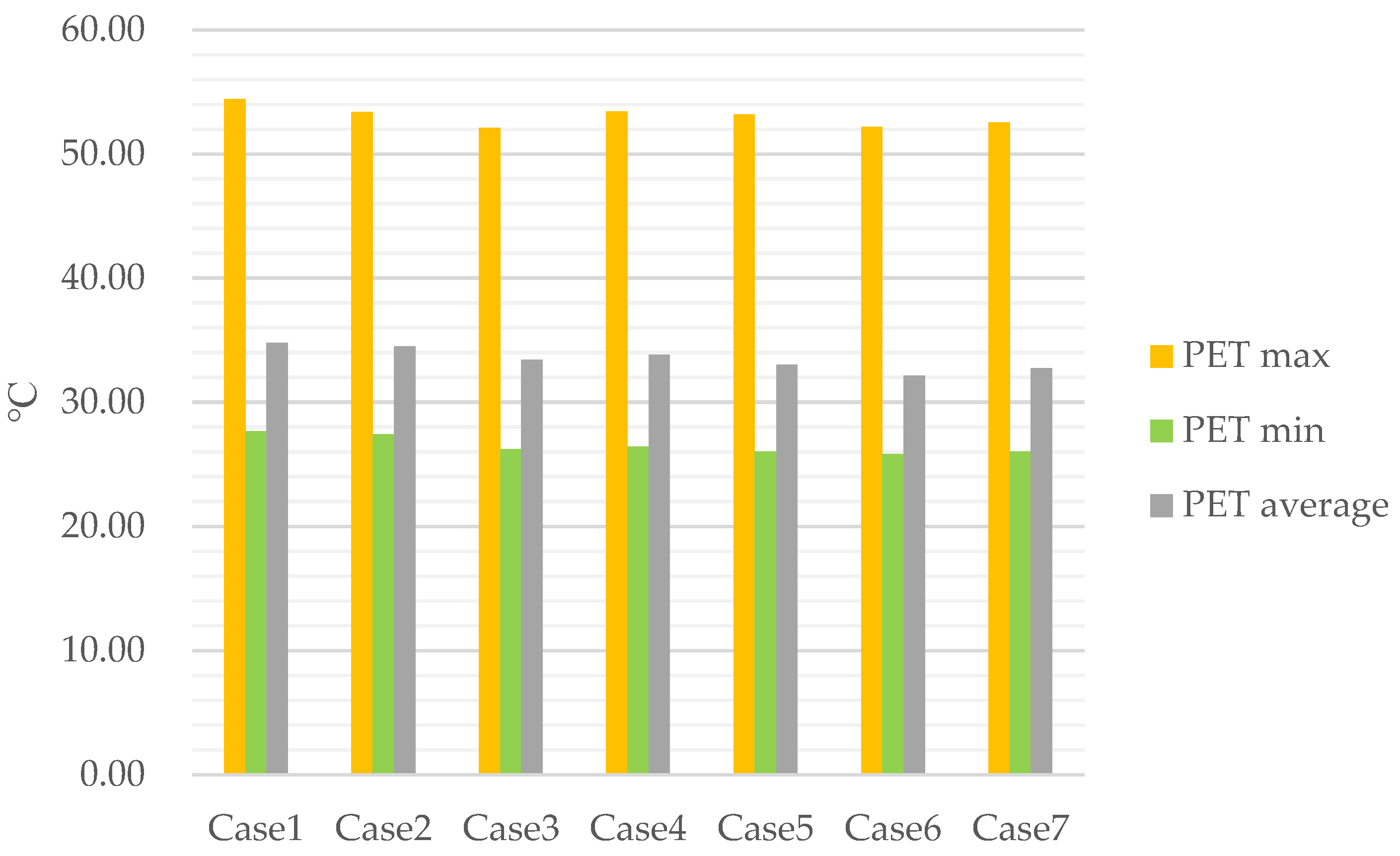
3.1. Analysis of Thermal Comfort

Figure 5 shows the PET distribution planes of six models with a human height of 1.4 m at 15:00. It can be seen that the PET range is between 27.7 and 54.4 °C and that the average PET reaches 34.8 °C under the current conditions in case 1. The cool area is located in the green space under the shadow of the east side of buildings and trees where solar radiation does not directly reach the ground. For this reason, the average radiation temperature in the area is low. Hot spots up to 54.4 °C appear in the quiet wind zone on the northwest leeward side of the building, which is also a position directly exposed to solar radiation. In general, higher PET values were recorded in the paved area under direct sunlight, while lower PET values were observed in shaded areas under forest cover or buildings. At the same time, good ventilation conditions are conducive to reducing PET. Therefore, when designing cases 2–7, we broke the pavement to reduce the heat generated by long-wave radiation and improved planting coverage to form good ventilation conditions, thereby reducing PET (Tables P01–P07 of Supplementary Materials).
The simulation results of cases 2–7 show the thermal comfort of the study area under different pavement and planting layouts. The average PET of all cases is between 32.1 and 34.5 °C (Figure 6), which is lower than the current PET. At the same time, the maximum temperature of all cases is slightly lower than that of case 1, but the location is basically the same as that of case 1, with all maximum temperatures located in the direct sunlight areas with low wind speeds on the northwest sides of the buildings. However, in different cases, the underlying surfaces at these locations are planted and paved, and their long-wave radiation heating effects are different. Therefore, at these locations where extreme high temperatures occur, the west facade of the building receives solar radiation and continuously generates long-wave radiation to the surrounding area, which is the biggest reason for the formation of extreme high temperature at the site.
First of all, the simulation data for cases 1–3 show that under the same pavement coverage, a relatively dispersed pavement layout can effectively reduce PET. The PET of case 1 is between 27.7 and 54.4 °C. Under the same planting conditions, the highest PET and average PET in the whole region of case 2 were reduced by 1.9% and 0.8%, respectively, compared to the current situation. The highest PET and average PET in case 3 (with the highest pavement fragmentation) were 4.2% and 4.0% lower than the status quo because the scattered pavements gain more shade, thus reducing their heat storage and reradiation capacity. The PET values in the three cases all show that the area ratio is close to 50% in the temperature range of 34–37 °C (Figure 7). This condition results in a higher site-average PET. However, compared to cases 1 and 2, the overall temperature of the original central paving area dropped significantly in case 3, and the area with PET values of 28–31 °C accounted for 30.2%, which is much higher than the proportion in cases 1 and 2 due to the cool sea breeze from the southeast passing through the tree-free area first. When the pavement is more dispersed, the long-wave radiation generated by the pavement heats the air less. Cool air is then blocked by the dense forest in the northern part of the site to form a more effective cooling area.
Secondly, the simulation data for cases 1 and 4 show that under the same pavement layout (current situation), the same tree coverage can be concentrated on the south side of the site to achieve a better cooling effect. The maximum PET and average PET of the site are reduced by 1.8% and 2.9%, respectively, compared to the current situation through the concentrated planting of arbors on the south side of the site. The low-temperature area (<31 °C) of the site increased more than the current situation, with these areas concentrated in the southeast side of the site. This occurs because the cool air introduced by the wind from the southeast sea surface is detained on the southeast side of the site due to vegetation blockages, thereby reducing the thermal radiation effect of this part of the centralized pavement. At the same time, this part of the cool air can achieve effective plant cooling when it reaches the area where the plants are concentrated, which makes the area experience a better cooling effect than the current situation, whether it is paved or planted.
Finally, the data for cases 5–7 show that when the fragmentation of pavement is increased, the coverage rate of arbor increases to 50%. At the same time, the wind channel along the dominant summer wind direction is established by planting, and a better cooling effect in summer is obtained. Case 5 uses planting to form a full-field ground wind channel, which decreased the highest and average PET by 3.8% and 7%. Case 6 features densely planted trees on the north side of the site, while the wind channel area formed by trees is set up in the monsoon direction of the site on the southeast side. As a result, the highest and average PET decreased by 4% and 7.8%, respectively. Case 7 features densely planted trees on the south side of the site, with the wind channel area set up on the northwest side of the site. This configuration decreased the highest and average PET by 3.8% and 7%, respectively. It can be seen that the cooling effect of dense arbor planting in the north is better than that in the south. This result seems to contradict the conclusion presented in the previous case 4 but highlights the importance of ventilation for cooling. Densely planted forest land will retain cool air on the southeast sea surface in the south. Additionally, establishing a wind channel at the sea breeze inlet is conducive to cool air entering the site, enabling one to obtain a better overall cooling effect. At the same time, it has been confirmed that there is a significant negative correlation between UHI and aerosol optical depth (AOD) [29]. Attenuation of incident solar radiation caused by high AOD is the cause of low temperature [30]. The range of PET in case 6 below 31 °C reached 53.3% that of the study site area, which is significantly superior to the other cases in terms of the PET mean value, high temperature extreme value, and cool area. Therefore, under the common climate conditions of the Qingdao coastal open space in the summer, the site pavement should be designed in a decentralized manner, and a wind channel should be set up on the windward side to introduce cool sea breeze into the site. At the same time, planting dense forests near the wind direction exit of the site will decrease the temperature of air in the site, thereby achieving a good cooling effect.

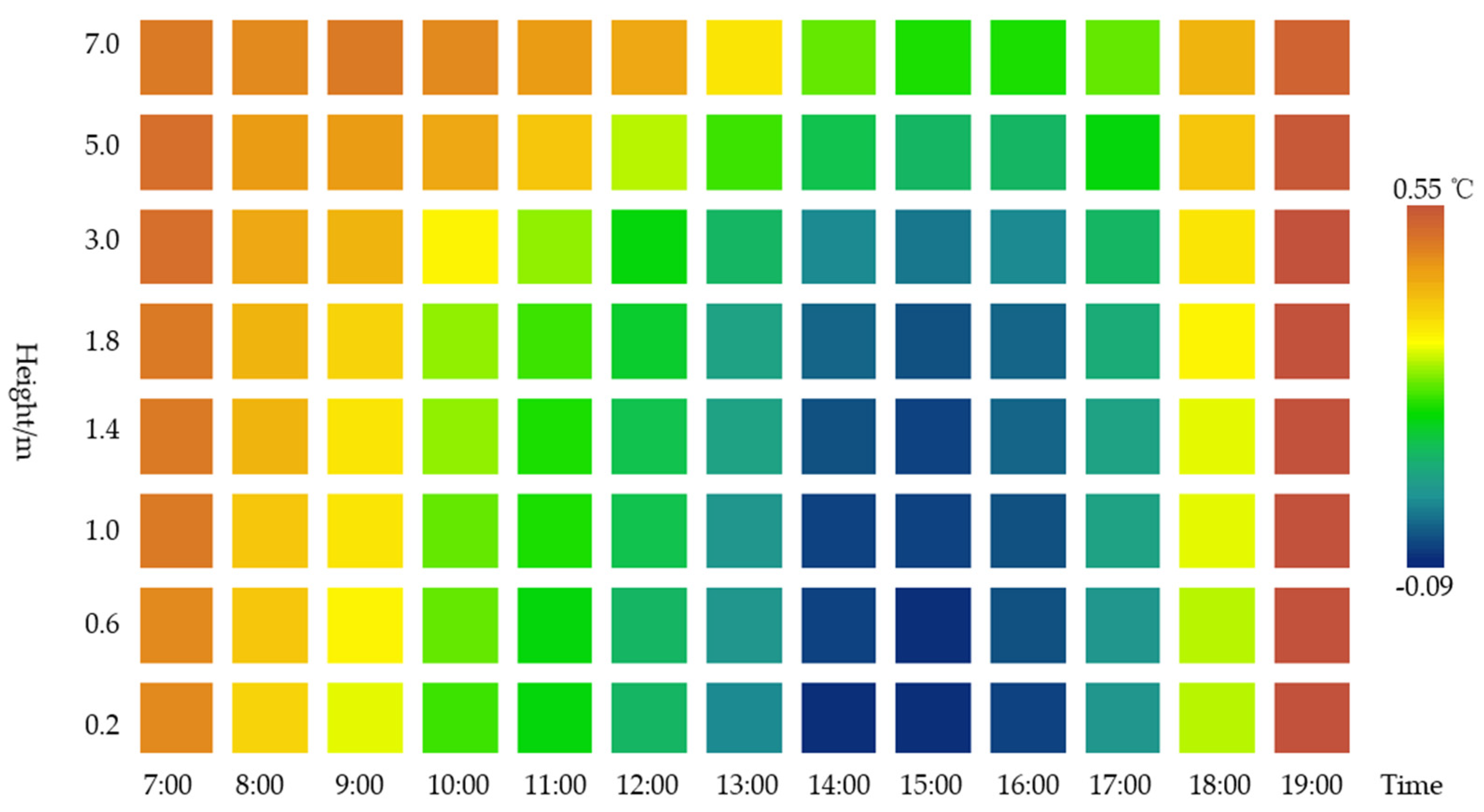
3.2. Analysis of Cooling Efficiency

The following section analyzes the cooling effectiveness of the optimal cooling design case obtained from the previous research and analysis. The average temperature differences of case 6 and case 1 generated in the ENVI–met software for each calculation section height layer were exported to excel, and a table with time point and height as the abscissa and ordinate, respectively, was created (Tables S01–S13 of Supplementary Materials). Each datum in the table represents the mean temperature difference at a certain height at a time node. To visualize the data, each datum in this table was assigned corresponding x and y coordinate values in the order of natural numbers. Then, the data were imported into the GIS software and colored according to the average temperature difference data. The resulting distribution diagram of the average temperature differences (with height and time) between case 6 and case 1 in the study area is shown in Figure 8.
According to the simulation data and the average temperature drop statistics of case 6 compared to case 1 at each time node and height in the study area (Figure 9, Figure 10 and Figure 11), the average temperature drop range is −0.09–0.55 °C, and the minimum average temperature drop occurs at 19:00 at a 3 m height. The maximum average temperature drop occurs at 15:00 at a height of 0.2 m. The overall cooling feature is that the cooling effect decreases gradually in the height direction, increases gradually from 9:00 to 15:00 in the time direction, and then decreases gradually from 15:00 to 19:00. The time period of 7:00 and 9:00 shows a warming effect. In terms of height, the long-wave radiation on the ground is greatly reduced due to the increase in planting shadows and the dispersion of pavement near the ground. Thus, the closer to the ground, the greater the temperature difference between the current state and the ground. When the cross-section height is close to 3 m at the branch point of the tree, the long-wave radiation heating effect on the ground gradually decreases, and the cooling and humidifying effect of the canopy begins to emerge.
To calculate the daily average cooling in the study area, a regression function of the daily average temperature difference and the cross-section height value of case 6 and case 1 is constructed (Figure 12). Bringing the function obtained from the analysis into the previous Formula (7), the calculation Formula (9) of the cumulative value of the temperature difference between the design site and the original site can be obtained. Here, the cumulative temperature difference between case 5 and case 1 at a 0–7 m height range during the daytime period of 7:00–19:00 is calculated to be 1.49 °C. Then, according to the previous Formula (8), the total cooling efficiency of Case 5 is 1.41 × 10⁸ J compared to case 1, which is converted into electric energy of 39.2 kW·h:
Δ   T =   0 h [ Ty Td ( h ) ] dh =   0 h 0.00004 h 2 0.0279 h + 0.2558

4. Discussion

Planting and paving significantly affect the thermal comfort and cooling effects of coastal open spaces in summer. This influence is determined by the combined effects of the number and layout of these two elements. Based on the measured data and ENVI–met case, this study used the simulation method to analyze the effects of different planting and paving modes on the thermal comfort and cooling effect of coastal open space. We found that, in the coastal open space situation, increasing the arbor coverage produced more shadowed area, which can effectively reduce the site temperature. From the temperature distribution map of each case, the temperature in places with trees is generally lower. This result is consistent with previous research results. For example, the shading effect of trees was found to be the most prominent form of cooling effect during the day [31,32], increasing tree coverage was found to increase daytime boundary-layer cooling [33,34].
The cooling effect can be produced by plant ventilation ducts in the direction of the sea breeze. It was proved that the green space where trees form wind tunnels can achieve a better cooling effect [35]. This is consistent with the results of this study. No matter in which case, the calm wind area formed by plants or buildings will form high temperature points of the site, especially when the ground of these sites is paved rather than grassland. This is caused by strong solar radiation and ground heat reflection. Therefore, when carrying out landscape design, lawns should be planted in these locations as far as possible and should not be designed as venues for human activities.
Compared with the field wind tunnel planting mode, the increase of dense forests at the site air outlet can reduce the temperature more effectively. The planting coverage of case 5 is only 37%, while that of cases 6 and 7 is 50%. This shows that although the cool air above the sea in the southeast of the site needs a wind tunnel to enter the site, thus bringing about a cooling effect, the cooling effect of vegetation coverage may be stronger than that of wind. The wind tunnel brings better cooling effect, which is similar to the research results of streets. For example, when the wind direction is parallel to the street, an obstacle free wind tunnel can be designed to produce a cooling effect [36]. However, when it is perpendicular to the street, when the aspect ratio exceeds 0.7, it will produce a stable canyon vortex, which will bring negative effects to the thermal environment [37].
Significant cooling effect can be obtained by increasing pavement fragmentation. It is proven that in the case of the same pavement coverage, the average PET of the case with higher fragmentation can be 4% lower than the original site in the study. There are also many studies focusing on porous pavement, permeable pavement, pervious pavement, water-retaining pavements, etc. It was proven that the increase of road albedo by 0.4 can increase the average PET by 4.7 °C [38]. Due to the limited number of words, the study on pavement cooling failed to achieve the material step, and it is hoped that it can be supplemented in the future.
Compared with the current situation, the optimized planting and pavement combination method, which increases the cooling effect gradually from 9:00 to 15:00 in the time direction, and then decreases gradually from 15:00 to 19:00. The time period of 7:00 and 9:00 shows a warming effect. The reason for this phenomenon may be as follows. The higher tree coverage at night makes the heat of the site gather under the vegetation canopy and difficult to disperse into the air. The main factors that affect the temperature at noon are solar radiation and its heating of the Earth’s surface and the generation of long-wave radiation to heat the air. In addition, nighttime data were not used in this study. Previous studies confirmed that close planting has adverse effects on heat dissipation at night [39]. However, due to the limitations of the measurement conditions, nighttime measurements could not be carried out, making it impossible to fit and verify the nighttime data simulated by the software. In a follow-up study, we hope that nighttime data can be supplemented and completed by seeking cooperation from the local landscape department.
Due to the research conditions, this study still has some limitations. Only one common evergreen tree was measured and simulated, and a simulation study of deciduous trees, shrubs, and ground cover was not undertaken. Because there are almost no shrubs at the current site, it is impossible to obtain verification for a real situation. Our follow-up study will be supplemented by research on other similar open spaces along the coast of Qingdao.
In future research, we will further discuss the thermal storage of the site in winter based on the measured data in winter. In the winter, when northwest wind prevails, urban roads in the northwest of the site become heat sources. Will dense planting in the north trap hot air outside the site? Will the scattered pavement reduce heat radiation on the ground of the site? Will the landscaping case that cooled significantly during summer make the site colder than the surrounding area in winter? Research on the construction modes of planting and paving based on the goals of cooling in summer and heat storage in winter should involve long-term studies and analysis. In this way, landscape construction can play a better role in temperature regulation in urban construction.

5. Conclusions

The distribution of PET at pedestrian height in the simulation results fully shows the thermal environment, so the following conclusions are drawn.
The temperature of urban open spaces can be reduced by dispersed paving relatively. The landscape can be designed to ensure that residents have enough space to move around while reducing the scale of the paving on individual sites, so as to obtain a cooler activity area.
The UHI effect can be significantly mitigated by increasing arbor coverage. Wind tunnels should be set up on the windward side, and dense forests should be planted near the wind direction exit of the site, thus a good cooling effect could be achieved.
In terms of cooling efficiency, compared with the current situation, a better cooling effect generates by the optimized planting and paving combination during 9:00–18:00, and vice versa during 7:00–9:00. This may be related to the nocturnal heat release of plants. But the cumulative temperature of the optimized site is calculated to be 1.49 °C at a 0–7 m height range during the daytime period of 7:00–19:00. The total cooling efficiency is 1.41 × 10⁸ J, which is converted into electric energy of 39.2 kW·h.
In conclusion, for the purpose of mitigating urban heat island effect, we provide landscape planning and design suggestions as follows:
(a)
Decentralized pavement shall be used as far as possible for human activities, and large paved squares shall be avoided. At the same time, the paved square should not be set on the west side of the building or large sculpture facing the sea breeze, so as to prevent tourists from being exposed to extreme high temperature.
(b)
The tree coverage shall be increased as much as possible, and at the same time, planting shall be used to form tunnels leading to the sea breeze direction in summer. Dense forests can be set at the sea wind outlet rather than the air inlet to increase the tree coverage, which is better than the cooling effect of pure wind tunnel planting.

Supplementary Materials

The following supporting information can be downloaded at: https://www.mdpi.com/article/10.3390/su142215126/s1, Tables S01–S13: Temperature difference at each height between Case 6 and 1; Tables P01–P07: 15:00_PET_output; Table M01: Measuring Data; Table M02: Simulation and measured values of temperature and humidity at three measuring points; Models C01–C07: Models of seven scenarios.

Author Contributions

Conceptualization, Y.Z. and X.H.; methodology, Y.Z. and X.H.; software, Y.Z.; validation, Y.Z.; formal analysis, Y.Z. and Z.L.; investigation, Y.Z. and X.C.; resources, Y.Z. and X.C.; data curation, Y.Z. and Z.L.; writing—original draft preparation, Y.Z.; writing—review and editing, Y.Z.; visualization, Y.Z.; supervision, X.H.; project administration, Y.Z.; funding acquisition, X.H. All authors have read and agreed to the published version of the manuscript.

Funding

This work was supported by the Key Disciplines of State Forestry Administration of China [No. 21 of Forest Ren Fa, 2016]; Hunan Province “Double First-class” Cultivation discipline of China [No. 469 of Xiang Jiao Tong, 2018].

Institutional Review Board Statement

Not applicable.

Informed Consent Statement

Not applicable.

Data Availability Statement

The data that support the findings of this study are available from the author upon reasonable request.

Conflicts of Interest

The authors declare no conflict of interest.

References

  1. Chen, Z.; Dong, Y.; Chen, L.; Huang, Q. Change of, social and economic impact on urban heat island effect from 2014 to 2019. J. Jiangsu For. Sci. Technol. 2021, 48, 34–40, 52. [Google Scholar]
  2. Hou, H.; Su, H.; Liu, K.; Li, X.; Chen, S.; Wang, W.; Lin, J. Driving forces of UHI changes in China's major cities from the perspective of land surface energy balance. Sci. Total Environ. 2022, 829, 154710. [Google Scholar] [CrossRef] [PubMed]
  3. Kariminia, S.; Ahmad, S.S. Dependence of Visitors’ Thermal Sensations on Built Environments at an Urban Square. Asian J. Behav. Stud. 2018, 3, 43–52. [Google Scholar] [CrossRef] [Green Version]
  4. Battista, G.; de Lieto Vollaro, R.; Zinzi, M. Assessment of urban overheating mitigation strategies in a square in Rome, Italy. Sol. Energy 2019, 180, 608–621. [Google Scholar] [CrossRef]
  5. Naikoo, M.W.; Islam AR, M.T.; Mallick, J.; Rahman, A. Land use/land cover change and its impact on surface urban heat island and urban thermal comfort in a metropolitan city. Urban Clim. 2022, 41, 101052. [Google Scholar]
  6. Gilbert, H.; Mandel, B.H.; Levinson, R. Keeping California cool: Recent cool community developments. Energy Build. 2016, 114, 20–26. [Google Scholar] [CrossRef] [Green Version]
  7. Demuzere, M.; Orru, K.; Heidrich, O.; Olazabal, E.; Geneletti, D.; Orru, H.; Bhave, A.G.; Mittal, N.; Feliu, E.; Faehnle, M. Mitigating and adapting to climate change: Multi-functional and multi-scale assessment of green urban infrastructure. J. Environ. Manag. 2014, 146, 107–115. [Google Scholar] [CrossRef]
  8. Asgarian, A.; Amiri, B.J.; Sakieh, Y. Assessing the effect of green cover spatial patterns on urban land surface temperature using landscape metrics approach. Urban Ecosyst. 2015, 18, 209–222. [Google Scholar] [CrossRef]
  9. Derkzen, M.L.; Van Teeffelen, A.J.; Verburg, P.H. Verburg, Green infrastructure for urban climate adaptation: How do residents’ views on climate impacts and green infrastructure shape adaptation preferences? Landsc. Urban Plan. 2017, 157, 106–130. [Google Scholar] [CrossRef]
  10. Monteiro, M.V.; Doick, K.J.; Handley, P.; Peace, A. The impact of greenspace size on the extent of local nocturnal air temperature cooling in London. Urban For. Urban Green. 2016, 16, 160–169. [Google Scholar] [CrossRef]
  11. Yu, Z.; Guo, X.; Jørgensen, G.; Vejre, H. How can urban green spaces be planned for climate adaptation in subtropical cities? Ecol. Indic. 2017, 82, 152–162. [Google Scholar] [CrossRef]
  12. Shashua-Bar, L.; Hoffman, M.E. Vegetation as a climatic component in the design of an urban street An empiricla model for predicting the cooling effect of urban green areas with trees. Energy Build. 2000, 31, 221–235. [Google Scholar] [CrossRef]
  13. Shou, Y.X.; Zhang, D.L. Recent advances in understanding urban heat island effects with some future prospects. Acta Meteorol. Sin. 2012, 70, 338–353. [Google Scholar]
  14. Zhang, M.; Dong, S.; Cheng, H.; Li, F. Spatio-temporal evolution of urban thermal environment and its driving factors: Case study of Nanjing, China. PLoS ONE 2021, 16, e0246011. [Google Scholar]
  15. Toparlar, Y.; Blocken, B.; Maiheu, B.; van Heijst, G. A review on the CFD analysis of urban microclimate. Renew. Sustain. Energy Rev. 2017, 80, 1613–1640. [Google Scholar] [CrossRef]
  16. Huo, H.; Chen, F.; Geng, X.; Tao, J.; Liu, Z.; Zhang, W.; Leng, P. Simulation of the Urban Space Thermal Environment Based on Computational Fluid Dynamics: A Comprehensive Review. Sensors 2021, 21, 6898. [Google Scholar] [CrossRef]
  17. Tian, Y.; Ma, Y.; Dong, H.; Guo, L. Characteristics of Qingdao city climate under the background of global climate change. Trans. Oceanol. Limnol. 2012, 04, 10–15. [Google Scholar]
  18. Liu, Z.; Cheng, W.; Jim, C.; Morakinyo, T.E.; Shi, Y.; Ng, E. Heat mitigation benefits of urban green and blue infrastructures: A systematic review of modeling techniques, validation and scenario simulation in ENVI-met V4. Build. Environ. 2021, 200, 107939. [Google Scholar] [CrossRef]
  19. Tsoka, S.; Tsikaloudaki, A.; Theodosiou, T. Analyzing the ENVI-met microclimate model’s performance and assessing cool materials and urban vegetation applications—A review. Sustain. Cities Soc. 2018, 43, 55–76. [Google Scholar] [CrossRef]
  20. Bruse, M.; Fleer, H. Simulating surface–plant–air interactions inside urban environments with a three dimensional numerical model. Environ. Model. Softw. 1998, 13, 373–384. [Google Scholar] [CrossRef]
  21. Forouzandeh, A. Numerical modeling validation for the microclimate thermal condition of semi-closed courtyard spaces between buildings. Sustain. Cities Soc. 2018, 36, 327–345. [Google Scholar] [CrossRef]
  22. Shuxin, F.; Kun, L.; Mengyuan, Z.; Yafen, X.; Li, D. Effects of micro scale underlying surface type and pattern of urban residential area on microclimate: Taking Beijing as a case study. J. Beijing For. Univ. 2021, 43, 100–109. [Google Scholar]
  23. Yazhi, W. The Research on Microclimate Effect of the Three-Dimensional Morphology on Urban Waterfront Green Space Vegetation; East China Normal University: Shanghai, China, 2020. [Google Scholar]
  24. Zhao, Q.; Lian, Z.; Lai, D. Thermal comfort models and their developments: A review. Energy Built Environ. 2020, 2, 21–33. [Google Scholar] [CrossRef]
  25. Yan, Y.C.; Yue, S.P.; Liu, X.H.; Wang, D.D.; Chen, H. Advances in assessment of bioclimatic comfort conditions at home and abroad. Adv. Earth Sci. 2013, 28, 1119–1125. [Google Scholar]
  26. Potchter, O.; Cohen, P.; Lin, T.-P.; Matzarakis, A. Outdoor human thermal perception in various climates: A comprehensive review of approaches, methods and quantification. Sci. Total Environ. 2018, 631, 390–406. [Google Scholar] [CrossRef] [PubMed]
  27. Höppe, P. The physiological equivalent temperature—A universal index for the biometeorological assessment of the thermal environment. Int. J. Biometeorol. 1999, 43, 71–75. [Google Scholar] [CrossRef]
  28. Shi, B.; Yin, H.; Kong, F.; Liu, J. Assessment of the cooling effect for urban facade greening in Xinjiekou district, Nanjing, China. Mod. Urban Res. 2021, 125–132. [Google Scholar] [CrossRef]
  29. Pandey, A.K.; Singh, S.; Berwal, S.; Kumar, D.; Pandey, P.; Prakash, A.; Lodhi, N.; Maithani, S.; Jain, V.K.; Kumar, K. Spatio–temporal variations of urban heat island over Delhi. Urban Clim. 2014, 10, 119–133. [Google Scholar] [CrossRef]
  30. Kumari, P.; Pandey, A.K.; Bhardwaj, P.; Jain, V.K.; Kumar, K. Seasonal variation in spectral global and direct solar irradiances over a megacity Delhi. Remote Sens. Technol. Appl. Urban Environ. 2018, 10793, 107930A. [Google Scholar] [CrossRef]
  31. Lee, H.; Mayer, H.; Chen, L. Contribution of trees and grasslands to the mitigation of human heat stress in a residential district of Freiburg, Southwest Germany. Landsc. Urban Plan. 2016, 148, 37–50. [Google Scholar] [CrossRef]
  32. Rahman, M.A.; Moser, A.; Gold, A.; Rötzer, T.; Pauleit, S. Vertical air temperature gradients under the shade of two contrasting urban tree species during different types of summer days. Sci. Total Environ. 2018, 633, 100–111. [Google Scholar] [CrossRef] [PubMed]
  33. Bowler, D.E.; Buyung-Ali, L.; Knight, T.M.; Pullin, A.S. Urban greening to cool towns and cities: A systematic review of the empirical evidence. Landsc. Urban Plan. 2010, 97, 147–155. [Google Scholar] [CrossRef]
  34. Rahman, M.A.; Moser, A.; Rötzer, T.; Pauleit, S. Within canopy temperature differences and cooling ability of Tilia cordata trees grown in urban conditions. Build. Environ. 2017, 114, 118–128. [Google Scholar] [CrossRef]
  35. Sodoudi, S.; Zhang, H.; Chi, X.; Müller, F.; Li, H. The influence of spatial configuration of green areas on microclimate and thermal comfort. Urban For. Urban Green. 2018, 34, 85–96. [Google Scholar] [CrossRef]
  36. Jamei, E.; Rajagopalan, P.; Seyedmahmoudian, M.; Jamei, Y. Review on the impact of urban geometry and pedestrian level greening on outdoor thermal comfort. Renew. Sustain. Energy Rev. 2016, 54, 1002–1017. [Google Scholar] [CrossRef]
  37. Oke, T.R. Street design and urban canopy layer climate. Energy Build. 1988, 11, 103–113. [Google Scholar] [CrossRef]
  38. Theeuwes, N.E.; Solcerová, A.; Steeneveld, G.J. Modeling the influence of open water surfaces on the summertime temperature and thermal comfort in the city. J. Geophys. Res. Atmos. 2013, 118, 8881–8896. [Google Scholar] [CrossRef]
  39. Zölch, T.; Rahman, M.A.; Pfleiderer, E.; Wagner, G.; Pauleit, S. Designing public squares with green infrastructure to optimize human thermal comfort. Build. Environ. 2018, 149, 640–654. [Google Scholar] [CrossRef]
Figure 1. Image of the study area: (a) location of the study sites: Qingdao (36° N, 120° E); (b) the relevant part of Qingdao; (c) May Fourth Square (1–3: The three measuring points).
Sustainability 14 15126 g001
Figure 2. ENVI–met model schematic diagram.
Sustainability 14 15126 g002
Figure 3. Changes in the hourly mean values of the measured and simulated temperatures of the 3 measuring points over time.
Sustainability 14 15126 g003
Figure 4. Changes in the hourly mean value of the measured and simulated humidity values of the 3 measuring points over time.
Sustainability 14 15126 g004
Figure 5. PET distribution at a height of 1.4 m at 15:00.
Sustainability 14 15126 g005
Figure 6. Maximum/minimum/average PET at a height of 1.4 m at 15:00.
Sustainability 14 15126 g006
Figure 7. PET distribution ratio at a height of 1.4 m at 15:00.
Sustainability 14 15126 g007
Figure 8. Distribution of the mean temperature difference with height and time between cases 6 and 1.
Sustainability 14 15126 g008
Figure 9. Temperature difference between case 6 and 1 at a height of 3 m at 15:00.
Sustainability 14 15126 g009
Figure 10. Temperature difference between case 6 and 1 at a height of 0.2 m at 15:00.
Sustainability 14 15126 g010
Figure 11. Temperature difference between case 6 and 1 for the east–west section in the middle of the site.
Sustainability 14 15126 g011
Figure 12. Variation trend of daily average temperature differences with the section height of case 6 and 1.
Sustainability 14 15126 g012
Table 1. ENVI–met simulation initial condition setting.
ModularParameterValues
ModelingGeographical position36.06 N, 120.38 E
Cells125 × 125 × 30
Mesh resolutiondx = 4 m, dy = 4 m, dz = 2 m
Nesting5
Nested grid propertiesLoamy
Simulation date15 July
Simulation duration06:00–18:00
MeteorologicalWind speed4.5 m/s
Wind direction135°
Air temperatureMin: 26 °C, Max: 32 °C
HumidityMin: 70%, Max: 86%
Underlying surfaceLoamy soilRoughness: 0.015, Reflectivity: 0, Emissivity: 0.98
Granite pavementRoughness: 0.01, Reflectivity: 0.4, Emissivity: 0.9
Table 2. Plant modeling parameter settings.
HWUDWRRCFLAD1LAD2LAD3LAD4LAD5LAD6LAD7LAD8LAD9LAD10
Unitmmmmm (m2/m3)(m2/m3)(m2/m3)(m2/m3)(m2/m3)(m2/m3)(m2/m3)(m2/m3)(m2/m3)(m2/m3)
6522Default0.3C30.150.150.150.150.651110.80.6
H: Height; W: Crown width; U: Under branch height; D: Root depth; WR: Root width; R: Leaf reflectivity; C: Carbon fixation.
Table 3. Quantitative evaluation of simulated and measured values of temperature/humidity.
TemperatureHumidity
Point 1Point 2Point 3Point 1Point 2Point 3
R20.8630.7850.8240.9190.9240.807
d0.850.670.760.510.560.58
RMSEs1.212.411.5813.2517.3912.43
RMSEu0.610.830.552.632.2993.09
RMSE1.352.551.6813.517.5412.81
Table 4. Description of planting and pavement in seven cases.
No.Plane FigurePavement LayoutPlanting LayoutArbor CoverageRow SpacingRemarks
Case 1Sustainability 14 15126 i001Current situationCurrent situation28%/Current
Case 2Sustainability 14 15126 i002Dispersed 1Current situation28%/Design
Case 3Sustainability 14 15126 i003Dispersed 2Current situation28%/Design
Case 4Sustainability 14 15126 i004Current situationConcentrated on the south side28%/Design
Case 5Sustainability 14 15126 i005Dispersed 2All interval planting37%10 mDesign
Case 6Sustainability 14 15126 i006Dispersed 2Interval planting (South)50%10 mDesign
Case 7Sustainability 14 15126 i007Dispersed 2Interval planting (North)50%10 mDesign
Publisher’s Note: MDPI stays neutral with regard to jurisdictional claims in published maps and institutional affiliations.

