Robust Counterpart Models for Fresh Agricultural Product Routing Planning Considering Carbon Emissions and Uncertainty

Abstract

Cold chain transportation guarantees the quality of fresh agricultural products in people’s lives, but it comes with huge environmental costs. In order to improve transportation efficiency and reduce environmental impact, it is crucial to quantify the routing planning problem under the impact of carbon emissions. Considering fixed costs, transportation costs, and carbon emission costs, we propose a mixed integer linear programming model with the aim of minimizing costs. However, in real conditions, uncertainty poses a great challenge to the rationality of routing planning. The uncertainty is described through robust optimization theory and several robust counterpart models are proposed. We take the actual transportation enterprises as the research object and verify the validity of the model by constructing a Benders decomposition algorithm. The results reveal that the increase in uncertainty parameter volatility forces enterprises to increase uncontrollable transportation costs and reduce logistics service levels. An increase in the level of security parameters could undermine the downward trend and reduce 1.4% of service level losses.

1. Introduction

Fresh agricultural products have become a necessity in daily life with huge market demand [1,2]. With the gradual improvement of living conditions, people’s demand for the quality of agricultural products has also been soaring. Freshness, greenness, and health have gradually become the focus of people, especially agricultural products such as vegetables, fruits, meat, and seafood. The invention and use of modern transportation equipment, means of transportation, and logistics modes have met people’s high quality demand for fresh agricultural products. The effective connection of the distribution link from the production base to the point of sale plays a key role in ensuring the quantity and quality of agricultural products transported [3,4]. The transportation of fresh agricultural products is different from the counterpart of other products. In the process of transportation, it is strictly dependent on cold chain transportation, and transportation conditions are strictly controlled, including measures to strictly ensure the quality of agricultural products, such as constant temperature and humidity [5]. In recent years, the transaction scale of fresh food e-commerce in China has reached 364.13 billion yuan (2020) and 465.81 billion yuan (2021). At the same time, the loss of agricultural products in transit is staggering. Up to 40% of fresh produce losses in North America cost USD 218 billion. Food waste in the EU reaches 89 million tons per year. Fresh agricultural products are perishable, which is the main reason for their loss, and how to reduce the loss of agricultural products has become the focus of research in the industry and academia. The circulation mode of fresh agricultural products in China is still based on the traditional mode of urban farmers’ markets. Reasonable planning of the transportation path of agricultural products can improve transportation efficiency and reduce logistics costs.

During the transportation of fresh products, the measures to reduce and delay the decay of products are as follows. First of all, reduce the decay rate of the storage link, and use refrigeration equipment to keep the product fresh [6,7]. Second, in the distribution process, adopt a precise distribution mode, avoid multiple transfers and repeated loading and unloading, and try to deliver the exact number at the exact time and place according to the order quantity. Third, in the sales process, retail terminal sellers and stores take appropriate strategies or measures, including promotional measures such as secondary packaging, or bundled sales, to sell products in time. Fourth, in the process of processing unsold spoiled products, improve the recovery rate of fresh products, effectively classify and harmlessly treat products, and improve resource utilization or secondary use, including establishing biogas digesters and animal feed processors. Among the above-mentioned main links, the most important methods currently adopted are the first two, which are also the most commonly used measures and strategies at present. How to optimize the management strategy, reduce the loss of fresh agricultural products, and improve transportation efficiency has significant value for the current actual demand.

In addition, the environmental impact during the transportation of fresh agricultural products is also a topic worth noting. Fresh agricultural products not only require the use of a large number of vehicles to meet the demand; for example, ordinary product shipping, but also have a greater environmental impact during transportation due to their special requirements for the refrigeration equipment of vehicles. Coupled with its huge market size, if the issue of excessive energy consumption cannot be effectively addressed, it will further aggravate its negative impact on the environment and further aggravate the deterioration of the climate and environment. In response to global climate change, many countries and regions have put forward corresponding policies and measures, including energy structure adjustment, industrial structure adjustment, and operation mode transformation, among others [8]. In response to global climate change, China has solemnly proposed the great goal and vision of carbon neutrality [9,10,11,12]. The core of energy transformation under the carbon-neutral vision is the gradual replacement of high-carbon energy with zero-carbon and low-carbon energy, and the optimization and innovation of traditional technology with low-carbon and high-efficiency development technology.

The main contributions of this paper are as follows:

◆

We include constraints such as carbon emission limits into the research on fresh agricultural product routing planning, and comprehensively consider multiple costs to study the timeliness of transportation, operation economy, and environmental sustainability.

◆

We extend deterministic parameters to uncertain scenarios and propose to establish two robust corresponding models to solve the thorny problem of parameter data scarcity in uncertain scenarios.

◆

In order to improve the compatibility of the algorithm, we introduce a Benders decomposition algorithm to verify the model and compare the feasibility of the routing planning scheme through real cases.

The rest of this paper is organized as follows. Section 2 briefly introduces the literature review. Section 3 presents the problem and builds a basic linear programming model for deterministic scenarios. Section 4 extends the model to robust optimization models in uncertain scenarios. In Section 5, we collect data and build the algorithm framework. Section 6 conducts a sensitivity analysis. Section 7 concludes this paper and outlines possible future research.

2. Literature Review

Greenhouse gas emissions in the fresh agricultural products industry has become an important research field. Many scholars have shown that fresh agricultural products in the cold chain transport process will produce a lot of greenhouse gases, which has a great negative impact on the environment. The research on the transportation of agricultural products has attracted a large number of scholars, and the research scope covers cold chain transportation, perishable product transportation, uncertainty, vehicle scheduling, carbon emission issues, and so on [13,14,15,16]. Along with the national government and the people’s attention to environmental issues, the concepts of “low-carbon life”, “low-carbon logistics” and “low-carbon economy” have been proposed especially for carbon emissions. The transportation of fresh agricultural products is still dominated by fossil fuel consumption due to its large transportation volume and long transportation distance. The proportion of clean energy use is still low, which is difficult to meet the needs for environmentally sustainable development. Under the background of a carbon neutral policy, how to effectively measure the carbon emissions of the fresh agricultural product transportation industry and optimize the transportation network has important research significance for protecting the ecological environment and improving resource utilization.

Research related to agricultural products has attracted many scholars, as shown in

Table 1. Related literature.

Literature	Agricultural Product Transportation	Quantitative Analysis	Carbon Emissions	Uncertainty	Real Cases
[20]	*	*
[21]	*	*			*
[22]		*			*
[23]	*	*			*
[24]	*	*	*
[25]	*	*	*
[26]	*		*		*
[27]	*	*
[28]	*	*	*	*
[29]	*	*			*
This paper	*	*	*	*	*

Note: * represent that the content listed in the title of column is studied in the corresponding reference.

. The supply chain of fresh agricultural products involves many complex links. Due to the uncertainty and instability of the environment, the uncertainty of demand or supply is often very difficult. In other words, the market demand or production area supply is often inestimable and is disturbed and affected by the real environment, including many uncertain factors such as weather, climate, emergencies, and [17] uncertainty. At the supply level of fresh agricultural products, the output of agricultural products depends on the stability of climatic conditions. The application of modern advanced equipment has played a good role in promoting the stability of agricultural product supply. The existing research on supply stability focuses on technology, such as equipment and cultivation technology, and pays less attention to management and operation optimization. At the level of demand for fresh agricultural products, the improvement of living standards makes people have higher demand. It is not only the increase in demand, but also the improvement in quality. The demand for fresh products is extremely unstable and is directly affected by consumer preference behavior, which is difficult to directly measure and quantify [16,18]. The heterogeneous preferences of consumers directly lead to the uncertainty of demand [19].

Existing literature focuses on the research of consumer behavior analysis in deterministic scenarios, and few literature focuses on uncertain scenarios. Based on the above analysis, it is of practical value to carry out research on the transportation planning of fresh agricultural products under uncertain scenarios. There are still the following research gaps in the research on fresh agricultural product transportation. First, the traditional linear programming model does not take into account the carbon emission of fresh agricultural products transportation. Second, the model in deterministic scenarios is too ideal and it is necessary to research and expand in uncertain scenarios. Third, previous studies mostly use hypothetical numerical cases, which are difficult to guide corporate decision-making.

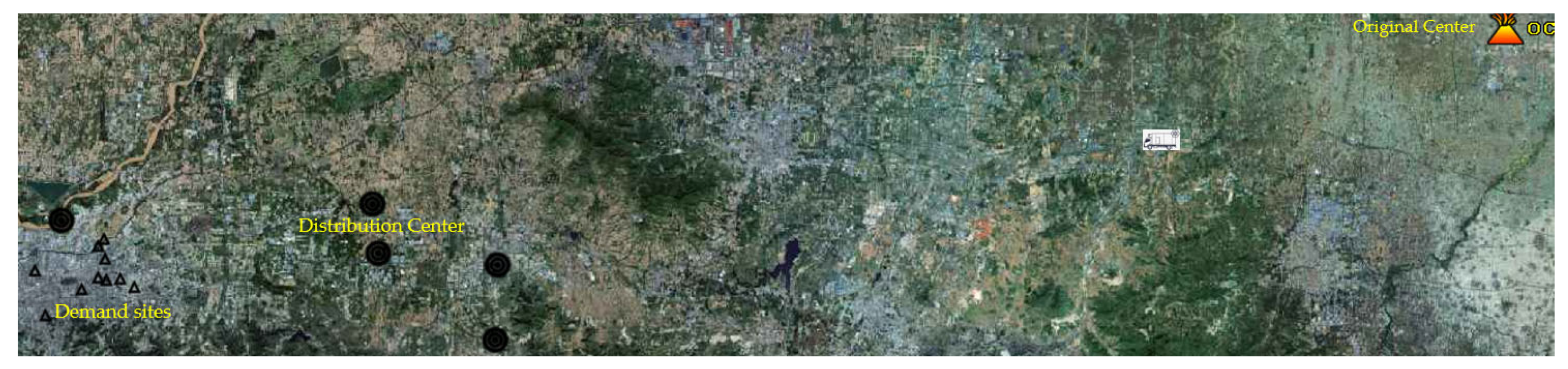
3. Problem Description

3.1. Problem Description

In the context of carbon neutrality goals, higher requirements have been posed for the innovation of agricultural transportation scheduling. We have considered the production, transportation, and distribution systems of fresh agricultural products, including multiple origin centers (pastures or farms), multiple distribution centers, and multiple demand sites. Fresh agricultural product transportation companies transfer fresh agricultural products through transportation (trucks) and transport them to demand sites (see Figure 1). Affected by the particularity of agricultural products, during the transportation of fresh agricultural products the number of agricultural products arriving is reduced due to the problem of decay. In the process of transportation, the potential decay of fresh food should be considered so that the initial transportation quantity should be increased. Fresh agricultural products finally arrive at the demand site for sale. In terms of traffic scheduling planning, how to effectively avoid risks and improve benefits is a hot research topic at present. At the same time, our research has also promoted the implementation of carbon neutrality goals.

3.2. Assumptions

According to the feasibility and scientific nature of mathematical modeling, this section proposes the following basic assumptions:

◆

It is assumed that logistics transportation is one-way transportation [30], that is, the direction is from the origin to the demand place;

◆

All agricultural products supplied are from the origin sites, and there is no input from outside the industrial chain [31];

◆

Transport vehicles of the same model (fuel consumption and capacity) are used in the same phase;

◆

Know the location of candidate demand sites in advance [32];

◆

The speed of the vehicle varies depending on the actual situation [33].

4. Model

4.1. Mixed Integer Linear Programming Model

In this section, the routing planning of the fresh agricultural products transportation network is modeled and analyzed. Considering the various costs in the research problem comprehensively, namely the fixed cost of distribution centers, configuration cost of vehicles, transportation cost, and time windows cost, a mixed integer linear programming model (MILP) model is constructed. The objective is to minimize the total cost, as shown in Formula (1).

$$\underset{x_i\in X,y_{ij}\in Y}{\mathrm{minimize}}\left\{\begin{array}{l}{\displaystyle {\sum }_{i\in I}{c}_i^f{x}_i}+{\displaystyle {\sum }_{i\in I}{c}_i^n{n}_i}+{\displaystyle {\sum }_{i\in I}{\displaystyle {\sum }_{j\in J}{c}_{ij}^v{d}_{ij}⌈\frac{y_{ij}{q}_j}{h_v(1-\tau )}⌉}}\\ +{\displaystyle {\sum }_{i\in I}{\displaystyle {\sum }_{j\in J}{y}_{ij}{c}_{ij}^t{\{\frac{d_{ij}}{v_{ij}}+w_{ij}-t_0,0\}}^{+}}}+{\displaystyle {\sum }_{i\in I}{\displaystyle {\sum }_{j\in J}{c}_{ij}^e{E}_{ij}^e{d}_{ij}{n}_i}}\end{array}\right\}$$

(1)

Subject to,

$$s.t.{\displaystyle {\sum }_{i\in I}{x}_i}\le \left|I\right|$$

(2)

$$y_{ij}\le M{x}_i,\forall i\in I$$

(3)

$$t_j^l\le t_i+y_{ij}{d}_{ij}{v}_{ij}{}^{-1}+w_{ij}\le t_{ij}^u,\forall i\in I,\forall j\in J$$

(4)

$${\displaystyle {\sum }_{i\in I}{y}_{ij}}=1,\forall j\in J$$

(5)

$${\displaystyle {\sum }_{j\in J}\frac{y_{ij}{q}_j}{1-\upsilon }}\le n_i{h}_v,\forall i\in I$$

(6)

$$n_i{h}_v\le H_i^{\max },\forall i\in I$$

(7)

$${\displaystyle {\sum }_{i\in I}{E}_e{d}_{ij}{n}_i}\le e^{\max },\forall j\in J$$

(8)

$$⌈y_{ij}⌉d_{ij}\le d^{\max },\forall i\in I,\forall j\in J$$

(9)

$$x_i\in \{0,1\},n_i\in \{0,1,\dots ,N\},y_{ij}\in [0,1],\forall i\in I,\forall j\in J$$

(10)

The relevant constraints are explained as follows. Constraint (2) is the quantity constraint of available distribution centers. Constraint (3) means that the premise of the routing planning decision is that the distribution center is selected [34,35]. Constraint (4) is a time window constraint, and $t_j^l,t_j^u$ represents the minimum arrival time and the maximum arrival time, respectively [36,37]. Constraint (5) means that the demand of any demand station must be met. Constraint (6) indicates that the actual transportation volume is lower than the rated transportation volume. Constraint (7) is the inventory constraint of the distribution center. Constraint (8) refers to carbon emission constraints, and the cumulative carbon emissions are strictly limited by carbon-neutral policies. Constraint (9) is the maximum mileage constraint for the truck. Constraint (10) represents constraints on related decision variables.

4.2. Interval Robust Counterpart Model

The complete information scenario is the most ideal scenario in theoretical research. On the contrary, the external environment of the market is full of uncertainty, so there is no ideal scenario in real life [38]. There are great uncertainties in the transportation of green agricultural products, especially the uncertainty of demand and the uncertainty of supply. Many scholars use robust optimization theories and methods to resist the influence of uncertain factors [39,40,41] and verify the feasibility of the robust model through multiple dimensions [42,43,44], citing the research ideas of relevant scholars [45,46,47] to expand the demand uncertainty in the transportation of green agricultural products.

Proposition 1.

Introduce a robust optimization theory to define uncertain parameter sets ${\mathrm{U}}_I$, the transformation from deterministic to uncertain parameters can be realized, then the objective function $\underset{x_i\in X,y_{ij}\in Y}{\mathrm{minimize}}\left\{F(x_i,y_{ij})|q_j\right\}$in the deterministic model can be transformed into$\underset{x_i\in X,y_{ij}\in Y,{\epsilon }_j\in U_I}{\mathrm{minimize}}\left\{F(x_i,y_{ij}|q_j^0,{\epsilon }_j\Delta )\right\}$in Equation(11) of the interval robust counterpart (IRC) model, with the constraints (6) in the MILP model relaxed to ${\displaystyle {\sum }_{j\in J}\frac{y_{ij}{q}_j^0}{1-\tau }}+\mathsf{\Psi }\underset{{\epsilon }_j\in U_I}{\sup }{\displaystyle {\sum }_{j\in J}{c}_v{d}_{ij}⌈\frac{y_{ij}{\epsilon }_j\Delta }{1-\tau }⌉}\le n_i{h}_v,\forall i\in I$.

Proof of Proposition 1.

The complete information situation is further transformed into an incomplete information situation, and the deterministic MILP model is transformed into a robust model, the goal of which is to pursue total cost minimization under the condition of incomplete information. Based on the basic MILP model, which $q_j$ under the complete information scenario defines the interval value uncertainty set $U_I$, which is $\left\{{\tilde{q}}_j\in {ℝ}^n,{\tilde{q}}_j=q_j^0+{\epsilon }_j\Delta ,{\epsilon }_j\in [a,b],{\displaystyle {\sum }_{j\in J}{\epsilon }_j\le \mathsf{\Psi },\forall j}\right\}$, where $q_j^0$ is the nominal value, $\Delta$ is the benchmark floating quantity, and ${\epsilon }_j$ is the uncertain parameter. Only the floating interval $[a,b]$ is known but the specific probability distribution is not known and $\mathsf{\Psi }$ is a safety parameter indicating the amount of uncertainty, so we made $q_j\to {\tilde{q}}_j$. Then, the related constraints are further relaxed to meet the constraints of real resource constraints. Among them, the constraint ${\displaystyle {\sum }_{j\in J}\frac{y_{ij}{q}_j}{1-\upsilon }}\le n_i{h}_v,\forall i\in I$ in the MILP model, the relaxation is as Equation (16). Similarly, $q_j\to {\tilde{q}}_j$ is also replaced in the objective function, and the objective function is also transformed into a robust problem in an uncertain parameter environment. To simplify the expression, let $F_0(y_{ij}|q_j^0)$ and $F^{\prime }[y_{ij},{\epsilon }_j,\Delta ]$ represent the expressions of objective functions for deterministic and uncertain scenarios, respectively. Among them, ${\displaystyle {\sum }_{i\in I}{\displaystyle {\sum }_{j\in J}{c}_{ij}^v{d}_{ij}⌈\frac{y_{ij}{q}_j}{h_v(1-\tau )}⌉}}$ is transferred to $\mathsf{\Psi }\underset{{\epsilon }_j\in U_I}{\sup }{\displaystyle {\sum }_{i\in I}{\displaystyle {\sum }_{j\in J}{c}_v{d}_{ij}⌈\frac{y_{ij}{\tilde{q}}_j}{h_v(1-\tau )}⌉}},{\tilde{q}}_j:=q_j^0+{\epsilon }_j\Delta$. The objective function is disassembled ${\tilde{q}}_j\to q_j^0+{\epsilon }_j\Delta ,{\epsilon }_j\in U_I$ to obtain the objective under the uncertain situation with safety parameters, as shown in (11), which is $\underset{x_i\in X,y_{ij}\in Y,{\epsilon }_j\in U_I}{\mathrm{minimize}}\left\{F(x_i,y_{ij}|q_j^0,{\epsilon }_j\Delta )\right\}$. □

The objective function (11) of the IRC model is to minimize the total cost.

$$\underset{x_i\in X,y_{ij}\in Y}{\mathrm{minimize}}\left\{\begin{array}{l}{\displaystyle {\sum }_{i\in I}{c}_i^f{x}_i}+{\displaystyle {\sum }_{i\in I}{c}_i^n{n}_i}+{\displaystyle {\sum }_{i\in I}{\displaystyle {\sum }_{j\in J}{y}_{ij}{c}_{ij}^t{\{\frac{d_{ij}}{v_{ij}}+w_{ij}-t_0,0\}}^{+}}}\\ +{\displaystyle {\sum }_{i\in I}{\displaystyle {\sum }_{j\in J}{c}_{ij}^e{E}_{ij}^e{d}_{ij}{n}_i}}+{\displaystyle {\sum }_{i\in I}{\displaystyle {\sum }_{j\in J}{c}_{ij}^v{d}_{ij}⌈\frac{y_{ij}{q}_j^0}{h_v(1-\tau )}⌉}}\\ +\mathsf{\Psi }\underset{{\epsilon }_j\in U_I}{\sup }{\displaystyle {\sum }_{i\in I}{\displaystyle {\sum }_{j\in J}{c}_{ij}^v{d}_{ij}⌈\frac{y_{ij}{\epsilon }_j\Delta }{h_v(1-\tau )}⌉}}\end{array}\right\}$$

(11)

Subject to,

Constraints (2), (3), (4), (5)

$${\displaystyle {\sum }_{j\in J}\frac{y_{ij}{q}_j^0}{1-\tau }}+\mathsf{\Psi }\underset{{\epsilon }_j\in U_I}{\sup }{\displaystyle {\sum }_{j\in J}{c}_v{d}_{ij}⌈\frac{y_{ij}{\epsilon }_j\Delta }{1-\tau }⌉}\le n_i{h}_v,\forall i\in I$$

(12)

Constraints (7), (8), (9), (10)

Interpretations of the relevant constraints of the IRC model are as follows. Constraints (2)–(5) have the same meaning in the MILP model. They are quantity constraints of distribution centers, association constraints of routes and distribution centers, time windows constraints, and demand satisfaction constraints. Constraint (16) indicates that the actual traffic volume under uncertain conditions is lower than the rated traffic volume constraint. The meaning of constraint (7)–(10) is the same as in the MILP model.

4.3. Ellipsoid Robust Counterpart Model

In addition to interval uncertainty sets, ellipsoidal uncertainty sets are also commonly used tools to characterize uncertain parameters. In this section, we build the ellipsoidal robust counterpart (ERC) model.

Proposition 2.

Introduce a robust optimization theory to define an ellipsoid uncertainty set${\mathrm{U}}_E$, which can realize the transformation of deterministic parameters to uncertain parameters, then the objective function$\underset{x_i\in X,y_{ij}\in Y}{\mathrm{minimize}}\left\{x_i,y_{ij}|q_j\right\}$in the MILP model can be converted to$\underset{x_i\in X,y_{ij}\in Y,{\xi }_j\in U_E}{\mathrm{minimize}}\left\{F(x_i,y_{ij}|q_j^0,{\xi }_j)\right\}$$\underset{x_i\in X,y_{ij}\in Y}{\text{minimize}}\left\{G_0\left(xi,yij\right)+G_0\left(xi,yij|q_j^0\right)+\mathsf{\Omega }\underset{\xi j\in UE}{\sup }{G}^{\prime }\left(xi,yij|\xi j\right)\right\}$in the ERC model, with the constraints (6) in the MILP model will be relaxed to${\displaystyle {\sum }_{i\in I}{\displaystyle {\sum }_{j\in J}{c}_{ij}^v{d}_{ij}⌈\frac{y_{ij}{q}_j^0}{h_v(1-\tau )}⌉}}+\mathsf{\Omega }\underset{{\xi }_j\in U_E}{\sup }\sqrt{{\displaystyle {\sum }_{i\in I}{\displaystyle {\sum }_{j\in J}{\left(c_{ij}^v{d}_{ij}⌈\frac{y_{ij}{\epsilon }_j\Delta }{h_v(1-\tau )}⌉\right)}^2}}}$.

Proof of Proposition 2.

The complete information scenario is extended to the incomplete information scenario, and the demand parameters are expanded, represented by $q_j$ [48,49]. The basic MILP model is further transformed into the ERC model, where the ellipsoid set is defined as the ${\mathrm{U}}_E=\left\{{\tilde{q}}_j\in {ℝ}^n,q_j:=q_j^0+\xi \Delta ,‖\xi ‖\le \mathsf{\Omega }\right\}$ uncertainty parameter covariance satisfying $\left\{q_j\in {ℝ}^n,{(q_j-q_j^0)}^T{\mathsf{\Sigma }}^{-1}(q_j-q_j^0)\le {\mathsf{\Omega }}^2\right\}$, where $q_j^0$ is a nominal value, $\Delta ={\mathsf{\Sigma }}^{\frac{1}{2}}$, $\mathsf{\Sigma }$ is a positive definite matrix, and $\mathsf{\Omega }$ is a safety parameter indicating the amount of uncertainty. By using an affine transformation, it can also be expressed as a ball of radius $\mathsf{\Omega }$. Considering $q_j\to {\tilde{q}}_j$, the constraints associated with it are further relaxed to satisfy the constraint constraints, where ${\displaystyle {\sum }_{j\in J}\frac{y_{ij}{q}_j}{1-\upsilon }}\le n_i{h}_v$ is constrained, which is relaxing as ${\displaystyle {\sum }_{j\in J}\frac{y_{ij}{q}_j^0}{1-\tau }}+\mathsf{\Omega }\underset{{\xi }_j\in U_E}{\sup }\sqrt{{\displaystyle {\sum }_{j\in J}{\left(c_v{d}_{ij}⌈\frac{y_{ij}{\xi }_j\Delta }{1-\tau }⌉\right)}^2}}\le n_i{h}_v$. Similarly, we let $q_j\to {\tilde{q}}_j$ be replaced in the objective function, and the objective function is also transformed accordingly. To simplify the expression, set $G_0(x_i,y_{ij})={\displaystyle {\sum }_{i\in I}{c}_i^f{x}_i}+{\displaystyle {\sum }_{i\in I}{c}_i^n{n}_i}+{\displaystyle {\sum }_{i\in I}{\displaystyle {\sum }_{j\in J}{y}_{ij}{c}_{ij}^t{\{\frac{d_{ij}}{v_{ij}}+w_{ij}-t_0,0\}}^{+}}}$ and $G(y_{ij},q_j^0)={\displaystyle {\sum }_{i\in I}{\displaystyle {\sum }_{j\in J}{c}_{ij}^e{E}_{ij}^e{d}_{ij}{n}_i}}+{\displaystyle {\sum }_{i\in I}{\displaystyle {\sum }_{j\in J}{c}_{ij}^v{d}_{ij}⌈\frac{y_{ij}{q}_j^0}{h_v(1-\tau )}⌉}}$ and consider the robustness of the objective function $\sqrt{{\displaystyle {\sum }_{i\in I}{\displaystyle {\sum }_{j\in J}{\left(c_{ij}^v{d}_{ij}⌈\frac{y_{ij}{\xi }_j\Delta }{h_v(1-\tau )}⌉\right)}^2}}}\le \mathsf{\Omega }\underset{{\xi }_j\in {\mathbb{U}}_E}{\sup }{G}^{\prime }(x_i,y_{ij}|{\xi }_j\Delta )$, to represent the optimal strategy under the worst case, $\underset{x_i\in X,y_{ij}\in Y}{\mathrm{minimize}}\left\{F(x_i,y_{ij})\right\}$ that is changed to $\underset{x_i\in X,y_{ij}\in Y,{\xi }_j\in U_E}{\mathrm{minimize}}\left\{F(x_i,y_{ij}|q_j^0,{\xi }_j)\right\}$ $\underset{x_i\in X,y_{ij}\in Y}{\text{minimize}}\left\{G_0\left(xi,yij\right)+G_0\left(xi,yij|q_j^0\right)+\mathsf{\Omega }\underset{\xi j\in UE}{\sup }{G}^{\prime }\left(xi,yij|\xi j\right)\right\}$. □

The objective function of the ERC model is to minimize the total cost (13).

$$\underset{x_i\in X,y_{ij}\in Y}{\text{minimize}}\left\{\begin{array}{l}{\displaystyle {\sum }_{i\in I}{c}_i^f{x}_i}+{\displaystyle {\sum }_{i\in I}{c}_i^n{n}_i}+{\displaystyle {\sum }_{i\in I}{\displaystyle {\sum }_{j\in J}{y}_{ij}{c}_{ij}^t{\{\frac{d_{ij}}{v_{ij}}+w_{ij}-t_0,0\}}^{+}}}\\ +{\displaystyle {\sum }_{i\in I}{\displaystyle {\sum }_{j\in J}{c}_{ij}^e{E}_{ij}^e{d}_{ij}{n}_i}}+{\displaystyle {\sum }_{i\in I}{\displaystyle {\sum }_{j\in J}{c}_{ij}^v{d}_{ij}⌈\frac{y_{ij}{q}_j^0}{h_v(1-\tau )}⌉}}\\ +\mathsf{\Omega }\underset{{\xi }_j\in U_E}{\sup }\sqrt{{\displaystyle {\sum }_{i\in I}{\displaystyle {\sum }_{j\in J}{\left(c_{ij}^v{d}_{ij}⌈\frac{y_{ij}{\epsilon }_j\Delta }{h_v(1-\tau )}⌉\right)}^2}}}\end{array}\right\}$$

(13)

Subject to,

Constraints (2), (3), (4), (5)

$${\displaystyle {\sum }_{j\in J}\frac{y_{ij}{q}_j^0}{1-\tau }}+\mathsf{\Omega }\underset{{\xi }_j\in U_E}{\sup }\sqrt{{\displaystyle {\sum }_{j\in J}{\left(c_v{d}_{ij}⌈\frac{y_{ij}{\xi }_j\Delta }{1-\tau }⌉\right)}^2}}\le n_i{h}_v,\forall i\in I$$

(14)

Constraints (7), (8), (9), (10)

Interpretations of the relevant constraints are as follows. Constraints (2)–(5) in the ERC model mean the same as those in the MILP model, which are, respectively, the quantity constraints of distribution centers, routing and distribution center association constraints, time windows, and demand satisfaction constraints. The constraint (14) indicates that the actual traffic volume under uncertain parameters is lower than the rated traffic volume constraint. The meaning of constraint (7)–(10) is the same as in the MILP model.

5. Data and Algorithm

In this section, we will verify the effectiveness of the proposed model and theory in real scenes. A transportation enterprise located in the famous vegetable production base in Shouguang, Shandong Province, was selected as the case study object. Vegetables are famous for their high level of industrialization, large area, high yield, high quality, and complete varieties [50]. This paper studies an agricultural production and marketing enterprise, which is engaged in the production and marketing operation services of agricultural products. The specific process is to purchase agricultural products from the original center (OC), transfer them through the transit distribution center (DC), and transport them to the target demand site (DS). The specific form is shown in Figure 2. The production base uses new production technology and advanced production equipment, which can not only produce high-quality organic products but also realize the off-season production of some vegetables, which can be continuously distributed to the distribution. The department supplies fresh produce. The selection of candidate transit warehouses refers to a variety of criteria, including the accessibility of the traffic location, whether the equipment meets the standard, whether the warehouse capacity meets the demand, and the economy. Through comprehensive screening, five candidate warehouses were finally determined, which were marked with symbol circles. The demand site is the supermarket closest to the user. These supermarkets are densely distributed on the main roads and traffic-intensive areas of the city, respectively.

The contents of this section are outlined below. Section 5.1 introduces the source and data structure of the data used in this case. Section 5.2 designs a solver-based solution algorithm framework.

5.1. Data

The basic data information involves refrigerated transfer stations, refrigerated trucks, and demand sites. The data comes from field research [51,52], as shown in

Table 2. Refrigerated truck parameters.

Item	Data
The load of transportation tools	1000–1500 kg
The unit energy consumption	25 L
The maximum speed limit	60 km/h
The average speed	30–45 km/h

and

Table 3. Data of the distribution center.

The Distribution Center	$\mathit{D}{\mathit{C}}_1$	$\mathit{D}{\mathit{C}}_2$	$\mathit{D}{\mathit{C}}_3$	$\mathit{D}{\mathit{C}}_4$	$\mathit{D}{\mathit{C}}_5$
The fixed cost	15,000 CNY	20,000 CNY	10,000 CNY	20,000 CNY	20,000 CNY
The maximum stock	9000 kg	7000 kg	8000 kg	6000 kg	6000 kg
Longitude (E)	117.019473	117.531636	117.5187	117.388586	117.391322
Latitude (N)	36.719945	36.678218	36.882706	36.690375	36.740998
The demand site	$D{s}_1$	$D{s}_2$	$D{s}_3$	$D{s}_4$	$D{s}_5$
The nominal demand	2000 kg	3500 kg	4000 kg	2500 kg	3000 kg
The demand site	$D{s}_6$	$D{s}_7$	$D{s}_8$	$D{s}_9$	$D{s}_{10}$
The nominal demand	2500 kg	3000 kg	4500 kg	3000 kg	3500 kg

. The actual distance between two sites can be directly obtained from Google Maps with web crawling technology, as shown in

Table 4. Distance.

	$\mathit{D}{\mathit{C}}_1$	$\mathit{D}{\mathit{C}}_2$	$\mathit{D}{\mathit{C}}_3$	$\mathit{D}{\mathit{C}}_4$	$\mathit{D}{\mathit{C}}_5$
$D{s}_1$	16.4 km	11.2 km	10.8 km	7.2 km	13.9 km
$D{s}_2$	39.9 km	62.3 km	60.9 km	57.1 km	58.2 km
$D{s}_3$	52.2 km	54.4 km	53.3 km	59.7 km	55.2 km
$D{s}_4$	66.8 km	60.4 km	57.9 km	56.6 km	56.1 km
$D{s}_5$	36.1 km	50.1 km	36.1 km	32.2 km	45.3 km
$D{s}_6$	7.8 km	11.7 km	12.3 km	10.4 km	8.5 km
$D{s}_7$	58.7 km	41.9 km	62.4 km	60.5 km	58.5 km
$D{s}_8$	64.2 km	51.1 km	53.2 km	53.1 km	56.5 km
$D{s}_9$	50.5 km	62.2 km	59.2 km	60.8 km	56.4 km
$D{s}_{10}$	41.2 km	36.9 km	37.5 km	35.6 km	33.5 km

.

5.2. Algorithm

Based on the above basic data values, this section uses Python as the programming platform to design the solution framework, and calls the solver Gurobi (9.5) to solve the MILP, ERC, and IRC models. To ensure the scientificity of the case, the control variable method is used for verification, and the same environment (Windows 10, Intel (R) Core (TM) i5-8300H, HP, USA) is used on the same computer [email protected] GHz, RAM8 GB, 512 G SSD).

The Benders decomposition algorithm has been widely used in various optimization problems [53,54,55]. In order to solve the problem of routing planning for large-scale fresh agricultural products, we will build a solution framework based on Gurobi in this section. However, algorithms based on solvers often require high-standard forms of models and are difficult to solve large-scale computing problems. To effectively deal with non-standard model optimization problems, we develop a customized Benders decomposition algorithm to solve them. Firstly, we separate the original problem into a subproblem. Then, we solve the subproblem to obtain the initial feasible solution. Secondly, we trace the initial feasible solution of the subproblem back to the main problem and further construct the overall optimization model considering the relevant constraints of the main problem. Thirdly, in order to improve the efficiency of the model, we adjust the constraints in the model that are difficult to solve directly by adding optimal cuts or feasible cuts to Farkas‘ lemma [56]. Finally, we derive the optimal or feasible solution of the model. The overall framework of our improved algorithm is shown in Algorithm 1.

Algorithm 1. Benders decomposition algorithm

$\mathrm{Input} \mathrm{nominal} \mathrm{parameters} : c_i^f,c_{ij}^v,c_{ij}^t,c_{ij}^e,d_{ij},q_j,h_v,\tau ,v_{ij},w_{ij},t_0,E_{ij}^e$

$\mathrm{Initialization} \mathrm{boundary}:(LB:=-\infty ,UB:=+\infty )$$, \mathrm{Set} (I,J)$

1 Identify Master problem $\{\mathrm{MP}, F(x_i,n_i|y_{ij})\}$, Sub-problem $\{\mathrm{SP},F(y_{ij})\}$

2 Repeat $n\leftarrow 1$

3  for MILP model, $q_j\leftarrow q_j$

4  for IRC model, $q_j\leftarrow q_j^0+{\epsilon }_j\Delta ,{\epsilon }_j\in U_I$

5  for ERC model, $q_j\leftarrow q_j^0+{\xi }_j\Delta ,{\xi }_j\in U_E$

6  SP $\leftarrow$ Dual Sub-problem (DSP)

7    solving DSP by Gurobi get ${\mu }_{ij}^{*}$$( \mathrm{dual} \mathrm{variables} \mathrm{of} {\overline{y}}_{ij}^{}$) with constraints

8    if DSP is unbounded, add benders feasibility cut in MP

9     if $ob{j}^n{}_{DSP}<U{B}^{n+1},U{B}^{n+1}=ob{j}^n$

10     $\mathrm{else}, U{B}^{n+1}=U{B}^n$

11    if DSP is bounded, add benders optimality cut in MP

12     if $ob{j}^n{}_{DSP}<U{B}^{n+1},U{B}^{n+1}=ob{j}^n$

13     $\mathrm{else}, U{B}^{n+1}=+U{B}^n$

14     if no feasible solution for DSP

15     end

16 Obtain $x_i,n_i$ by solving MP

17    if $ob{j}^n{}_{MP}>L{B}^{n+1},L{B}^{n+1}=ob{j}^n$

18    else, $L{B}^{n+1}=L{B}^n$

19 $n\leftarrow n+1$

20 until ($\mathrm{Iterations}=\mathrm{n} \mathrm{or} UB-LB<\epsilon$)

Return value {$x_i^{*},n_i^{*},y_{ij}^{*}$}

6. Simulation

In Section 6.1 and Section 6.2, we analyze the impact of safety parameters and volatility. We present the routing planning scheme in Section 6.3. We compare the impact of carbon tax changes in Section 6.4. In Section 6.5, we compare the impact of changes in storage ratios across warehouses.

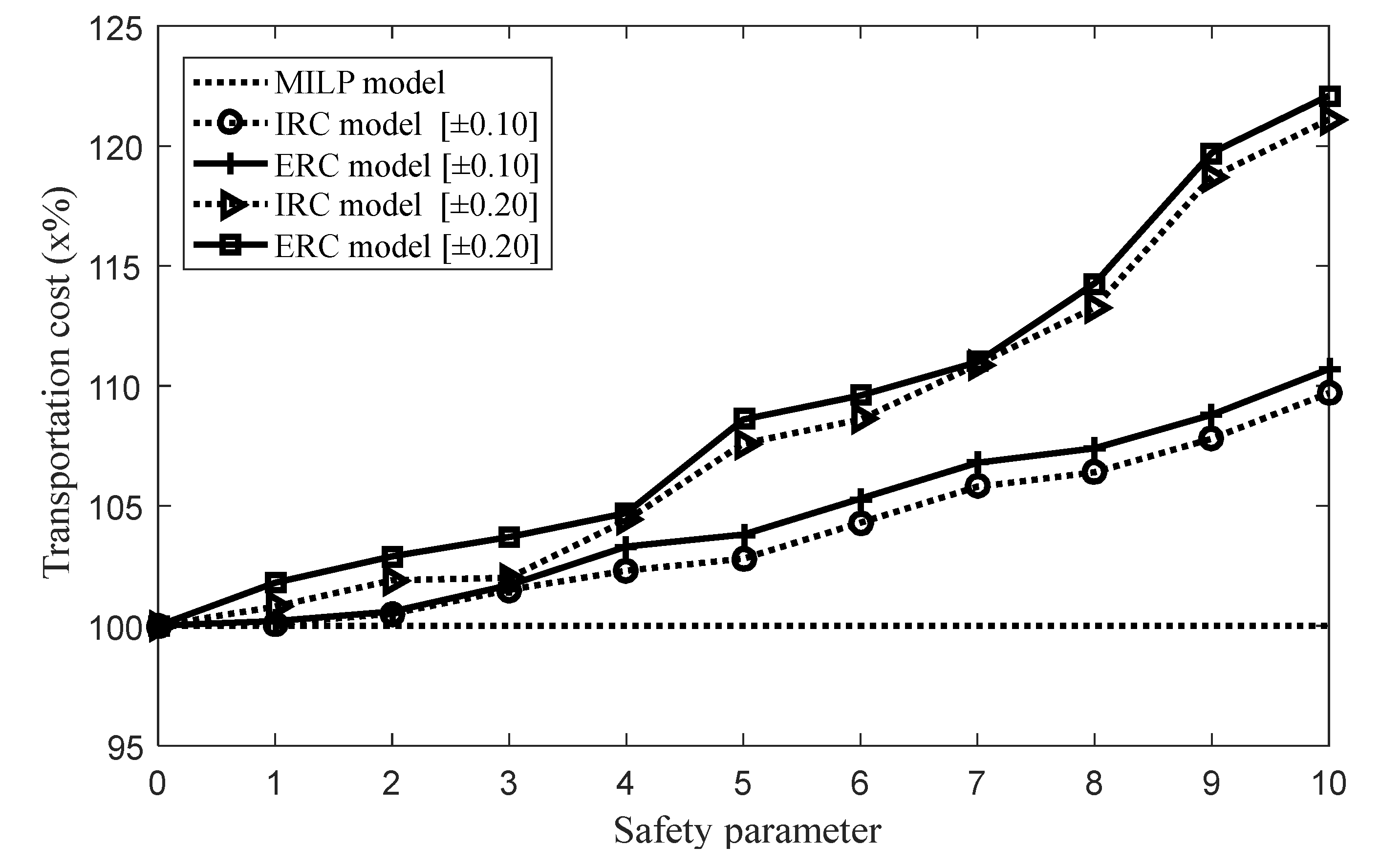
6.1. Influence of Safety Parameters

We compare the advantages of each model through cost response to safety parameters, as shown in Figure 3. The horizontal axis in the figure is a safety parameter, and the vertical axis is the total transportation cost. It can be seen that the MILP model has strong stability, and its total cost will not change with the change in security parameters. However, at the same time, there are also defects, that is, it is impossible to deal with planning problems in an uncertain environment. In the case of uncertain market parameters, both the IRC and ERC models can be obtained by feasible solutions but at the same time, the price of robust rots is required to resist the interference of uncertain parameters [57,58]. As the level of security parameters increases (that is, the uncertainty expansion), the total transportation costs show an upward trend. When the market is uncertain (SP = 10, all sites are disturbed by uncertain parameters), the maximum increase in total transportation costs is 20.1%, that is, the maximum cost increase in the worst scenario is 20.1%. In terms of the scope of the uncertain set, the larger the range of uncertain parameter fluctuations, ($\left[-0.10, 0.10\right]$ belongs to $\left[-0.20,0.20\right]$), the greater its transportation cost, whether it is an ERC or IRC model.

6.2. Influence of Volatility

We obtain the average value of the parameters by repeating the ERC and IRC models multiple times, and analyze the impact of uncertain parameters on the level of logistics services, as shown in Figure 4. The relevant parameter setting is as follows, and the horizontal axis represents the percentage of the amplitude of the uncertain parameter fluctuation. The vertical axis indicates the level of logistics service. The safety parameter level is 3, 5, 8, and 10, that is, the parameters of the maximum of 3, 5, 8, and 10 nodes may fluctuate. Compare the logistics service level of the MILP model as the reference (100%). Observe the impact of uncertain parameters on the level of logistics services.

It can be observed that the logistics service level of the robust model (the ERC and IRC models) is affected by the volatility of uncertain parameters. Overall, as the volatility of uncertain parameters increases, the level of the logistics service has shown a downward trend (the level of the service has decreased by 2.8%), which aligns with reality, and it is also confirmed in the research of scholars [59]. Another noteworthy phenomenon is that with the impact of the level of security parameters, the decline in the level of the logistics service levels has slowed down, and about 1.4% of the service level has declined. This discovery can provide guidance for corporate managers in their decision-making. In the case of the same parameter fluctuations, the use of higher security parameters will help improve the level of logistics services. In the same security parameter level, the greater the volatility of the parameter, the lower the level of logistics services. The accurate estimation of enterprises for demand parameters can better serve their retail companies and improve the comprehensive management level.

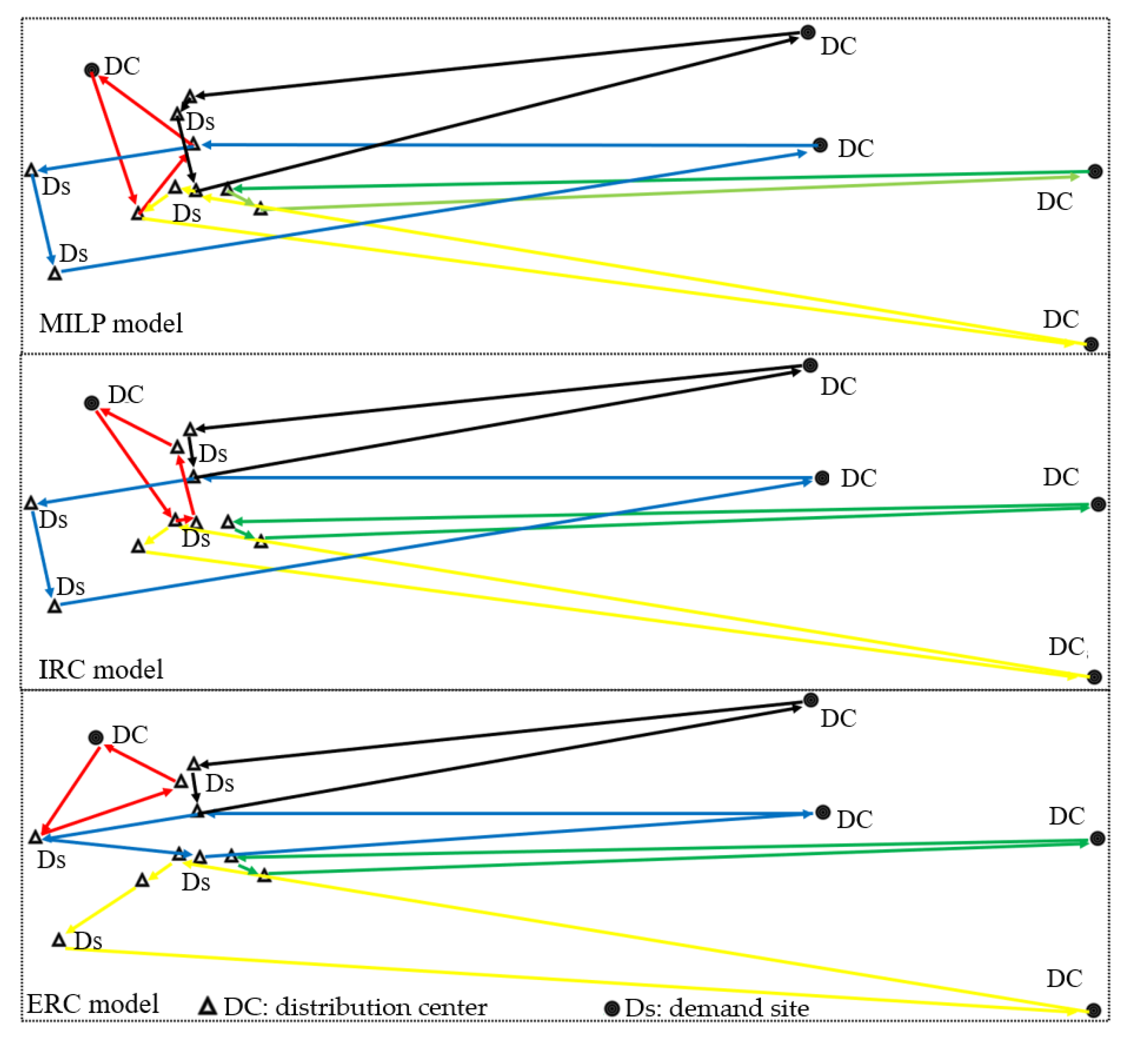
6.3. Routing Planning Design

Figure 5 depicts the planning and design scheme for the shipping of agricultural products from the origin center (OC) to the distribution center (DC). At this stage, agricultural products are transported in large quantities and with a single route. For direct transportation, large vehicles are generally used for transportation. Nodes with large storage levels at transit sites need to dispatch multiple vehicles to and from to complete transportation tasks. The relevant sites are described based on real maps.

The routing scheme of the MILP model, IRC model, and ERC model agricultural product distribution phase is shown in Figure 6. At this stage, agricultural products were transported from the distribution center (DC) to the demand site (Ds). The location of the node is fixed and definite. It can be seen from the figure that in the MILP model, there is a phenomenon of crossline and long-range transportation in the route planning scheme. The distribution routes of different distribution centers are marked with different colors. In other words, the overlapping transportation route means that extra transportation costs may be generated, causing a waste of transportation resources. This phenomenon also exists in the IRC model. In the ERC model’s solution, there are fewer route overlaps, which will make the transportation plan more reasonable and convenient, and it will help improve the effective allocation of transportation resources.

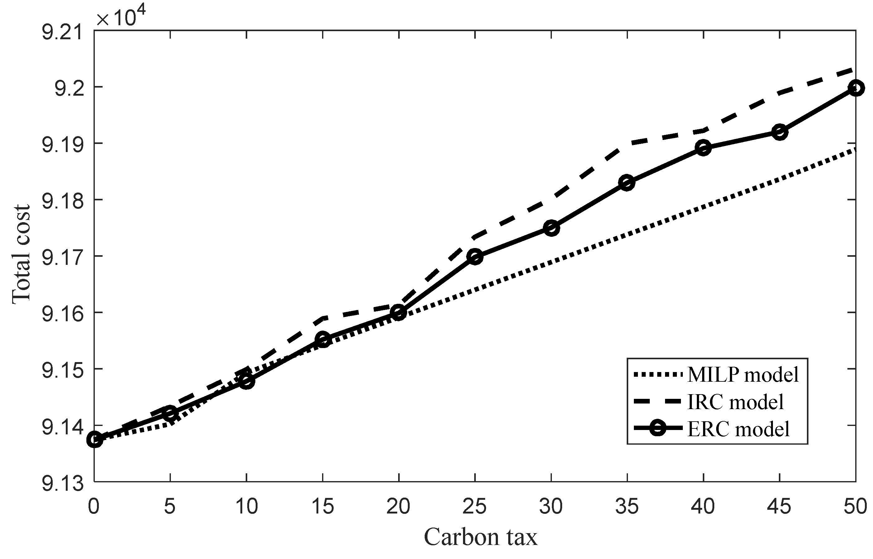
6.4. Impact of Carbon Tax Changes

Figure 7 is the responsiveness of each of the three models to changes in carbon taxes. Referring to real-world scenarios, we compare the MILP model, the IRC model, and the ERC model with carbon taxes varying from an interval of 0 to 50. It can be seen from the comparison that each model shows an upward trend with the increase of carbon tax. There is a slight difference in the comparison of details, among which, the cost increase in the IRC and ERC models is higher than the counterpart in the MILP model. Compared with the IRC model, the cost of the ERC model shows slighter increases, demonstrating the robustness of the ERC model. The increase in carbon tax costs will compel companies to adjust their transportation strategies to reduce costs by optimizing routes while meeting the requirements of environmental benefits.

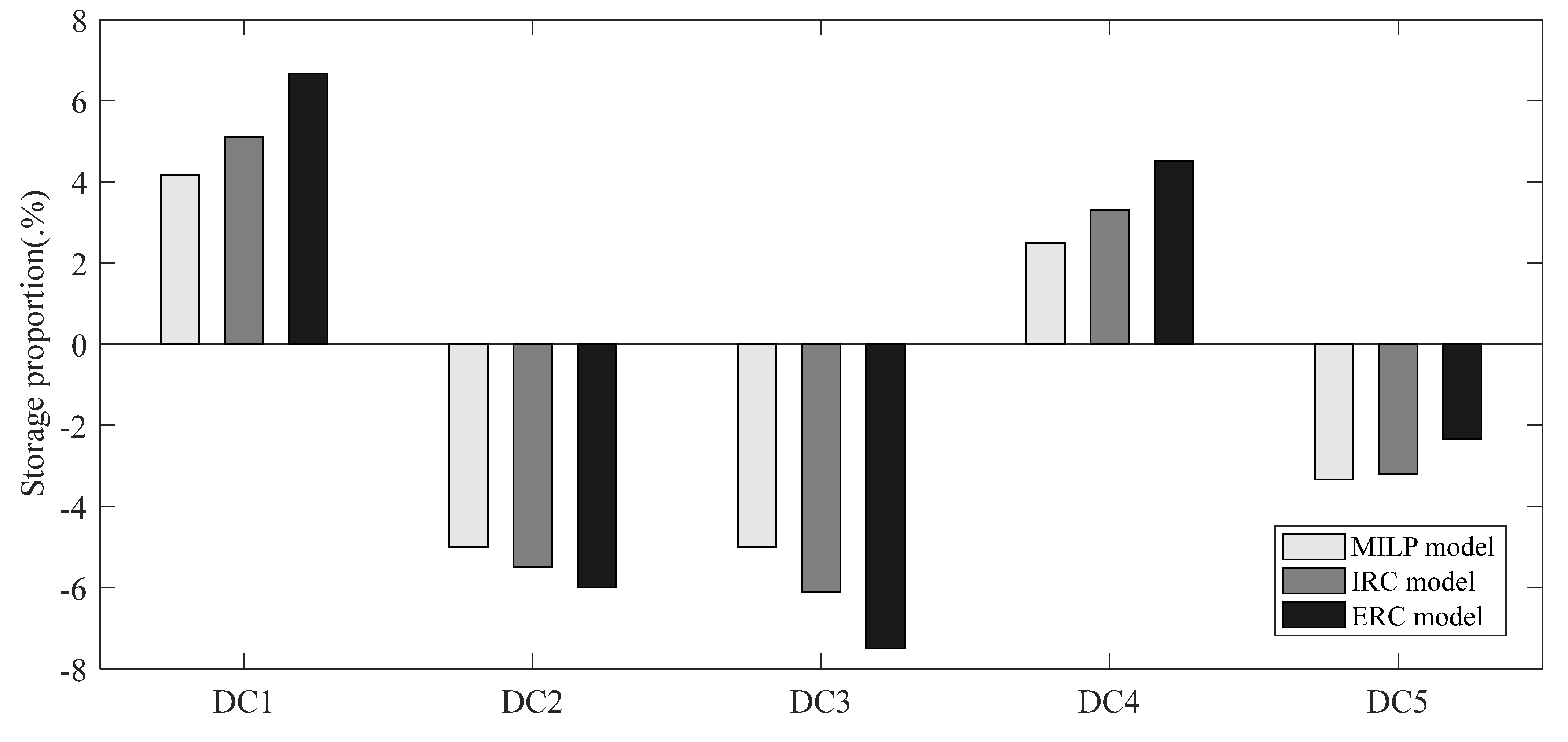
6.5. Storage Proportion of Distribution Center

Figure 8 depicts the storage proportion of distribution center. In order to compare the changes in the storage proportion of each model, the MILP model and the robust models are compared in this section. It can be seen that there are differences in each model. Among them, in the IRC and ERC models, the storage proportion at distribution centers DC1, DC4, and DC5 all present an upward trend, while distribution center DC2 and DC3 show a downward trend. Changes in the proportion of distribution center directly affect transportation costs and the quality of transportation services. The transportation plan can be effectively optimized by increasing the proportion of the distribution center method service close to the service demand point. In the actual enterprise management process, it provides guidance for the formulation of enterprise operation decision-making plans to some extent.

7. Conclusions

In this paper, a mixed integer linear programming model for the cold chain transportation of agricultural products that comprehensively considers various costs is proposed. The purpose is to study how to effectively reduce transportation costs and improve transportation efficiency in the parameter determination scenario. Uncertainty in the market environment is difficult to measure directly, which will lead to a rapid increase in transportation costs and unnecessary losses of agricultural products. Additionally, the parameters are extended to uncertain scenarios based on the mixed integer linear programming model, and a robust counterpart model based on uncertain parameter scenarios is proposed. A specific uncertainty robust set is constructed to characterize the fluctuation range of the uncertain parameters. Through the optimization model, the optimal strategy can be made in the worst case, so as to avoid the cost or loss due to increasing too fast. The guarantee of transportation is improved from the perspective of uncertainty optimization. Finally, the proposed model and traffic strategy are analyzed through a design case, the validity of the proposed model is verified, and management suggestions and traffic planning schemes are provided. The research reveals that the increase in carbon tax costs will compel companies to optimize their transportation route planning, improving their transportation efficiency. In addition, uncertain parameters will lead to a significant increase in cost, and accurate evaluation of demand parameters is essential in improving enterprise competitiveness.

However, there are some limitations to this study. First, the agricultural vehicle scheduling problem is analyzed only from the perspective of operations research optimization. In practical conditions, there are still many management problems that need to be further considered. Second, in the real world, there is inventory management under supply uncertainty scenarios due to climatic factors. Third, the multi-objective planning of the fresh agricultural products needs further research. Fourth, in different sales fields, there is the problem of precise rationing of heterogeneous consumer demand. Lastly, in the multimodal transport mode, there are complex scheduling and coordination problems, which have been rarely discussed in previous research and thus can be further researched in the future.

References

1. Chen, J.; Fan, T.; Pan, F. Urban delivery of fresh products with total deterioration value. Int. J. Prod. Res. 2021, 59, 2218–2228. [Google Scholar] [CrossRef]
2. De Oliveira, J.G.; Silva, G.D.; Cipriano, L.; Gomes, M.; Egea, M.B. Control of postharvest fungal diseases in fruits using external application of RNAi. J. Food Sci. 2021, 86, 3341–3348. [Google Scholar] [CrossRef] [PubMed]
3. Saif, A.; Elhedhli, S. Cold supply chain design with environmental considerations: A simulation-optimization approach. Eur. J. Oper. Res. 2016, 251, 274–287. [Google Scholar] [CrossRef]
4. Teng, S. Route planning method for cross-border e-commerce logistics of agricultural products based on recurrent neural network. Soft Comput. 2021, 25, 12107–12116. [Google Scholar] [CrossRef]
5. Hariga, M.; As’Ad, R.; Shamayleh, A. Integrated Economic and Environmental Models for a Multi Stage Cold Supply Chain under Carbon Tax Regulation. J. Clean. Prod. 2017, 166, 1357–1371. [Google Scholar] [CrossRef]
6. Evans, J.A.; Russell, S.L.; James, C.; Corry, J.E.L. Microbial contamination of food refrigeration equipment. J. Food Eng. 2004, 62, 225–232. [Google Scholar] [CrossRef]
7. Shishov, V.V.; Talyzin, M.S. Efficiency of Refrigeration Equipment on Natural Refrigerants. Chem. Pet. Eng. 2020, 56, 385–392. [Google Scholar] [CrossRef]
8. Melillo, J.M.; McGuire, A.D.; Kicklighter, D.W.; Moore, B.; Vorosmarty, C.J.; Schloss, A.L. Global climate change and terrestrial net primary production. Nature 1993, 363, 234–240. [Google Scholar] [CrossRef]
9. Johansson, B.; Hman, M. A comparison of technologies for carbon-neutral passenger transport. Transp. Res. Part D Transp. Environ. 2002, 7, 175–196. [Google Scholar] [CrossRef]
10. Krammer, P.; Dray, L.; Kohler, M.O. Climate-neutrality versus carbon-neutrality for aviation biofuel policy. Transp. Res. Part D-Transp. Environ. 2013, 23, 64–72. [Google Scholar] [CrossRef]
11. Liu, Z.; Deng, Z.; He, G.; Wang, H.L.; Zhang, X.; Lin, J.; Qi, Y.; Liang, X. Challenges and opportunities for carbon neutrality in China. Nat. Rev. Earth Environ. 2022, 3, 141–155. [Google Scholar] [CrossRef]
12. Ebrahimi, S.; Mac Kinnon, M.; Brouwer, J. California end-use electrification impacts on carbon neutrality and clean air. Appl. Energy 2018, 213, 435–449. [Google Scholar] [CrossRef]
13. Dulebenets, M.A.; Ozguven, E.E.; Moses, R.; Ulak, M.B. Intermodal freight network design for transport of perishable products. Open J. Optim. 2016, 5, 120. [Google Scholar] [CrossRef] [Green Version]
14. Theophilus, O.; Dulebenets, M.A.; Pasha, J.; Lau, Y.-Y.; Fathollahi-Fard, A.M.; Mazaheri, A. Truck scheduling optimization at a cold-chain cross-docking terminal with product perishability considerations. Comput. Ind. Eng. 2021, 156, 107240. [Google Scholar] [CrossRef]
15. Dulebenets, M.A.; Ozguven, E.E. Vessel scheduling in liner shipping: Modeling transport of perishable assets. Int. J. Prod. Econ. 2017, 184, 141–156. [Google Scholar] [CrossRef]
16. Zheng, F.; Pang, Y.; Xu, Y.; Liu, M. Heuristic algorithms for truck scheduling of cross-docking operations in cold-chain logistics. Int. J. Prod. Res. 2021, 59, 6579–6600. [Google Scholar] [CrossRef]
17. Qu, S.J.; Xu, L.; Mangla, S.K.; Chan, F.T.S.; Zhu, J.L.; Arisian, S. Matchmaking in reward-based crowdfunding platforms: A hybrid machine learning approach. Int. J. Prod. Res. 2022, 1–22. [Google Scholar] [CrossRef]
18. Feldmann, C.; Hamm, U. Consumers’ perceptions and preferences for local food: A review. Food Qual. Prefer. 2015, 40, 152–164. [Google Scholar] [CrossRef]
19. He, Q.Z.; Tong, H.; Liu, J.B. How Does Inequality Affect the Residents’ Subjective Well-Being: Inequality of Opportunity and Inequality of Effort. Front. Psychol. 2022, 13, 843854. [Google Scholar] [CrossRef]
20. Li, B.X.; Hu, H. Logistics Model Based on Agricultural Product Transportation. Agro Food Ind. Hi-Tech 2017, 28, 3370–3373. [Google Scholar]
21. Li, P.J. Logistics transportation route for agricultural products based on an improved ant colony algorithm. Agro Food Ind. Hi-Tech 2017, 28, 1876–1880. [Google Scholar]
22. Qi, C.; Hu, L. Optimization of vehicle routing problem for emergency cold chain logistics based on minimum loss. Phys. Commun. 2020, 40, 101085. [Google Scholar] [CrossRef]
23. Wang, M.; Cheng, Q.; Huang, J.C.; Cheng, G.Q. Research on optimal hub location of agricultural product transportation network based on hierarchical hub-and-spoke network model. Phys. A-Stat. Mech. Its Appl. 2021, 566, 125412. [Google Scholar] [CrossRef]
24. Khan, Z.A.; Koondhar, M.A.; Khan, I.; Ali, U.; Liu, T.J. Dynamic linkage between industrialization, energy consumption, carbon emission, and agricultural products export of Pakistan: An ARDL approach. Environ. Sci. Pollut. Res. 2021, 28, 43698–43710. [Google Scholar] [CrossRef] [PubMed]
25. Al-Mansour, F.; Jejcic, V. A model calculation of the carbon footprint of agricultural products: The case of Slovenia. Energy 2017, 136, 7–15. [Google Scholar] [CrossRef]
26. Sanye-Mengual, E.; Ceron-Palma, I.; Oliver-Sola, J.; Montero, J.I.; Rieradevall, J. Environmental analysis of the logistics of agricultural products from roof top greenhouses in Mediterranean urban areas. J. Sci. Food Agric. 2013, 93, 100–109. [Google Scholar] [CrossRef]
27. Zhu, S.J.; Fu, H.M.; Li, Y.H. Optimization Research on Vehicle Routing for Fresh Agricultural Products Based on the Investment of Freshness-Keeping Cost in the Distribution Process. Sustainability 2021, 13, 8110. [Google Scholar] [CrossRef]
28. Ahmed, W.; Sarkar, B. Management of next-generation energy using a triple bottom line approach under a supply chain framework. Resour. Conserv. Recycl. 2019, 150, 104431. [Google Scholar] [CrossRef]
29. Pan, F.; Fan, T.; Qi, X.; Chen, J.; Zhang, C. Truck scheduling for cross-docking of fresh produce with repeated loading. Math. Probl. Eng. 2021, 2021, 5592122. [Google Scholar] [CrossRef]
30. Drezner, Z.; Wesolowsky, G.O. Selecting an optimum configuration of one-way and two-way routes. Transp. Sci. 1997, 31, 386–394. [Google Scholar] [CrossRef]
31. Chen, J.; Gui, P.; Ding, T.; Na, S.; Zhou, Y. Optimization of transportation routing problem for fresh food by improved ant colony algorithm based on tabu search. Sustainability 2019, 11, 6584. [Google Scholar] [CrossRef] [Green Version]
32. Toole, J.L.; Colak, S.; Sturt, B.; Alexander, L.P.; Evsukoff, A.; González, M.C. The path most traveled: Travel demand estimation using big data resources. Transp. Res. Part C Emerg. Technol. 2015, 58, 162–177. [Google Scholar] [CrossRef]
33. Taghvaeeyan, S.; Rajamani, R. Portable roadside sensors for vehicle counting, classification, and speed measurement. IEEE Trans. Intell. Transp. Syst. 2013, 15, 73–83. [Google Scholar] [CrossRef]
34. Purba, D.S.D.; Kontou, E.; Vogiatzis, C. Evacuation route planning for alternative fuel vehicles. Transp. Res. Part C-Emerg. Technol. 2022, 143, 103837. [Google Scholar] [CrossRef]
35. Karak, A.; Abdelghany, K. The hybrid vehicle-drone routing problem for pick-up and delivery services. Transp. Res. Part C-Emerg. Technol. 2019, 102, 427–449. [Google Scholar] [CrossRef]
36. Schneider, M.; Stenger, A.; Goeke, D. The electric vehicle-routing problem with time windows and recharging stations. Transp. Sci. 2014, 48, 500–520. [Google Scholar] [CrossRef] [Green Version]
37. Jiang, L.; Dhiaf, M.; Dong, J.F.; Liang, C.Y.; Zhao, S.P. A traveling salesman problem with time windows for the last mile delivery in online shopping. Int. J. Prod. Res. 2020, 58, 5077–5088. [Google Scholar] [CrossRef]
38. Soyster, A.L.; Murphy, F.H. Data driven matrix uncertainty for robust linear programming. Omega-Int. J. Manag. Sci. 2017, 70, 43–57. [Google Scholar] [CrossRef]
39. Wiesemann, W.; Kuhn, D.; Sim, M. Distributionally Robust Convex Optimization. Oper. Res. 2014, 62, 1358–1376. [Google Scholar] [CrossRef] [Green Version]
40. Ji, Y.; Li, H.H.; Zhang, H.J. Risk-Averse Two-Stage Stochastic Minimum Cost Consensus Models with Asymmetric Adjustment Cost. Group Decis. Negot. 2022, 31, 261–291. [Google Scholar] [CrossRef]
41. Qu, S.J.; Wei, J.P.; Wang, Q.H.; Li, Y.M.; Jin, X.W.; Chaib, L. Robust minimum cost consensus models with various individual preference scenarios under unit adjustment cost uncertainty. Inf. Fusion 2023, 89, 510–526. [Google Scholar] [CrossRef]
42. Shi, Y.; Boudouh, T.; Grunder, O. A robust optimization for a home health care routing and scheduling problem with consideration of uncertain travel and service times. Transp. Res. Part E-Logist. Transp. Rev. 2019, 128, 52–95. [Google Scholar] [CrossRef]
43. Gorissen, B.L.; Yanıkoğlu, İ.; den Hertog, D. A practical guide to robust optimization. Omega 2015, 53, 124–137. [Google Scholar] [CrossRef] [Green Version]
44. Bai, D.; Carpenter, T.; Mulvey, J. Making a case for robust optimization models. Manag. Sci. 1997, 43, 895–907. [Google Scholar] [CrossRef]
45. Yu, C.-S.; Li, H.-L. A robust optimization model for stochastic logistic problems. Int. J. Prod. Econ. 2000, 64, 385–397. [Google Scholar] [CrossRef]
46. Baron, O.; Milner, J.; Naseraldin, H. Facility location: A robust optimization approach. Prod. Oper. Manag. 2011, 20, 772–785. [Google Scholar] [CrossRef]
47. Qu, S.; Li, Y.; Ji, Y. The mixed integer robust maximum expert consensus models for large-scale GDM under uncertainty circumstances. Appl. Soft Comput. 2021, 107, 107369. [Google Scholar] [CrossRef]
48. Matthews, L.R.; Guzman, Y.A.; Floudas, C.A. Generalized robust counterparts for constraints with bounded and unbounded uncertain parameters. Comput. Chem. Eng. 2018, 116, 451–467. [Google Scholar] [CrossRef]
49. Abdel-Aal, M.A.M.; Selim, S.Z. Robust optimization for selective newsvendor problem with uncertain demand. Comput. Ind. Eng. 2019, 135, 838–854. [Google Scholar] [CrossRef]
50. Liang, Z.; Wu, J.; Li, J.; Yang, Z.; Li, J.; Li, J. Application and Popularization of New Green Prevention and Control Technology for Greenhouse Vegetables in Shouguang City, Shandong Province. Asian Agric. Res. 2019, 11, 78–81. [Google Scholar]
51. Gao, J.; Wang, L.W.; Gao, P.; An, G.L.; Wang, Z.X.; Xu, S.Z.; Wang, R.Z. Performance investigation of a freezing system with novel multi-salt sorbent for refrigerated truck. Int. J. Refrig.-Rev. Int. Du Froid 2019, 98, 129–138. [Google Scholar] [CrossRef]
52. Romijn, T.C.J.; Donkers, M.C.F.; Kessels, J.; Weiland, S. A Distributed Optimization Approach for Complete Vehicle Energy Management. Ieee Trans. Control Syst. Technol. 2019, 27, 964–980. [Google Scholar] [CrossRef] [Green Version]
53. Rahmaniani, R.; Crainic, T.G.; Gendreau, M.; Rei, W. The Benders decomposition algorithm: A literature review. Eur. J. Oper. Res. 2017, 259, 801–817. [Google Scholar] [CrossRef]
54. Hooker, J.N.; Ottosson, G. Logic-based Benders decomposition. Math. Program. 2003, 96, 33–60. [Google Scholar] [CrossRef]
55. Hooker, J.N. Planning and scheduling by logic-based Benders decomposition. Oper. Res. 2007, 55, 588–602. [Google Scholar] [CrossRef] [Green Version]
56. Jeyakumar, V.; Lee, G.M. Complete characterizations of stable Farkas’ lemma and cone-convex programming duality. Math. Program. 2008, 114, 335–347. [Google Scholar] [CrossRef]
57. Zhang, X.; Ding, Z.J.; Hang, J.Q.; He, Q.Z. How do stock price indices absorb the COVID-19 pandemic shocks? N. Am. J. Econ. Financ. 2022, 60, 101672. [Google Scholar] [CrossRef]
58. Chen, Z.; Wu, L.; Fu, Y. Real-Time Price-Based Demand Response Management for Residential Appliances via Stochastic Optimization and Robust Optimization. Ieee Trans. Smart Grid 2012, 3, 1822–1831. [Google Scholar] [CrossRef]
59. Zhang, Z.-H.; Jiang, H. A robust counterpart approach to the bi-objective emergency medical service design problem. Appl. Math. Model. 2014, 38, 1033–1040. [Google Scholar] [CrossRef]
Figure 1. Transportation planning for fresh agricultural products.
Sustainability 14 14992 g001
Figure 2. Geographical location.
Sustainability 14 14992 g002
Figure 3. Influence of safety parameters.
Sustainability 14 14992 g003
Figure 4. The effect of volatility.
Sustainability 14 14992 g004
Figure 5. Route planning and design in the original stage.
Sustainability 14 14992 g005
Figure 6. The routing planning.
Sustainability 14 14992 g006
Figure 7. Impact of carbon tax changes.
Sustainability 14 14992 g007
Figure 8. Storage proportion at the distribution center.
Sustainability 14 14992 g008