

Atmospheric Anomalies Associated with the 2021 Mw 7.2 Haiti Earthquake Using Machine Learning from Multiple Satellites

 ,
,  ,
,  , ,
, ,
Abstract
1. Introduction
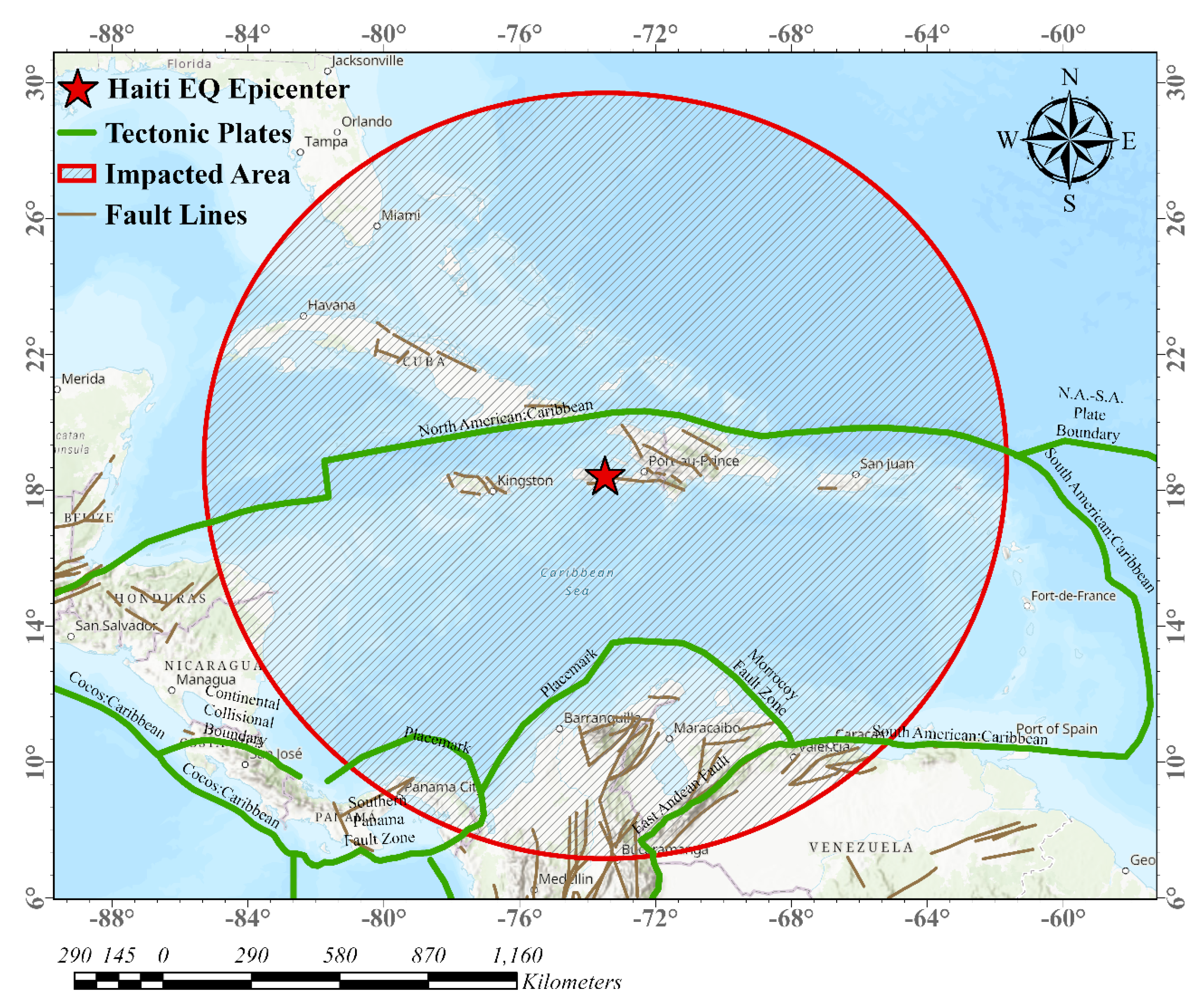
2. Study Area
3. Materials and Methods
3.1. Data Collection
3.2. Data Analysis
4. Results and Discussion
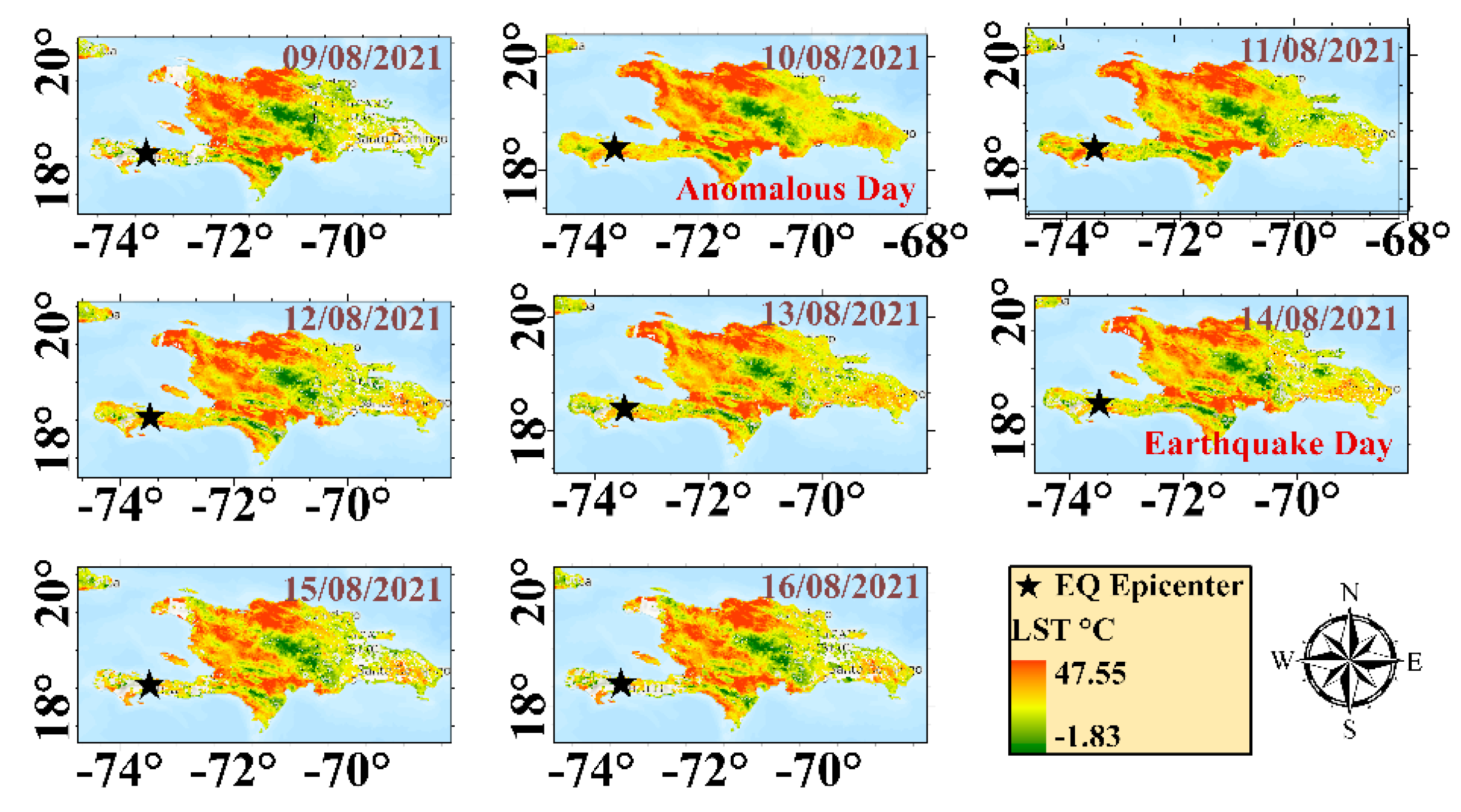
4.1. Anomalies Evidence
4.2. Possible Mechanism
5. Conclusions
- (1)
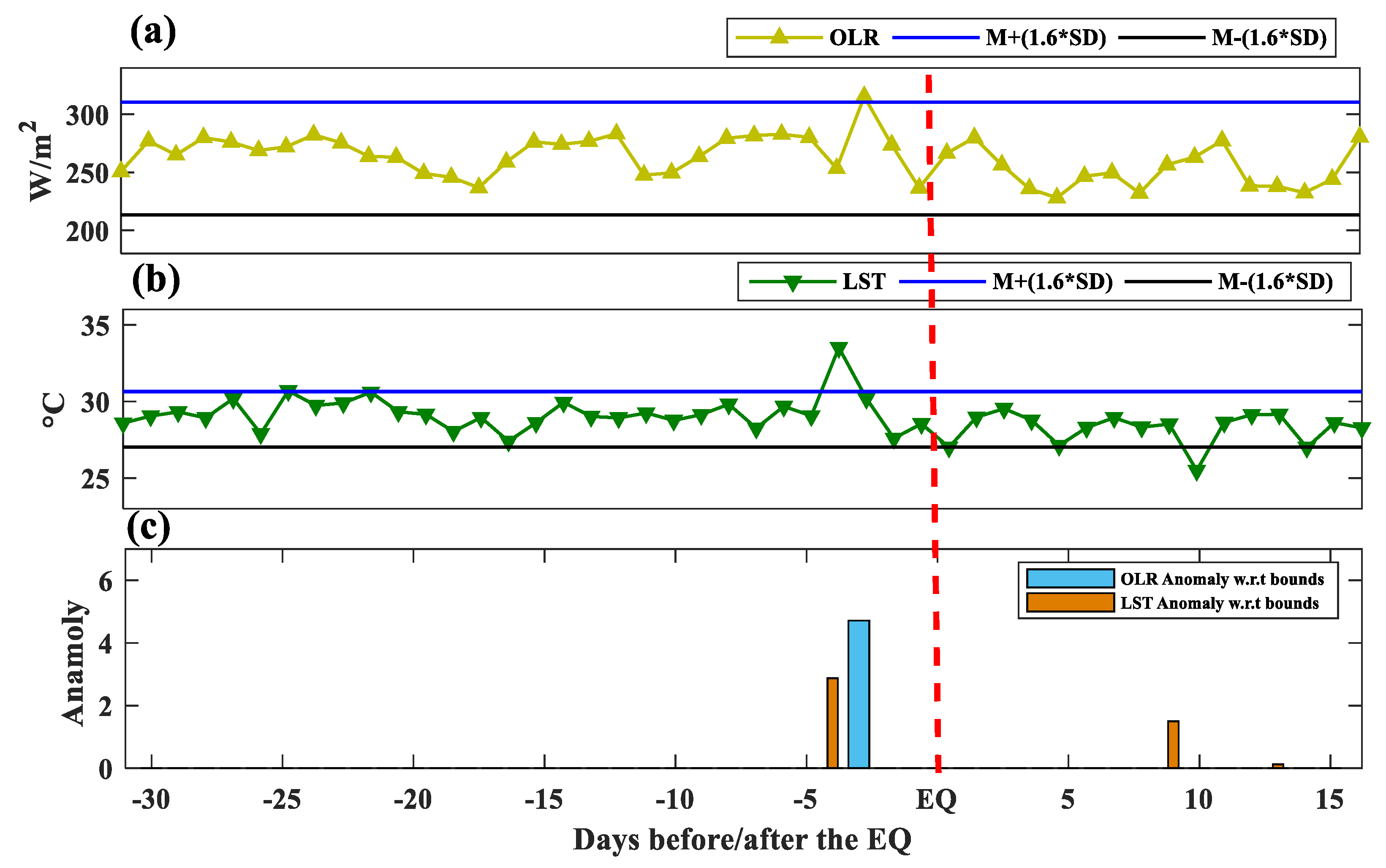
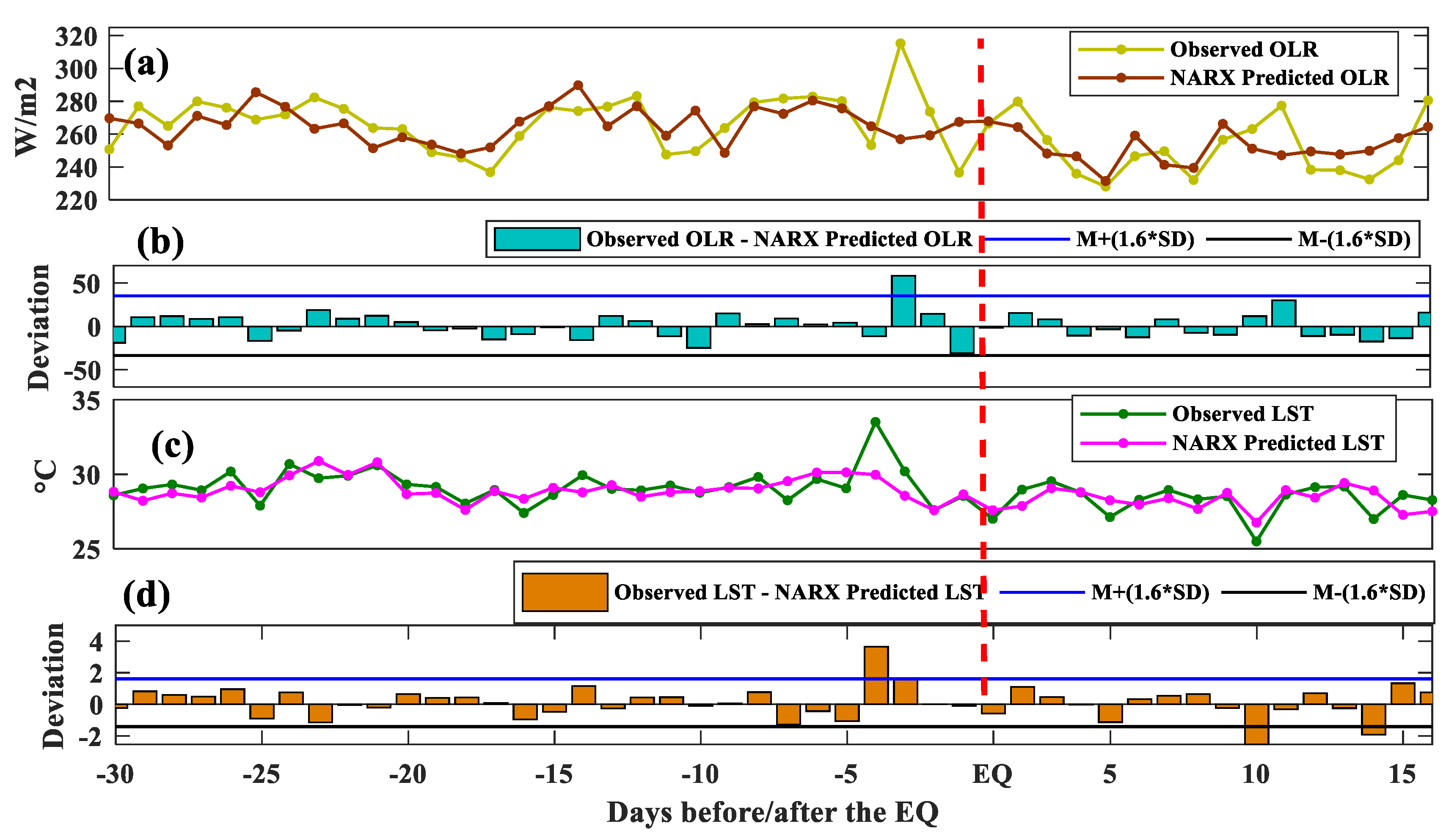
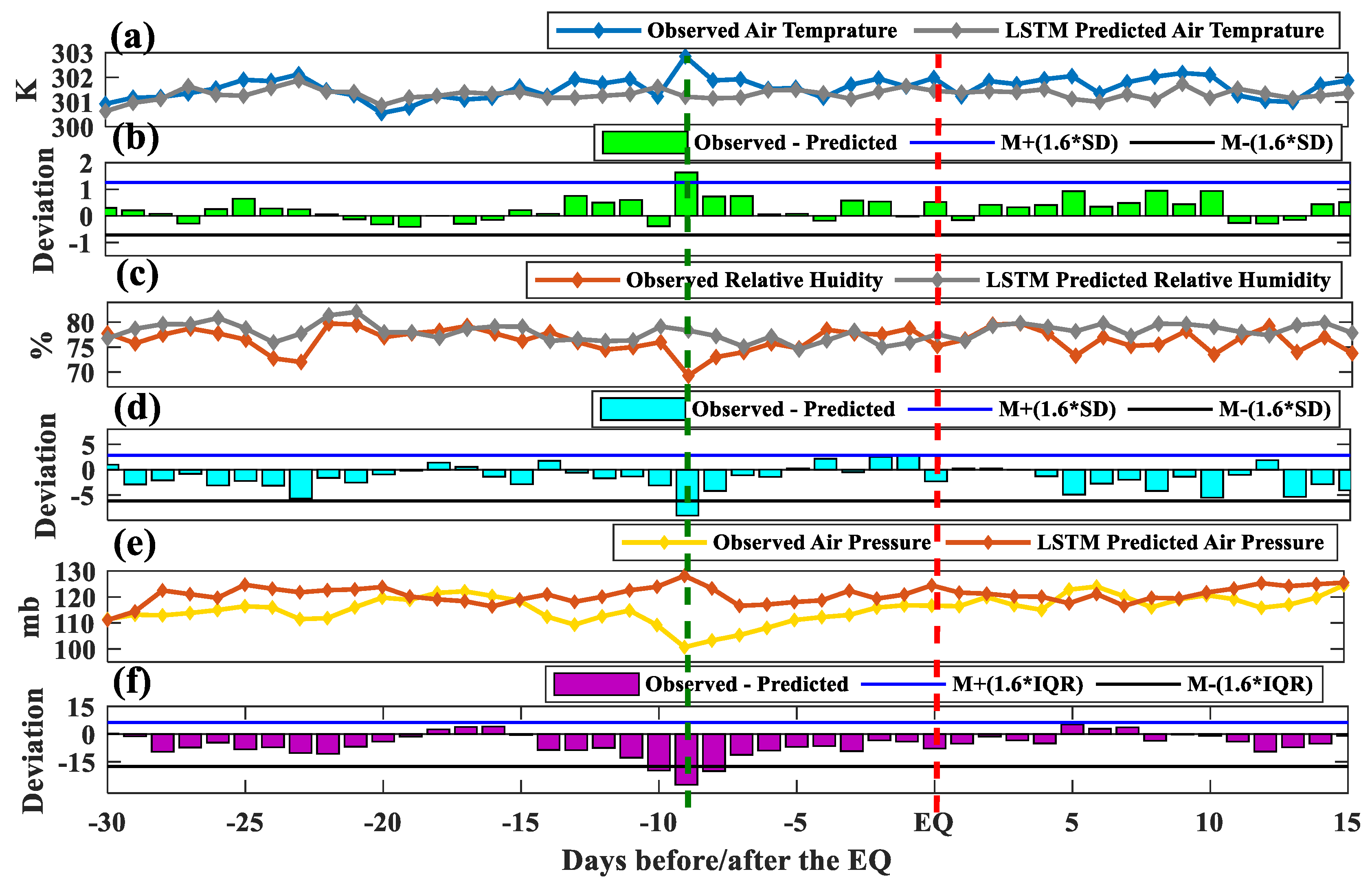
- The LST, AT, RH, AP, and OLR show an unusual variation beyond the defined bounds in the statistical analysis during the 10-day window prior to the seismic event.
- (2)
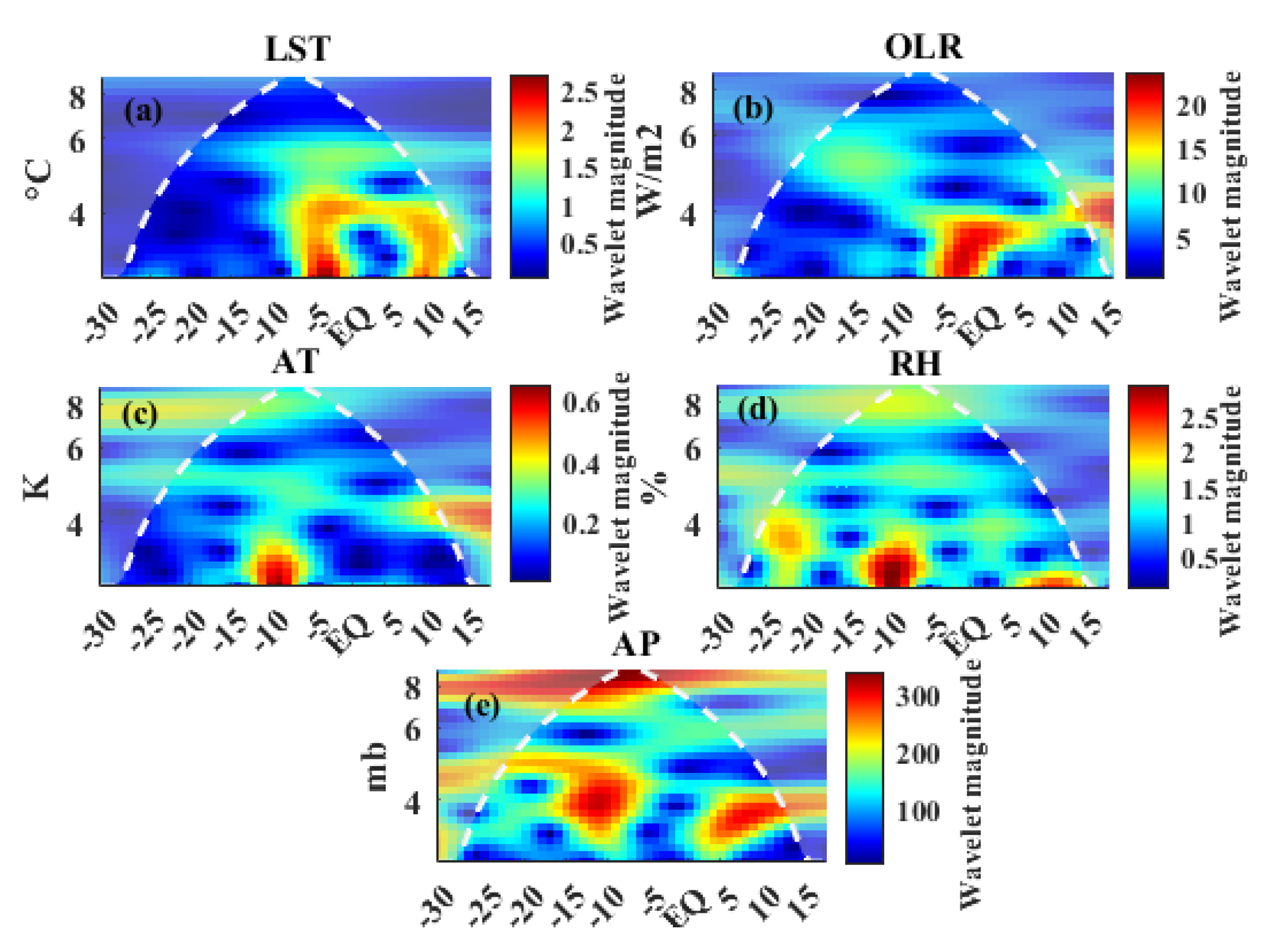
- The anomalous behavior of all the atmospheric parameters is confirmed in wavelet transformations by the local maxima approximation from the time series data within 5–10 days before the EQ.
- (3)
- While using NARX and LSTM algorithms, the maximum of AT, RH, and AP deviation between the observed and predicted values was 5–10 days before the main shock. Nevertheless, for LST and OLR, anomalies occurred within the 5 days before the EQ main shock.
Author Contributions
Funding
Institutional Review Board Statement
Informed Consent Statement
Data Availability Statement
Acknowledgments
Conflicts of Interest
References
- Liu, J.Y.; Chuo, Y.J.; Shan, S.J.; Tsai, Y.B.; Chen, Y.I.; Pulinets, S.; Yu, S.B. Pre-earthquake ionospheric anomalies registered by continuous GPS TEC measurements. Ann. Geophys. 2004, 22, 1585–1593. [Google Scholar] [CrossRef]
- Pulinets, S.; Dunajecka, M. Specific variations of air temperature and relative humidity around the time of Michoacan earthquake M8.1 Sept. 19, 1985 as a possible indicator of interaction between tectonic plates. Tectonophysics 2007, 431, 221–230. [Google Scholar] [CrossRef]
- Kuo, C.L.; Lee, L.C.; Huba, J.D. An improved coupling model for the lithosphere-atmosphere-ionosphere system. J. Geophys. Res. Space Phys. 2014, 119, 3189–3205. [Google Scholar] [CrossRef]
- Daneshvar, M.R.M.; Freund, F.T. Remote Sensing of Atmospheric and Ionospheric Signals Prior to the Mw 8.3 Illapel Earthquake, Chile 2015. Pure Appl. Geophys. 2016, 174, 11–45. [Google Scholar] [CrossRef]
- Freeshah, M.; Zhang, X.; Şentürk, E.; Adil, M.A.; Mousa, B.G.; Tariq, A.; Ren, X.; Refaat, M. Analysis of Atmospheric and Ionospheric Variations Due to Impacts of Super Typhoon Mangkhut (1822) in the Northwest Pacific Ocean. Remote Sens. 2021, 13, 661. [Google Scholar] [CrossRef]
- Hafeez, A.; Ehsan, M.; Abbas, A.; Shah, M.; Shahzad, R. Machine learning-based thermal anomalies detection from MODIS LST associated with the Mw 7.7 Awaran, Pakistan earthquake. Nat. Hazards 2022, 111, 2097–2115. [Google Scholar] [CrossRef]
- Hafeez, A.; Shah, M.; Ehsan, M.; Jamjareegulgarn, P.; Ahmed, J.; Tariq, M.A.; Iqbal, S.; Naqvi, N.A. Possible Atmosphere and Ionospheric Anomalies of the 2019 Pakistan Earthquake Using Statistical and Machine Learning Procedures on MODIS LST, GPS TEC, and GIM TEC. IEEE J. Sel. Top. Appl. Earth Obs. Remote Sens. 2021, 14, 11126–11133. [Google Scholar] [CrossRef]
- Xu, X.; Chen, S.; Yu, Y.; Zhang, S. Atmospheric Anomaly Analysis Related to Ms > 6.0 Earthquakes in China during 2020–2021. Remote Sens. 2021, 13, 4052. [Google Scholar] [CrossRef]
- Shah, M.; Jin, S. Pre-seismic ionospheric anomalies of the 2013 Mw = 7.7 Pakistan earthquake from GPS and COSMIC observations. Geodesy Geodyn. 2018, 9, 378–387. [Google Scholar] [CrossRef]
- Wei, L.; Li, J.; Liu, L.; Huang, L.; Zheng, D.; Tian, X.; Huang, L.; Zhou, L.; Ren, C.; He, H. Lithosphere Ionosphere Coupling Associated with Seismic Swarm in the Balkan Peninsula from ROB-TEC and GPS. Remote Sens. 2022, 14, 4759. [Google Scholar] [CrossRef]
- Geller, R.J. Earthquake prediction: A critical review. Geophys. J. Int. 1997, 131, 425–450. [Google Scholar] [CrossRef]
- Pulinets, S.; Ouzounov, D. Lithosphere–Atmosphere–Ionosphere Coupling (LAIC) model—An unified concept for earthquake precursors validation. J. Southeast Asian Earth Sci. 2011, 41, 371–382. [Google Scholar] [CrossRef]
- Kojima, H.; Yoshino, C.; Nemoto, K.; Hattori, K.; Konishi, T.; Furuya, R. Multi-channel singular spectrum analysis of underground Rn concentration at Asahi station, Boso Peninsula, Japan: Preliminary report on relation between the variation of underground Rn flux and the local seismic activity. J. Atmospheric Electr. 2020, 39, 46–51. [Google Scholar] [CrossRef]
- Deb, A.; Gazi, M.; Barman, C. Anomalous soil radon fluctuations—Signal of earthquakes in Nepal and eastern India regions. J. Earth Syst. Sci. 2016, 125, 1657–1665. [Google Scholar] [CrossRef]
- D’Alessandro, A.; Scudero, S.; Siino, M.; Alessandro, G.; Mineo, R. Long-Term Monitoring and Characterization of Soil Radon Emission in a Seismically Active Area. Geochem. Geophys. Geosystems 2020, 21, e2020GC009061. [Google Scholar] [CrossRef]
- Salikhov, N.; Shepetov, A.; Pak, G.; Nurakynov, S.; Ryabov, V.; Saduyev, N.; Sadykov, T.; Zhantayev, Z.; Zhukov, V. Monitoring of Gamma Radiation Prior to Earthquakes in a Study of Lithosphere-Atmosphere-Ionosphere Coupling in Northern Tien Shan. Atmosphere 2022, 13, 1667. [Google Scholar] [CrossRef]
- Adil, M.A.; Şentürk, E.; Pulinets, S.A.; Amory-Mazaudier, C. A Lithosphere–Atmosphere–Ionosphere Coupling Phenomenon Observed Before M 7.7 Jamaica Earthquake. Pure Appl. Geophys. 2021, 178, 3869–3886. [Google Scholar] [CrossRef]
- Freund, F.; Ouillon, G.; Scoville, J.; Sornette, D. Earthquake precursors in the light of peroxy defects theory: Critical review of systematic observations. Eur. Phys. J. Speéc. Top. 2021, 230, 7–46. [Google Scholar] [CrossRef]
- Jiao, Z.; Shan, X. Pre-Seismic Temporal Integrated Anomalies from Multiparametric Remote Sensing Data. Remote Sens. 2022, 14, 2343. [Google Scholar] [CrossRef]
- Dobrovolsky, I.P.; Zubkov, S.I.; Miachkin, V.I. Estimation of the size of earthquake preparation zones. Pure Appl. Geophys. 1979, 117, 1025–1044. [Google Scholar] [CrossRef]
- U.S. Geological Survey, 2020, Earthquake Lists, Maps, and Statistics. Available online: https://www.usgs.gov/natural-hazards/earthquake-hazards/lists-maps-and-statistics (accessed on 18 June 2022).
- Ouzounov, D.; Freund, F. Mid-infrared emission prior to strong earthquakes analyzed by remote sensing data. Adv. Space Res. 2004, 33, 268–273. [Google Scholar] [CrossRef]
- Chen, S.; Liu, P.; Feng, T.; Wang, D.; Jiao, Z.; Chen, L.; Xu, Z.; Zhang, G. Exploring Changes in Land Surface Temperature Possibly Associated with Earthquake: Case of the April 2015 Nepal Mw 7.9 Earthquake. Entropy 2020, 22, 377. [Google Scholar] [CrossRef]
- Monteiro, L.d.S.; de Oliveira-Júnior, J.F.; Ghaffar, B.; Tariq, A.; Qin, S.; Mumtaz, F.; Filho, W.L.F.C.; Shah, M.; Jardim, A.M.D.R.F.; da Silva, M.V.; et al. Rainfall in the Urban Area and Its Impact on Climatology and Population Growth. Atmosphere 2022, 13, 1610. [Google Scholar] [CrossRef]
- Daily Climate Composites: NOAA Physical Sciences Laboratory, Boulder, Colorado, USA. Available online: https://psl.noaa.gov/data/composites/day/ (accessed on 18 October 2022).
- Shah, M.; Abbas, A.; Adil, M.A.; Ashraf, U.; de Oliveira-Júnior, J.F.; Tariq, M.A.; Ahmed, J.; Ehsan, M.; Ali, A. Possible seismo-ionospheric anomalies associated with M > 5.0 earthquakes during 2000–2020 from GNSS TEC. Adv. Space Res. 2022, 70, 179–187. [Google Scholar] [CrossRef]
- de Oliveira-Júnior, J.F.; Shah, M.; Abbas, A.; Filho, W.L.F.C.; Junior, C.A.D.S.; Santiago, D.D.B.; Teodoro, P.E.; Mendes, D.; de Souza, A.; Aviv-Sharon, E.; et al. Spatiotemporal Analysis of Fire Foci and Environmental Degradation in the Biomes of Northeastern Brazil. Sustainability 2022, 14, 6935. [Google Scholar] [CrossRef]
- Tariq, M.A.; Shah, M.; Li, Z.; Wang, N.; Iqbal, T.; Liu, L. Lithosphere ionosphere coupling associated with three earthquakes in Pakistan from GPS and GIM TEC. J. Geodyn. 2021, 147, 101860. [Google Scholar] [CrossRef]
- Mehdi, S.; Shah, M.; Naqvi, N.A. Lithosphere atmosphere ionosphere coupling associated with the 2019 Mw 7.1 California earthquake using GNSS and multiple satellites. Environ. Monit. Assess. 2021, 193, 501. [Google Scholar] [CrossRef]
- Adil, M.A.; Abbas, A.; Ehsan, M.; Shah, M.; Naqvi, N.A.; Alie, A. Investigation of ionospheric and atmospheric anomalies associated with three Mw > 6.5 EQs in New Zealand. J. Geodyn. 2021, 145, 101841. [Google Scholar] [CrossRef]
- Pulinets, S.A.; Ouzounov, D.; Karelin, A.V.; Davidenko, D. Physical bases of the generation of short-term earthquake precursors: A complex model of ionization-induced geophysical processes in the lithosphere-atmosphere-ionosphere-magnetosphere system. Geomagn. Aeron. 2015, 55, 521–538. [Google Scholar] [CrossRef]
- Shahzad, R.; Shah, M.; Ahmed, A. Comparison of VTEC from GPS and IRI-2007, IRI-2012 and IRI-2016 over Sukkur Pakistan. Astrophys. Space Sci. 2021, 366, 42. [Google Scholar] [CrossRef]
- Shah, M.; Aibar, A.C.; Tariq, M.A.; Ahmed, J.; Ahmed, A. Possible ionosphere and atmosphere precursory analysis related to Mw > 6.0 earthquakes in Japan. Remote Sens. Environ. 2019, 239, 111620. [Google Scholar] [CrossRef]
- Adil, M.A.; Şentürk, E.; Shah, M.; Naqvi, N.A.; Saqib, M.; Abbasi, A.R. Atmospheric and ionospheric disturbances associated with the M > 6 earthquakes in the East Asian sector: A case study of two consecutive earthquakes in Taiwan. J. Southeast Asian Earth Sci. 2021, 220, 104918. [Google Scholar] [CrossRef]
- Shah, M.; Qureshi, R.U.; Khan, N.G.; Ehsan, M.; Yan, J. Artificial Neural Network based thermal anomalies associated with earthquakes in Pakistan from MODIS LST. J. Atmospheric Solar-Terrestrial Phys. 2021, 215, 105568. [Google Scholar] [CrossRef]
- Shah, M.; Ahmed, A.; Ehsan, M.; Khan, M.; Tariq, M.A.; Calabia, A.; Rahman, Z.U. Total electron content anomalies associated with earthquakes occurred during 1998–2019. Acta Astronaut. 2020, 175, 268–276. [Google Scholar] [CrossRef]
- Shah, M.; Inyurt, S.; Ehsan, M.; Ahmed, A.; Shakir, M.; Ullah, S.; Iqbal, M.S. Seismo ionospheric anomalies in Turkey associated with M ≥ 6.0 earthquakes detected by GPS stations and GIM TEC. Adv. Space Res. 2020, 65, 2540–2550. [Google Scholar] [CrossRef]
- Kiyani, A.; Shah, M.; Ahmed, A.; Shah, H.H.; Hameed, S.; Adil, M.A.; Naqvi, N.A. Seismo ionospheric anomalies possibly associated with the 2018 M 8.2 Fiji earthquake detected with GNSS TEC. J. Geodyn. 2020, 140, 101782. [Google Scholar] [CrossRef]
- Pulinets, S.A.; Ouzounov, D.; Ciraolo, L.; Singh, R.; Cervone, G.; Leyva, A.; Dunajecka, M.; Karelin, A.V.; Boyarchuk, K.A.; Kotsarenko, A. Thermal, atmospheric and ionospheric anomalies around the time of the Colima M7.8 earthquake of 21 January 2003. Ann. Geophys. 2006, 24, 835–849. [Google Scholar] [CrossRef]
- Pavlidou, E.; van der Meijde, M.; van der Werff, H.; Hecker, C. Time Series Analysis of Land Surface Temperatures in 20 Earthquake Cases Worldwide. Remote Sens. 2018, 11, 61. [Google Scholar] [CrossRef]
- Liu, J.; Hagan, D.F.T.; Holmes, T.R.; Liu, Y. An Analysis of Spatio-Temporal Relationship between Satellite-Based Land Surface Temperature and Station-Based Near-Surface Air Temperature over Brazil. Remote Sens. 2022, 14, 4420. [Google Scholar] [CrossRef]
- Abbasi, A.R.; Shah, M.; Ahmed, A.; Naqvi, N.A. Possible ionospheric anomalies associated with the 2009 Mw 6.4 Taiwan earthquake from DEMETER and GNSS TEC. Acta Geod. et Geophys. 2020, 56, 77–91. [Google Scholar] [CrossRef]
- Shah, M.; Tariq, M.A.; Naqvi, N.A. Atmospheric anomalies associated with Mw>6.0 earthquakes in Pakistan and Iran during 2010–2017. J. Atmos. Solar-Terr. Phys. 2019, 191, 105056. [Google Scholar] [CrossRef]
- Ouzounov, D.; Liu, D.; Chunli, K.; Cervone, G.; Kafatos, M.; Taylor, P. Outgoing long wave radiation variability from IR satellite data prior to major earthquakes. Tectonophysics 2007, 431, 211–220. [Google Scholar] [CrossRef]
- Boyarchuk, K.; Lomonosov, A.; Pulinets, S.A.; Hegai, V.V. Variability of the Earth’s Atmospheric Electric Field and Ion-Aerosols Kinetics in the Troposphere. Stud. Geophys. et Geod. 1998, 42, 197–210. [Google Scholar] [CrossRef]
- Zhang, Z.; Luo, C.; Zhao, Z. Application of probabilistic method in maximum tsunami height prediction considering stochastic seabed topography. Nat. Hazards 2020, 104, 2511–2530. [Google Scholar] [CrossRef]
- Alam, Z.; Sun, L.; Zhang, C.; Samali, B. Influence of seismic orientation on the statistical distribution of nonlinear seismic response of the stiffness-eccentric structure. Structures 2022, 39, 387–404. [Google Scholar] [CrossRef]
- Xu, J.; Zhou, L.; Li, Y.; Ding, J.; Wang, S.; Cheng, W.-C. Experimental Study on Uniaxial Compression Behavior of Fissured Loess Before and After Vibration. Int. J. Geomech. 2022, 22, 04021277. [Google Scholar] [CrossRef]
- Yue, Z.; Zhou, W.; Li, T. Impact of the Indian Ocean Dipole on Evolution of the Subsequent ENSO: Relative Roles of Dynamic and Thermodynamic Processes. J. Clim. 2021, 34, 3591–3607. [Google Scholar] [CrossRef]
- Zhang, K.; Ali, A.; Antonarakis, A.; Moghaddam, M.; Saatchi, S.; Tabatabaeenejad, A.; Chen, R.; Jaruwatanadilok, S.; Cuenca, R.; Crow, W.T.; et al. The Sensitivity of North American Terrestrial Carbon Fluxes to Spatial and Temporal Variation in Soil Moisture: An Analysis Using Radar-Derived Estimates of Root-Zone Soil Moisture. J. Geophys. Res. Biogeosciences 2019, 124, 3208–3231. [Google Scholar] [CrossRef]
- Wang, S.; Zhang, K.; Chao, L.; Li, D.; Tian, X.; Bao, H.; Chen, G.; Xia, Y. Exploring the utility of radar and satellite-sensed precipitation and their dynamic bias correction for integrated prediction of flood and landslide hazards. J. Hydrol. 2021, 603, 126964. [Google Scholar] [CrossRef]
- Mao, Y.; Sun, R.; Wang, J.; Cheng, Q.; Kiong, L.C.; Ochieng, W.Y. New time-differenced carrier phase approach to GNSS/INS integration. GPS Solut. 2022, 26, 122. [Google Scholar] [CrossRef]
- Li, Z.-J.; Zhang, K. Comparison of Three GIS-Based Hydrological Models. J. Hydrol. Eng. 2008, 13, 364–370. [Google Scholar] [CrossRef]
- Xie, W.; Li, X.; Jian, W.; Yang, Y.; Liu, H.; Robledo, L.; Nie, W. A Novel Hybrid Method for Landslide Susceptibility Mapping-Based GeoDetector and Machine Learning Cluster: A Case of Xiaojin County, China. ISPRS Int. J. Geo-Inf. 2021, 10, 93. [Google Scholar] [CrossRef]
- Xie, W.; Nie, W.; Saffari, P.; Robledo, L.F.; Descote, P.-Y.; Jian, W. Landslide hazard assessment based on Bayesian optimization–support vector machine in Nanping City, China. Nat. Hazards 2021, 109, 931–948. [Google Scholar] [CrossRef]
- Wang, G.; Zhao, B.; Wu, B.; Wang, M.; Liu, W.; Zhou, H.; Zhang, C.; Wang, Y.; Han, Y. Research on the Macro-Mesoscopic Response Mechanism of Multisphere Approximated Heteromorphic Tailing Particles. Lithosphere 2022, 2022, 1977890. [Google Scholar] [CrossRef]
- Wang, G.; Zhao, B.; Wu, B.; Zhang, C.; Liu, W. Intelligent prediction of slope stability based on visual exploratory data analysis of 77 in situ cases. Int. J. Min. Sci. Technol. 2022. [Google Scholar] [CrossRef]
- Zhu, Z.; Wu, Y.; Liang, Z. Mining-Induced Stress and Ground Pressure Behavior Characteristics in Mining a Thick Coal Seam With Hard Roofs. Front. Earth Sci. 2022, 10, 843191. [Google Scholar] [CrossRef]
- Wu, X.; Liu, Z.; Yin, L.; Zheng, W.; Song, L.; Tian, J.; Yang, B.; Liu, S. A Haze Prediction Model in Chengdu Based on LSTM. Atmosphere 2021, 12, 1479. [Google Scholar] [CrossRef]
- Yin, L.; Wang, L.; Huang, W.; Liu, S.; Yang, B.; Zheng, W. Spatiotemporal Analysis of Haze in Beijing Based on the Multi-Convolution Model. Atmosphere 2021, 12, 1408. [Google Scholar] [CrossRef]
- Yin, L.; Wang, L.; Zheng, W.; Ge, L.; Tian, J.; Liu, Y.; Yang, B.; Liu, S. Evaluation of Empirical Atmospheric Models Using Swarm-C Satellite Data. Atmosphere 2022, 13, 294. [Google Scholar] [CrossRef]
- Zhang, X.; Ma, F.; Yin, S.; Wallace, C.D.; Soltanian, M.R.; Dai, Z.; Ritzi, R.W.; Ma, Z.; Zhan, C.; Lü, X. Application of upscaling methods for fluid flow and mass transport in multi-scale heterogeneous media: A critical review. Appl. Energy 2021, 303, 117603. [Google Scholar] [CrossRef]
- Huang, S.; Liu, C. A computational framework for fluid–structure interaction with applications on stability evaluation of breakwater under combined tsunami–earthquake activity. Comput. Civ. Infrastruct. Eng. 2022, 1–28. [Google Scholar] [CrossRef]
- Li, J.; Cheng, F.; Lin, G.; Wu, C. Improved Hybrid Method for the Generation of Ground Motions Compatible with the Multi-Damping Design Spectra. J. Earthq. Eng. 2022, 2, 20–26. [Google Scholar] [CrossRef]
- Huang, S.; Lyu, Y.; Sha, H.; Xiu, L. Seismic performance assessment of unsaturated soil slope in different groundwater levels. Landslides 2021, 18, 2813–2833. [Google Scholar] [CrossRef]
- Tian, H.; Qin, Y.; Niu, Z.; Wang, L.; Ge, S. Summer Maize Mapping by Compositing Time Series Sentinel-1A Imagery Based on Crop Growth Cycles. J. Indian Soc. Remote Sens. 2021, 49, 2863–2874. [Google Scholar] [CrossRef]
- Tian, H.; Wang, Y.; Chen, T.; Zhang, L.; Qin, Y. Early-Season Mapping of Winter Crops Using Sentinel-2 Optical Imagery. Remote Sens. 2021, 13, 3822. [Google Scholar] [CrossRef]
- Chen, L.; Huang, Y.; Yu, X.; Lu, J.; Jia, W.; Song, J.; Liu, L.; Wang, Y.; Huang, Y.; Xie, J.; et al. Corynoxine Protects Dopaminergic Neurons Through Inducing Autophagy and Diminishing Neuroinflammation in Rotenone-Induced Animal Models of Parkinson’s Disease. Front. Pharmacol. 2021, 12, 642900. [Google Scholar] [CrossRef] [PubMed]
- Zhao, M.; Zhou, Y.; Li, X.; Cheng, W.; Zhou, C.; Ma, T.; Li, M.; Huang, K. Mapping urban dynamics (1992–2018) in Southeast Asia using consistent nighttime light data from DMSP and VIIRS. Remote Sens. Environ. 2020, 248, 111980. [Google Scholar] [CrossRef]
- Zhao, M.; Zhou, Y.; Li, X.; Zhou, C.; Cheng, W.; Li, M.; Huang, K. Building a Series of Consistent Night-Time Light Data (1992–2018) in Southeast Asia by Integrating DMSP-OLS and NPP-VIIRS. IEEE Trans. Geosci. Remote Sens. 2019, 58, 1843–1856. [Google Scholar] [CrossRef]
- Qu, J.; Feng, Y.; Xu, G.; Zhang, M.; Zhu, Y.; Zhou, S. Design and thermodynamics analysis of marine dual fuel low speed engine with methane reforming integrated high pressure exhaust gas recirculation system. Fuel 2022, 319, 123747. [Google Scholar] [CrossRef]
- Yang, J.; Fu, L.-Y.; Zhang, Y.; Han, T. Temperature- and Pressure-Dependent Pore Microstructures Using Static and Dynamic Moduli and Their Correlation. Rock Mech. Rock Eng. 2022, 55, 4073–4092. [Google Scholar] [CrossRef]
- Cheng, Y.; Fu, L.-Y. Nonlinear seismic inversion by physics-informed Caianiello convolutional neural networks for overpressure prediction of source rocks in the offshore Xihu depression, East China. J. Pet. Sci. Eng. 2022, 215, 110654. [Google Scholar] [CrossRef]
- Zhao, F.; Song, L.; Peng, Z.; Yang, J.; Luan, G.; Chu, C.; Ding, J.; Feng, S.; Jing, Y.; Xie, Z. Night-Time Light Remote Sensing Mapping: Construction and Analysis of Ethnic Minority Development Index. Remote Sens. 2021, 13, 2129. [Google Scholar] [CrossRef]
- Zhao, F.; Zhang, S.; Du, Q.; Ding, J.; Luan, G.; Xie, Z. Assessment of the sustainable development of rural minority settlements based on multidimensional data and geographical detector method: A case study in Dehong, China. Socio-Economic Plan. Sci. 2021, 78, 101066. [Google Scholar] [CrossRef]
- Shah, M.; Ehsan, M.; Abbas, A.; Ahmed, A.; Jamjareegulgarn, P. Possible Thermal Anomalies Associated With Global Terrestrial Earthquakes During 2000–2019 Based on MODIS-LST. IEEE Geosci. Remote Sens. Lett. 2021, 19, 1–5. [Google Scholar] [CrossRef]
- Shah, M.; Abbas, A.; Ehsan, M.; Calabia, A.; Adhikari, B.; Tariq, M.A.; Ahmed, J.; de Oliveira-Junior, J.F.; Yan, J.; Melgarejo-Morales, A.; et al. Ionospheric–Thermospheric Responses in South America to the August 2018 Geomagnetic Storm Based on Multiple Observations. IEEE J. Sel. Top. Appl. Earth Obs. Remote Sens. 2021, 15, 261–269. [Google Scholar] [CrossRef]
- Shah, M.; Tariq, M.A.; Ahmad, J.; Naqvi, N.A.; Jin, S. Seismo ionospheric anomalies before the 2007 M7.7 Chile earthquake from GPS TEC and DEMETER. J. Geodyn. 2019, 127, 42–51. [Google Scholar] [CrossRef]
- Shah, M.; Jin, S. Statistical characteristics of seismo-ionospheric GPS TEC disturbances prior to global Mw≥5.0 earthquakes (1998–2014). J. Geodyn. 2015, 92, 42–49. [Google Scholar] [CrossRef]
- Tariq, M.A.; Shah, M.; Hernández-Pajares, M.; Iqbal, T. Pre-earthquake ionospheric anomalies before three major earthquakes by GPS-TEC and GIM-TEC data during 2015–2017. Adv. Space Res. 2019, 63, 2088–2099. [Google Scholar] [CrossRef]
- Ahmed, J.; Shah, M.; Zafar, W.A.; Amin, M.A.; Iqbal, T. Seismoionospheric anomalies associated with earthquakes from the analysis of the ionosonde data. J. Atmos. Sol.-Terr. Phys. 2018, 179, 450–458. [Google Scholar] [CrossRef]
- Liu, X.; Zhang, Q.; Shah, M.; Hong, Z. Atmospheric-ionospheric disturbances following the April 2015 Calbuco volcano from GPS and OMI observations. Adv. Space Res. 2017, 60, 2836–2846. [Google Scholar] [CrossRef]
- Shah, M.; Khan, M.; Ullah, H.; Ali, S. Thermal Anomalies Prior to The 2015 Gorkha (Nepal) Earthquake From Modis Land Surface Temperature and Outgoing Longwave Radiations. Geodyn. Tectonophys. 2018, 9, 123–138. [Google Scholar] [CrossRef]
- Hussain, A.; Shah, M. Comparison of GPS TEC with IRI models of 2007, 2012, & 2016 over Sukkur, Pakistan. Nat. Appl. Sci. Int. J. (NASIJ) 2020, 1, 1–10. [Google Scholar] [CrossRef]


| Time of Anomaly Observation (Days) | ||||
|---|---|---|---|---|
| Parameter | IQR | Wavelet | NARX | LSTM |
| AT | −9 | −10 and −9 | −9 | −9 |
| RH | −9 | −10 and −9 | −9 | −9 |
| AP | −9 and −8 | −10 to −8 | −9 | −10 to −8 |
| LST | −4 | −4 | −4 | −4 |
| OLR | −3 | −3 | −3 | −3 |
Publisher’s Note: MDPI stays neutral with regard to jurisdictional claims in published maps and institutional affiliations. |
© 2022 by the authors. Licensee MDPI, Basel, Switzerland. This article is an open access article distributed under the terms and conditions of the Creative Commons Attribution (CC BY) license (https://creativecommons.org/licenses/by/4.0/).
Share and Cite
Khan, M.M.; Ghaffar, B.; Shahzad, R.; Khan, M.R.; Shah, M.; Amin, A.H.; Eldin, S.M.; Naqvi, N.A.; Ali, R. Atmospheric Anomalies Associated with the 2021 Mw 7.2 Haiti Earthquake Using Machine Learning from Multiple Satellites. Sustainability 2022, 14, 14782. https://doi.org/10.3390/su142214782
Khan MM, Ghaffar B, Shahzad R, Khan MR, Shah M, Amin AH, Eldin SM, Naqvi NA, Ali R. Atmospheric Anomalies Associated with the 2021 Mw 7.2 Haiti Earthquake Using Machine Learning from Multiple Satellites. Sustainability. 2022; 14(22):14782. https://doi.org/10.3390/su142214782
Chicago/Turabian StyleKhan, Muhammad Muzamil, Bushra Ghaffar, Rasim Shahzad, M. Riaz Khan, Munawar Shah, Ali H. Amin, Sayed M. Eldin, Najam Abbas Naqvi, and Rashid Ali. 2022. "Atmospheric Anomalies Associated with the 2021 Mw 7.2 Haiti Earthquake Using Machine Learning from Multiple Satellites" Sustainability 14, no. 22: 14782. https://doi.org/10.3390/su142214782
APA StyleKhan, M. M., Ghaffar, B., Shahzad, R., Khan, M. R., Shah, M., Amin, A. H., Eldin, S. M., Naqvi, N. A., & Ali, R. (2022). Atmospheric Anomalies Associated with the 2021 Mw 7.2 Haiti Earthquake Using Machine Learning from Multiple Satellites. Sustainability, 14(22), 14782. https://doi.org/10.3390/su142214782