Association between Land Surface Temperature and Green Volume in Bochum, Germany

Abstract

Average temperatures continue to rise throughout the world due to climate change and, thus, also in Europe, often occurring as heat waves. The negative effects of climate change-related heat waves can be observed, especially in urban areas where land sealing is the greatest and so is population density. Past studies have indicated that green volume can provide climate improvement by balancing humidity and regulating temperature. This study aims to estimate the distribution of surface heat islands and green volume and test the relationship between these variables in a case study of Bochum, Germany. A method to develop a temporally longitudinal 30-m Landsat 8-based land surface temperature (LST) analysis and 30-m LiDAR-based green volume dataset are presented, and their relationship is tested using Pearson’s correlation (n = 148,204). The results show that heat islands are moderately negatively correlated with green volume (r = −0.482; p < 0.05), LST can vary as much as 28 degrees °C between heat islands and densely vegetated areas, and the distribution is heterogeneous across Bochum.

1. Introduction

Urban areas generally have higher surface and air temperatures than the surrounding areas [1]. However, temperature differences also occur within urban areas. Increased thermal stress can result from, among other things, building density, the degree of sealing, and a lack of green spaces in urban areas. Therefore, thermal stress directly impacts the inhabitants’ well-being and quality of life [1]. Furthermore, the intensification of extreme weather events such as heat waves or a general increase in global temperature predicted in connection with climate change intensify these existing burdens [2]. What is striking here is the speed of this development, which is occurring quickly compared to climate changes in the history of the Earth [2]. The reason for this development is the increased release of greenhouse gases such as carbon dioxide. Although efforts to reduce greenhouse gases and, thus, stop global warming and its consequences have intensified, especially within the last decade, these developments can no longer be stopped or reversed [2]. Therefore, strategies must be developed to slow down the described process and to be able to adequately counter the consequences of climate change in cities and metropolitan areas [2].

The negative effects of climate change can be observed, especially in urban areas [3]. On the one hand, due to the increased population density in cities, there is a higher number of vulnerable groups, which can be particularly affected by negative climatic impacts due to their physical or mental constitution. Vulnerable population groups in this context are people over 65 years of age, people without access to air-conditioned indoor spaces, and people with a weakened cardiovascular system [2]. Heat waves are also a health risk for young children due to their unstable thermoregulation [4]. On the other hand, the framework conditions of urban space favor or intensify the climatic developments and effects of climate change [3]. The interaction of correspondingly disadvantageous urban structures, such as a high degree of sealing or a low number of green spaces on the one hand, and the effects of climate change, such as the increase in the annual mean temperature or the increased occurrence of heat waves on the other, can increase heat stress. This can have a negative impact on both the building fabric and the health of the population, for example, in the form of urban heat islands, where temperatures contrast between city and surrounding area [5]) or UHI [3]. With an increase in the global average temperature, a further increase in air temperature in German cities is also to be expected, with an increase or intensification of heat waves [2].

In this context, the connection between UHIs and soil sealing is striking. Soils with vegetation cover have a cooling effect on their surroundings [6]. Urban green spaces are, therefore, suitable for reducing or even preventing UHIs. Urban greenery has different effects on space, depending on its type and configuration. Medium-to-tall vegetation layers, such as trees, primarily produce oxygen [7]. They also bind air pollutants, provide shading and evaporation, and thus positively affect the urban climate (defined as a microclimate formed by cities and metropolitan areas [8]). Low vegetation layers such as meadows and lawns play a crucial role in cold air formation and fresh air exchange. The impact of green spaces on urban climates depends on their size, spatial distribution, and volume [7]. In this context, the increasing size of a green space correlates with its positive effect on the urban climate. This means that, with an increase in green volume, the cooling effect also increases, and the air temperature can be lowered [7]. However, even smaller green spaces that are appropriately spatially distributed have direct cooling effects and positively impact the urban climate despite their local limitations. The so-called green volume (GV)is the “above-ground volume of all plants within a defined surface area” [9] and thus a meaningful indicator in connection with UHIs [7].

Sealed urban surfaces, on the other hand, have heat-absorbing properties. In particular, dark ground surfaces such as asphalt have a low albedo. Albedo “is a measure of […] the reflectivity of different surfaces” [6]. “The albedo can take values between 0 and 1, where the smaller the value the more energy absorbed and the larger the value the more energy reflected“ [10] and can reach temperatures of 50 °C above the actual air temperature. In addition, dark surfaces can absorb more radiation on average than light or natural surfaces such as meadows and forests, which reflect more incoming shortwave radiation and thus absorb less heat energy [10,11]. To compound the albedo effect, sealed surfaces are also usually impermeable to water, and thus, precipitation cannot develop its cooling effect there through soil–water retention and evapotranspiration [6].

1.1. The Formation and Properties of Urban Heat Islands

Urban regions and cities have a characteristic local or urban climate [12]. The World Meteorological Organization (WMO) describes the urban climate as a “local climate altered by building development and emissions compared to the surrounding area” [13]. Thus, the urban climate has been altered by anthropogenic influences and is of particular importance because of a high local population density and the associated high energy consumption [14]. The UHI is a typical feature and best-known urban climate effect. This can be characterized by the difference in air and surface temperatures between the warmer city and the cooler surrounding area [15].

UHIs are subject to diurnal and seasonal fluctuations and depend on prevailing weather conditions [15]. The air temperature difference can reach its maximum on cloudless and windless nights, where it can be “up to 10 Kelvin” (K) in agglomeration areas [16] and also correlates positively with city size [12]. The air temperature in urban areas is influenced by various parameters and depends on, among other things, the prevailing building geometries, the radiative properties of the surfaces, the thermal properties of the buildings, and manmade heat releases such as those caused by industry and traffic [12] (Figure 1).

The name “heat island” is due to the island-like appearance of excessive heating in a colder environment [17]. However, this term is criticized as inaccurate; instead, the term heat archipelago may be more appropriate, since an urban area is not homogeneously overheated but can have several heterogeneously distributed heat centers. The UHI is usually not understood as a single bubble in the atmosphere [18] but rather as several horizontal layers distributed in relation to sealed, dark-colored, or built-up urban surfaces [19]. These horizontal UHI layers include the surface heat island (SHI), vertical heat islands on building facades, the urban barrier heat island that “[…] extends between ground surface and mean roof height. […]. [It] is only partially congruent with the built-up surface.” [18]), and the urban boundary heat island “[…] is formed […] by turbulent heat transport from the bottom to the top, […] and can […] be more than 1000 m thick […].” [18].

Heat island formation is amplified by the high degree of sealing and dense urban development that cannot be sufficiently compensated for by the lack of GV and surface water areas with corresponding cooling capacities [20]. Heat stress in larger cities is, therefore, already considered problematic today and is expected to worsen due to the projected increase in annual mean global temperatures and urban population growth [21]. This is particularly critical in the German state of North-Rhine Westphalia (NRW), where five million urban inhabitants are already affected by adverse thermal situations as of 2018 [8].

The present work deals with the SHI, which is of particular relevance for humans, their quality of life, and health, as it is located at the base of the troposphere where humans live [19]. The SHI depends on the surface temperature and thus can also be detected via satellite data. A SHI occurs when the urban surface temperature is higher than the surrounding surfaces. It is dependent on the building structure and most pronounced during the day [18]. Satellite images and aircraft measurements have established a relationship between recorded surface temperatures and the normalized difference vegetation index (NDVI) as a proxy for urban structures in Berlin and other German cities [22]. In this context, the surface temperature has been found to correlate positively with the percentage of sealed surfaces. Building structures affect SHIs [22], because asphalt and concrete absorb a large part of the incident shortwave radiation due to their low reflectivity and low albedo. The absorbed radiation is stored and released into the ambient air as longwave radiation or latent heat. Buildings and streets are, therefore, a significant contributor to increasing heat loads in cities [23]. In addition, building height and arrangement also influence the temperature; for example, shading in narrow building canyons can cause delayed warming of the street space. At the same time, however, the constriction caused by dense building development can also lead to a reduction in nighttime cooling [24].

1.2. Green Spaces, Green Area, and Green Volume

Green spaces are the most important climate–ecological compensation in urban areas [25] and can offset the effects of SHIs. Physically, evapotranspiration [26] can reduce the land surface temperature (LST) [27] due to heat energy loss during the phase change of water from liquid to gas, thereby reducing the SHI effect. Conversely, LST can increase due to a reduction or absence of vegetation where this process causes a latent heat buildup on urban surfaces [28]. The effect of green areas was estimated to explain 69% of the surface temperature in Rotterdam, NL [29].

In particular, large green spaces such as cemeteries, forests, and parks provide the greatest SHI compensation potential in urban areas [25], because they have a cooling effect on the surrounding buildings and can thus reduce the SHI. During the day, for example, the shady canopy of trees can reduce the latent heat of the area below the canopy. Furthermore, heat storage on the rough surfaces of naturally vegetated soils is significantly less than on asphalt surfaces [30]. In addition, supplementary cooling and increases in humidity occur due to evapotranspiration, as mentioned above. Especially because of the climate change-related increase and intensification of UHIs in Europe, green and open spaces are becoming increasingly important as compensation.

The GV is a suitable environmental indicator and control instrument for climate-adapted urban development. Trees, meadows, shrubs, and other vegetated land cover add up to the GV [31]. The GV concept is similar to units of measure commonly used in building law, for example, the floor area ratio (FAR). The GV was introduced in urban planning to quantify and map the vegetation volume and contains information on an area’s average vegetated volume in m³/m² [32]. GV is a three-dimensional quantity, which necessitates a three-dimensional survey. The derivation of a GV is made possible by using so-called digital terrain models (DTM), which can be derived from laser scanning data such as LiDAR [32]. Thus, GV provides information about the volume of “all plants standing on a green space” [31]. GV is particularly important in urban areas for the natural balance and the well-being of the inhabitants [33]. The greater the volume, the greater the positive impact on the environment [31]. For example, GV improves the climate by balancing the humidity and regulating the temperature [31], which is followed by a decrease in LST [34].

1.3. Problem, Aims, Case Study, and Study Design

Against the background discussed above, it is essential for climate-adapted urban development, harmonizing urban developments with the challenges of climate protection and climate adaptation [3], consider the consequences of climate change and the broad UHI phenomenon. Urban structures that are favorable for SHI layer reduction must be located and their underlying factors understood so that recommendations for action in impacted areas are based on empirical observations of reduced LST [35]. The aim of this study is to identify SHIs in the City of Bochum, Germany, by means of a remote sensing time series of LST analysis and relate this distribution to the metric of GV.

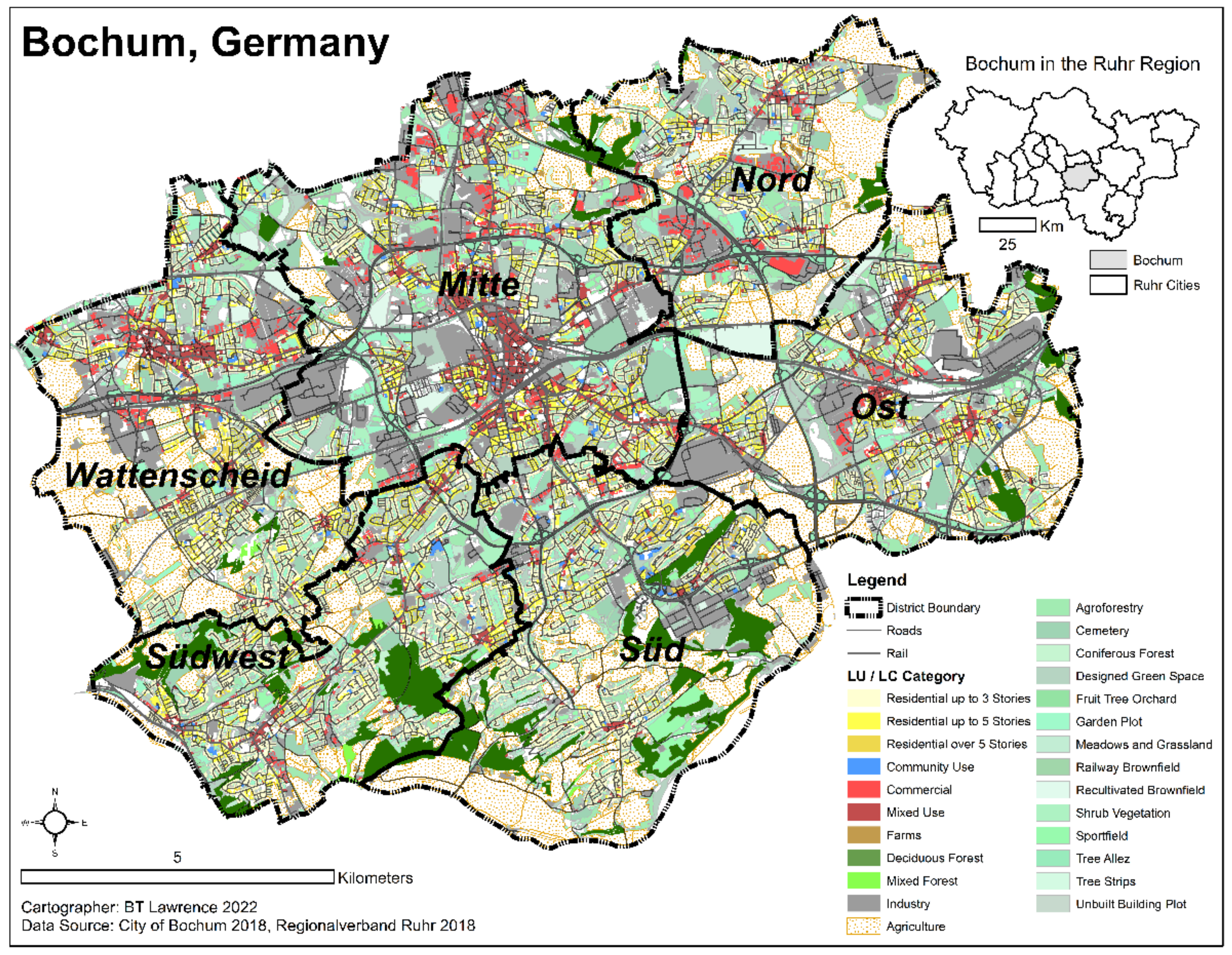
1.3.1. Case Study: Bochum, Germany

The City of Bochum is a good study area to illustrate the impact of urbanization on SHI generation, because it has about 38% sealed surfaces but also generous vegetated land cover [20], a high population density amongst many polycentric urban nodes [36], open access of base data to calculate GV, and, not least, because of the existence of adequate satellite images (Figure 2). Bochum can be assigned to the mid-latitude maritime climate zone [37]. Over the year, temperature ranges are, on average, between 0 and 23 °C [38]. Less frequently, values below −7 °C and above 29 °C are reached. The months from June to September are the typical warm season, where the average daily maximum temperature is above 19 °C. July is the hottest month in Bochum, with an average maximum temperature of 23 °C [38]. As mentioned above, the temperate climate of Central Europe and, thus, also the climate in Bochum is subject to increasingly strong climate change-related fluctuations [39]. Analyzing the annual average temperature for the 1912–2011 period, a slight but steady increase of about 2 Kelvin is observed for Bochum. This temperature increase is due not only to the general climate change, but an estimated 50% of it is caused by Bochum’s urban growth and, thus, the intensification of the urban climate effect [39]. Regarding the need for climate adaptation measures, it is not the described temperature increase that is decisive but rather the total increasing heat load in the inner cities resulting from the shift in European temperature distributions. If heat stress has increased over the last 100 years, it is predicted that the number of days with air temperature above 25 °C will likely double within the next 50 years compared to today [3].

1.3.2. Research Questions and Study Design

The research aims are operationalized into a single concrete research question with four direct sub-questions. Given the homogeneity of the Ruhr region’s spatial–historical development, land cover, and vegetation communities, the work provides insights for other Ruhr cities that have similar configurations. The availability of LiDAR, Landsat 8, and land use/land cover geospatial data Germany-wide means that the analysis methodology presented here will be applicable and repeatable for anywhere in Germany. Thus, this study contributes to understanding the relationship between SHI and GV, specifically in Bochum, but the general methodology is applicable for all of Germany. Unlike past UHI studies in Germany, this study does not rely on proxy indicators, such as the percentage of soil sealing or land use type, to estimate the heat island effects. Instead, it relies on an association between the direct empirical measurements of LST and GV to understand SHI formation. Our questions are:

• How does the green volume affect surface heat islands in Bochum?

  a.

  Does the spatial pattern resemble a heat island or a heat archipelago?

  b.

  What is the correlation between LST and GV?

  c.

  What are the contributions of a vertical structure and type of green space on LST?

  c.

  How do SHI distributions across urban districts relate to human populations?

To assess SHI distribution, the average LST is calculated from Landsat-8 data [40] using the software ENVI (ENVI = Image Processing and Analysis Software for Remote Sensing [41]). The threshold for heat islands is determined based on a literature review, and the heat island pattern in Bochum is subsequently mapped out to address question 1a. A GV dataset is created from LiDAR data, and bivariate correlation is conducted with the LST and GV to address question 1b. To address question 1c, LST and GV are summarized by land cover classification with zonal statistics, and the relationship is depicted with descriptive statistics. The mean LST and GV values are summarized by the city district to address question 1d.

2. Materials and Methods

2.1. Remote Sensing Data to Support LST Anlysis

Remote sensing is used to measure and locate heat islands. Satellite-based remote sensing enables noncontact measurements of bio- and geophysical parameters on the Earth’s surface [42]. Different techniques allow the collection of large-scale and regular data from the atmosphere and the Earth’s surface [15]. Electromagnetic radiation [43], characterized by the electromagnetic spectrum [44]), serves as an information carrier for such measurements [15]. Electromagnetic radiation is absorbed, reflected, or transmitted in different percentages, depending on the properties of a surface [15]. Due to this specific reflection behavior of different surfaces and objects, different information can be obtained [44]. It is precisely this property of a “spectral signature” that modern remote sensing utilizes. As a rule, common remote sensing sensors record image information in the form of pixels. For example, if a pixel size is 30 m, one image pixel represents 30 m × 30 m on the Earth’s surface [45]. The detected radiation or the surface reflections are stored as pixels in the form of so-called digital numbers (DN). The DN report integer values that represent the specific brightness of an image pixel. Using the DN, assigning a value to each pixel according to its electromagnetic radiation intensity is possible.

2.2. LST Time-Series Calculation Procedure

For the LST analysis, the most recent images at the time of the analysis (2017–2019) were selected. Since no change analysis was within the scope of this work, only statements regarding the current state of the SHIs are possible. An essential criterion for selection was the image acquisition time; due to the surface temperature analysis and localization of areas with a particular heat load, the selection is limited to the meteorological summer months from 1 June to 31 August. For the LST analysis, it is necessary to work with images that are as cloudless as possible; thus, we restricted our Landsat 8 data to have cloud cover of less than 10%. The following flow chart (Figure 3) shows the simplified procedure for calculating the LST.

The different satellite bands were loaded as a multispectral band with the associated metadata in ENVI, where the image analysis was performed. Landsat 8 has a radiometric resolution of 16 bits, allowing for a high number of gray levels [47]. The corresponding gray values represent the digital radiance of objects in a specific wavelength range, which is delineated across the different bands [48]. The raw image data was converted directly to reflectance (Reflectance = ratio of total and reflected energy [44]) [49]. For the necessary radiometric calibration, the image section was first cropped to the region of interest (Bochum), and the reflectance was calculated. In a next step, the radiometric values were converted to spectral radiance (L_λ) [49]:

$$L_{\mathsf{\lambda }}=M_L\ast Q_{cal}+A_L$$

(1)

M_L and A_L are taken from the metadata, where M_L is the multiplicative rescaling factor (RADIANCE_MULT_BAND_x) and A_L is the additive rescaling factor (RADIANCE_ADD_BAND_x). Both factors are band-specific. Q_cal represents the current value of the pixel or the DN value [49]. Spectral radiance is required to calculate the brightness temperature [50]. For this purpose, the spectral radiance is converted to at-satellite brightness temperature (T) [50]:

$$T=\frac{K_2}{ln\left(\frac{K_1}{L_{\lambda }}+1\right)}$$

(2)

Equation (2) calculates the brightness temperature of a body (T). The calibration constant K₂ (1321.0789) is divided by the logarithm of the calibration constant K₁ (774.8853) divided by the spectral radiance L_λ plus one [51]. The corresponding values of the calibration constants K₁ and K₂ of band 10 can be taken from the Landsat 8 metadata [50]. However, the calculated temperature data are in Kelvin and must be converted to °C. For this conversion step, the Kelvin value 273.15 must be subtracted from the calculated at-satellite brightness temperature to obtain the corresponding °C value [51].

The calculated brightness temperature converted into Celsius must be adjusted to the characteristic emission behavior of the objects, i.e., to the specific radiation of the electromagnetic energy of bodies above absolute zero on the Earth’s surface [52]. The brightness temperature is only a theoretical standard value. To obtain the actual surface temperature, the specific emissivity of a body must be considered according to Stefan Boltzmann’s law in order to avoid distortions of the result. For this, the so-called model conception of the black body is applied. The formula of the correction with the emissivity follows [52]:

$$T_S=\frac{T_b}{{\epsilon }^{\frac{1}{4}}}$$

(3)

T_s is the Boltzmann surface temperature, T_b is the temperature of a blackbody, and ε corresponds to the object-specific emissivity. The object-specific emissivity ε is defined as: “the radiation intensity of an object at a certain temperature and wavelength in relation to the intensity of a black body radiator of the same temperature and wavelength [53]”. It is a measure of the thermal radiation of an object and provides information about how much thermal radiation, for example, a floor surface exchanges with its surroundings [54]. The emissivity is influenced by various factors, such as the water content and depends on an object’s material properties or roughness [53]. According to Boltzmann’s law, an “ideal black body” is assigned an emissivity of ε = 1, where the radiation hitting such a body is completely absorbed [54]. Moreover, a black body has a constant absolute temperature. The specific radiation of a real surface in relation to that of the black body is called the substance-specific emissivity and is less than 1 [55,56]. Since different land cover and object types exist and this diversity is also shown on satellite images, an average emissivity must be chosen to represent the emissivity of all objects.

Emissivity is often calculated using the NDVI [57], which is the best known vegetation index and an easily calculated parameter for a biomass [44]. The NDVI is calculated using the reflectance of the red (R) and near-infrared (NIR) spectra on Landsat 8 channels 4 and 5 [57]. There are several ways to calculate emissivity via the NDVI. One method described by Sobrino et al. allows the emissivity to be inferred from the ratio of vegetation areas to open soils [58]:

$$\epsilon ={\epsilon }_V\ast P_V+{\epsilon }_S\ast (1-P_V)$$

(4)

where ε corresponds to the emissivity, ε_V corresponds to the emissivity of vegetation areas, ε_S corresponds to the emissivity of open soils, and P_V corresponds to the ratio of vegetation to open soils. The ratio of vegetation to open soils P_V is calculated as [58]:

$$P_V=\left(\left(NDVI-NDVImin\right)\right)/{\left(\left(NDVImax-NDVImin\right)\right)}^2$$

(5)

Here, the NDVI is derived from spectral bands 4 and 5 as described earlier [57]:

$$NDVI=\left(NIR-R\right)/\left(NIR+R\right)$$

(6)

The values for NDVImin and NDVImax can be taken from the literature of Sobrino et al., among others. According to Sobrino et al., NDVImin = 0.2 represents the threshold of open soils and NDVImax = 0.5 the threshold of green vegetation [58].

Finally, the Land Surface Temperature of Bochum was calculated, taking into account the correction for emissivity, T_b, and the object-specific emissivity, ε [52]. For this purpose, the formula of Stefan Boltzmann was applied (Equation (3)). The four LST calculations, each exported in raster format, were combined in the geographic information software ArcGIS Pro using unweighted raster math to produce an average value for Bochum (Figure 4).

For the combined LST, a similar picture emerges as for the individual measurements. The highest surface temperatures (48.8 °C) are found in densely populated and sealed inner-city areas in the north center of Bochum. Cooler temperatures (20.6 °C) are located in less densely populated peri-urban areas, especially in the south and northeast of Bochum.

To extract SHIs from the final LST time series (Figure 4), we infer the physiologically equivalent temperature (PET) based on LST degrees Celsius (°C) and the corresponding grade of physiological heat stress [59]. To infer the PET from the LST, the assumption must be made that the LST corresponds to the air temperature [59]. In this study, a threshold value of 35 °C was used to identify SHIs in Bochum for the presence of “strong heat stress” or “extreme heat stress” (Figure 5).

2.3. Green Volume Calculation Procedure

The calculation of the GV was developed in a multistep process, including

• Use of an NDVI mask to isolate vegetation;
• Development of a normalized digital surface (Oberfläche in German) model (nDOM) that contains heights of all objects between the soil and atmosphere within the NDVI envelope;
• Postprocessing of nDOM to remove outliers or confounding objects;
• Generation of the ‘vegetation nDOM’ as GV.

2.3.1. NDVI Vegetation Mask

In the first step, an NDVI was produced from Equation (6) using 1 m × 1 m R, G, B, and IR orthophotos [60] flown in August 2018 during the leaf-on period. This dataset covers all of Bochum, except for a small area in the west of the city, where orthophoto tiles were flown in a different month with a different incidental sun angle, thus making the two tiles difficult to process together. We therefore chose to restrict the green volume generation to only the tiles flown in the August of 2018. This simplified NDVI classification and produced a more accurate result at the expense of leaving a small area without data. The NDVI was used as a vegetation mask laid over LiDAR data to isolate vegetated land surface areas. This procedure is necessary to enable a differentiation between vegetation and other objects in the calculation of the GV from LiDAR data [61]. Since the grid with the NDVI values is based on orthophotos of a uniform flight date, visual analyses did not reveal any differences between areas of the grid caused by irregular image tile transitions. Thus, it was possible to work with a uniform threshold value for vegetation. Based on visual inspection of the original orthophotos, a reasonable NDVI threshold value for the identification of vegetation was set at +0.075. Above this value, slightly green meadows distributed over the area were included, and below this value, there were withered fields and anthropogenic objects (non-vegetated built environment). All NDVI values over +0.075 were extracted, and the vegetation mask was created.

2.3.2. Generation of a Normalized Digital Surface Model (nDOM)

In addition to the vegetation mask, a normalized digital surface model (nDOM) was needed to calculate the GV [32,62]. Via such a model, the derivation of the relative heights of the objects between the soil and the atmosphere is possible. The creation of an nDOM is based on subtracting the elevation values of a digital terrain model (DTM) from the elevation values of a digital surface model (DOM). When based on LiDAR data, DTM and DOM are based on a respective interpolation of reflected laser scanning pulses to one raster each [61,62]. For the creation of the nDOM in this research, the 270 tiles of LiDAR data covering the entire extent of the City of Bochum were used [63].

2.3.3. DTM and DOM Data Processing

For the processing in ArcGIS, the data had to be converted from LAZ format to uncompressed LAS format using the ArcGIS Data Interoperability Tool for Windows from ESRI. In the first step, the single tiles [63] were combined into a LAS dataset. The following step involved generating a DTM and a DOM by filtering the laser scanning points and subsequent interpolation to the grids. Based on recommendations from the district government of Cologne, Germany, which generated and served the LiDAR data [63], the last pulse points were used to generate the DTM [64,65]. The DOM was generated from all first pulse points, bridge points, filled water points, and load return not ground, as well as all unclassified points of the first reflection [64]. Regarding the interpolation, because of the intended reproduction of the GV in m³/m², an interpolation to the grids with a ground resolution of one meter was used. At the same time, this resolution considered that a resolution of at least four points per recorded square meter was included [66]. Therefore, the interpolation technique was a triangulation-based natural neighbor interpolation based on test runs with different methods. A DOM and DTM as rasters with a ground resolution of one meter were developed from this process. The nDOM was then calculated with the aforementioned subtraction of the individual raster values from each other.

2.3.4. Postprocessing and Creation of the Vegetation nDOM (GV)

With the help of the nDOM and the vegetation mask, it was possible to mask individual areas of the nDOM so that only the relative heights of the vegetation stands were reflected [62]. The nDOM created in this way can be referred to as the vegetation nDOM [61]. With the vegetation nDOM, the crucial information for calculating the GV was available, but some corrections still had to be made. For example, there are problems with laser scanning in detecting lawns, meadows, and arable land, which is why model adjustments must be made for such areas [61]. According to Hecht, correction markups of ten centimeters in height for lawns and 50 cm in height for arable land are considered realistic in this context [61]. Accordingly, the arable areas were separated from the other areas with the help of the DLM 50 [63] to adjust the areas of the vegetation nDOM that depicted arable land below 50 cm to this height value. Other areas of the nDOM under ten centimeters in height were also adjusted to the value for arable land. In a further step, areas with a height value of more than 3 m were extracted, since, according to Arlt et al., these represent high vegetation-representing trees [67], a step that enabled a shape correction for trees [61]. Similarly, the extraction of vegetation above 3 m was used to remove potential erroneous elevation values. For example, it was found that power lines were recorded as vegetation for values above 40 m in height, while no relevant amount of trees was detectable above this height. Accordingly, the extraction of values above 40 m took place. In a final step, the resulting rasters, each representing agriculture, trees over 3 m, and all other vegetation as elevation information accurate to the square meter, were reassembled as GV m³/m² for Bochum (Figure 6).

2.4. Statistical Analysis of Heat Island and Green Volume

Considering that the LST and GV datasets were at different raster cell sizes and the GV data did not cover all of Bochum, a fishnet resample process was carried out to harmonize the two datasets before correlation. First, a fishnet was created in the GIS application ArcGIS Pro to adjust the recorded GV grid from 1 m × 1 m to match the 30 m × 30 m LST resolution. Zonal Statistics in ArcGIS was applied to aggregate the 1-m GV data within the same 30-m fishnet as the LST data. This process resulted in two datasets of 148,204 30-m perfectly overlapping grid cells containing LST and GV data. Due to the large number of observations, the normally distributed data were analyzed with Pearson’s correlation coefficient to return the r-value and p-value, determining the strength, direction, and significance of the correlation [68]. The strength of Pearson’s r is based on the size of the r statistic, where values below 0.2 indicate a very low correlation strength, values between 0.21 and 0.5 indicate a low strength, values between 0.51 and 0.7 indicate a moderate strength, values between 0.71 and 0.9 indicate a high strength, and values over 0.9 indicate a very high correlation strength [69].

3. Results

3.1. LST Analysis

LST values over the PET threshold value of 35 °C are extracted to produce the SHI distribution (Figure 7). Based on an inspection of the heat island outcome, we found that areas over 38 °C were exclusively industrial-commercial areas, with large roofs and parking lots (Figure 8). In contrast, land uses between 35 °C and 38 °C were residential and mixed-use areas. Since heat stress can endanger vulnerable populations, it is important to distinguish between an industrial heat island (in purple in Figure 7) and a residential heat island (in red in Figure 7). While the maximum observed LST value was 48.8 °C, this heat stress level did not appear to overlay the residential areas directly. Especially interesting was the heat island in Figure 7a, where extensive vegetation on the south side of the industrial heat island (Figure 8a) appeared to abruptly reduce the outflow of surface heat from the heat island, effectively keeping the LST from exceeding 35 °C in the directly adjacent residential area. A similar effect could be observed in Figure 7b and Figure 8b, where a dense vegetation strip between the two industrial heat islands kept the LST below 35 °C. This effect could also be observed on the southeast side of Figure 7c and Figure 8c, where a thick vegetated patch exists, but not to the north or east, where a vegetated buffer does not exist due to the presence of adjacent parking lots.

When looking at the calculated heat islands, it is noticeable that few are located in the south of the city, and mainly, SHIs are located in the northern half of Bochum. Moreover, they extend horizontally from east to west, although the heat island agglomerate is noticeable in Mitte’s densely built-up and sealed inner city area. Had we chosen a lower PET threshold of moderate heat stress (°C > 29), the heat islands in Mitte would have merged into a central island flanked by an east–west-trending archipelago. The LST is, on average, above 30 °C in all districts of Bochum but is highest in the districts of Mitte and Wattenscheid, with average LST values over 32 °C (Figure 9). Thus, all districts of Bochum show at least moderate heat stress, and the distribution of SHIs in specific resemble a spatially disperse ‘archipelago’ rather than a single centralized heat island.

3.2. Green Volume Distribution

The resampled GV distribution in Bochum is heterogeneous, appearing as scattered green areas across most of Bochum in a polycentric archipelago of GV inverse to the heat island locations (Figure 10). The GV values range from 0 to 19.21 m³/m² across all city quarters, indicating a very high spatial heterogeneity of GV throughout Bochum. The least average GV is observed in Mitte (1.84 m³/m²), where the heat island stress is also the greatest. The greatest GV is located southward of Bochum on the hilly vegetated bluffs of the Ruhr River Valley, where lower LST values are observed in Südwest and Süd districts having, on average, 3.08 and 2.83 m³/m², respectively. Although we summarized the GV for the district Wattenscheid, this value is not accurate, since the orthophoto-based NDVI dataset for part of this city had a different angle of reflection than in other tiles (Figure 11).

3.3. Statistical Association of Green Volume and Heat Islands in Bochum

The spatial overlay of LST and GV data shows that heat islands mainly occur where the GV is particularly low (Figure 12). Interestingly, we isolated GV in areas with LST values over 35 °C and found that, in all cases, the GV was less than 1 m³/m². Conversely, when we extracted GV in areas with the lowest observed LST (under 21 °C), the GV was over 15 m³/m². These spatial overlay observations hint at a negative correlation between the GV and the LST and possibly a SHI-inducing breakpoint when the GV is less than 1 m³/m². Indeed, the Pearson’s correlation resulted in a significant (p < 0.05) borderline moderately negative correlation between the GV and LST (r = −0.482), where increases in the GV correlate with a decrease in the LST values and vice versa (Figure 13).

3.4. Contribution of Green Space Typology on LST

The min, max, and mean LST summarized by the LU/LC categories from Figure 2 are depicted in Figure 14. The lowest mean LST values support the mapping and correlation between the LST and GV (Figure 12 and Figure 13), indicating that the areas with the greatest forested GV have the lowest mean LST values. Conversely, heavily built-up areas have the highest mean LST values and, aside from agriculture, the lowest GV.

4. Discussion

In light of our primary research question regarding the association of GV and LST in Bochum, we conclude that increases in the GV result in a borderline moderate statistical reduction of the LST. Our findings in Bochum are similar those found in Berlin [22], where the greatest number of SHIs occur in the city center, where land sealing and dark-colored buildings, roads, and rooftops have a low albedo. Conversely, areas with high albedo forest cover do not exhibit SHIs or temperature levels relating to high PET. We also find that LST in the urban fabric can be spatially contained when bound by dense GV stands. This finding supports the conclusion that GV is a climate–ecological offset for the generation of SHIs [25] and that the increase in built urban structures can increase the presence of SHIs [18]. The borderline moderate correlation between GV and LST in Bochum also supports the findings of [28] in Tehran, where the coefficient of determination between the NDVI and LST reported in Kelvin indicated a moderate negative relationship as well (R² = 0.6031). Weber et al. [34] found an even stronger causal relationship between temperature reduction and GV increases via model simulation (R² = 0.941), supporting the conclusion that GV could be a stronger indicator for LST reduction than the NDVI. In summary, our study supports the findings from past studies and provides further indicators for the positive effects of GV in reduction of SHIs.

Regarding the SHI distribution using the LST method, this study supports the conceptual framework that heat island generation over large heterogeneous urban regions exhibit facets of both the heat island archipelago [19] and the original heat island concept [17]. Using the LST method described here and the PET breakpoint agglomeration, we observed a central island in the urban core containing ultra-heated islands and an archipelago of smaller heat islands in highly sealed industrial land with an absence of GV. This finding is both promising and vexing at the same time in terms of spatial planning solutions. On the one hand, high temperatures in industrial areas without living quarters do not impact residential populations. On the other hand, heat stress on workers can occur in industrial building houses during heat waves. Given the intensive mix of land uses in tight spatial proximity within German land use planning, it is still possible for industrial heat islands to impact the surrounding areas with latent heat outflow and reduced evapotranspiration cooling, thereby indirectly affecting residential quarters that tend to be directly adjacent to industrial areas.

Unlike SHIs, we find that GV is spatially constrained and scattered across Bochum and can be described as spotty, patchy, or discontinuous. Additionally, while we found an area of increased LST surrounding many industrial heat islands (Figure 7), where latent heat outflow influences the adjacent areas, we do not observe such an area surrounding large GV areas. Therefore, we can conclude that the heat islands increase the temperatures in surrounding areas more than the forests do in reducing them. Following this conclusion, it is reasonable for future spatial plans to consider increasing the GV in residential areas directly adjacent to SHIs to buffer residential areas from the unrestrained latent heat outflow from SHIs. Here, the conceptual framework from landscape ecology [70] of diverse boundary conditions of natural habitats to increase the edge diversity might be a reasonable cross-disciplinary concept. In this case, diverse widths, thicknesses, and types of GV retrofits can be applied to residential areas adjacent to SHIs to improve spatial–thermal control of the SHI edge.

The LST and GV summaries by land use provide insight into specific land use/land cover types that influence the mean LST and the range of LST. The greatest max and min LST ranges occur in the industry, agroforestry, and recultivated brownfields, all areas where forested vegetation cover is either absent or periodically absent, as in the case of harvested forested patches. Much smaller max/min ranges occur in coniferous, deciduous, and mixed forests; fruit tree orchards; and residential towers, indicating that multilayer forested vegetation buffer LST from max or min extremes and that generous open spaces between buildings with high FARs can effectively minimize the LST ranges. Land uses between tree strips and multifamily residentials on the x-axis are generally located in the urban fabric, further indicating that LST outflows from sealed and built-up areas influence the surrounding LST more than increases in non-forested GV. Indeed, a small bump in the mean LST to above 30 °C is observed from designed green spaces to commercial ones on the x-axis, all areas that exist within the residential, mixed-use, industrial, and commercial built-up mosaic. These findings support the conclusions from [29]. Even though commercial land use has the greatest mean LST value, it appears to be the intensive maximum LST values that result in industrial heat islands that we find in Figure 12. We conclude that both the location of land uses in the urban mosaic and the specific type and vertical density of GV influence the mean LST and range. Future spatial plans to reduce the mean or range of the LST should consider not just green areas but vertically dense over- and understory plant communities.

Although agricultural land has a lower GV than other land uses, the mean LST value is closer to forested land than sport fields or unbuilt building plots. This artifact probably has to do with assigning a vegetation height of 50 cm to all arable land in the development of the GV dataset, indicating that either the assigned height is too low or that water and soil interactions on arable land increase the evapotranspiration enough that the mean LST is buffered from reaching such extremes as in sealed and built-up areas.

Regarding our question related to impacted populations, we can quite clearly demonstrate that Bochum Mitte is the most impacted area in terms of the average LST, with the highest values located directly in the built up city center. However, we also identify instances where dense vegetation stands offset or block the extension of urban heat islands and therefore conclude that dense vegetation can alter the PET by one or two levels. Conversely, the southern districts with the greatest GV are the least impacted by urban heat islands but also contain mostly residential areas and small historic village centers where there are fewer large areas of soil sealing. Thus, we conclude that the distribution of urban heat islands by districts in Bochum is heterogeneous, and within the districts, a considerable spatial heterogeneity of SHIs appears to be partially offset by the islands of GV.

When we look at the historic sociodemographic properties of Bochum, one of the strongest single indicators is the German highway A40, which bisects the north and south districts of Bochum and other Ruhr cities [71] into two halves. The northern half of Bochum (Wattenscheid, Mitte, Nord, and Ost) is where coal mining, steel production, and the automobile industry have historically been located, where urban heat islands and reduced GV exist. Whereas south of A40 (Süd, Südost), few, if any, coal mines or industrial areas exist. Thereby, lower income worker populations have historically settled adjacent to these industry areas, resulting in the average income per inhabitant north of A40 being 80% of the Bochum-wide average.

Conversely, south Bochum is traditionally where wealthier families have settled to distance themselves from the noise and air pollution of the industrialized north. Correspondingly, in the south, we found that the average income per inhabitant was 120% of the Bochum-wide average [71]. Here, we concluded that the environmental burden of heat islands in Bochum was spatially distributed to lower average income areas in the north. In contrast, the more affluent South Bochum area has significantly reduced the SHI burdens.

4.1. Drawbacks to the Study

The LST is not the air temperature; this could introduce inaccuracy to the precise degrees Celsius people experience as the ambient temperature. While urban surface heating is still a primary driver in the formation of SHIs, it could mean that the PET categories might be one category level less than we conclude here. This is because the ambient air temperature is usually less than the surface temperature. For this reason, we also refrained from trying to link GV increases directly to LST decreases.

We do not have GV data for Wattenscheid, and although we see a lot of area above 35 °C, we cannot conclude anything about this area in our correlation or about the average LST values. It is possible that more observations could improve the strength of the correlation (i.e., the inclusion of Wattenscheid). Still, the lack of this area in the analysis likely would not have changed the correlation direction.

4.2. Future Research Directions

Regarding the current practice in Germany for estimating urban heat islands, the temperature-specific LST approach holds promise for future studies to relate the temperature and GV more directly via more advanced inferential statistics. Future studies should seek to link LST and GV more directly to statistically model resultant LST reductions in °C derived from GV increases. This approach could allow future urban planning retrofits to design with specific LST load reductions in °C related to GV increases.

References

1. Weber, N.; Haase, D.; Franck, U. Zooming into temperature conditions in the city of Leipzig: How do urban built and green structures influence earth surface temperatures in the city? Sci. Total Environ. 2014, 496, 289–298. [Google Scholar] [CrossRef] [PubMed]
2. Kapustina, D.; Klug, J. Erhöhung der Albedo von Stadtoberflächen als Maßnahme um die städtische Wärmeinsel zu mildern: Die „Insulaner“—Ursachen und Variabilität der Städtischen Wärmeinsel und ihre Auswirkungen auf den Menschen. 2011. Available online: https://www.klima.tu-berlin.de/insulaner/sites/default/files/2018-08/A1_Endabgabe_Literaturstudie_Klug_Kapustina_word_08.pdf (accessed on 14 October 2021).
3. Bundesinstitut für Bau-, Stadt- und Raumforschung (BBSR) im Bundesamt für Bauwesen und Raumordnung (BBR). Klimawandelgerechte Stadtentwicklung: Ursachen und Folgen des Klimawandels durch urbane Konzepte begegnen; ein Projekt des Forschungsprogramms "Experimenteller Wohnungs- und Städtebau (ExWoSt)" des Bundesministeriums für Verkehr, Bau und Stadtentwicklung (BMVBS), betreut vom Bundesinstitut für Bau-, Stadt- und Raumforschung (BBSR) im Bundesamt für Bauwesen und Raumordnung (BBR); Greiving, S., Ed.; Bundesamt für Bauwesen und Raumordnung: Bonn, Germany, 2011; ISBN 978-3-87994-481-1.
4. Jendritzky, G. Folgen des Klimawandels für die Gesundheit. 2007. Available online: https://edoc.hu-berlin.de/bitstream/handle/18452/2633/108.pdf?sequence=1 (accessed on 14 October 2021).
5. Wiener Gewässer Management GmbH. WAS IST EINE HITZEINSEL? Available online: https://markthalle.wienwirdwow.at/2021/03/31/hitzeinseln/ (accessed on 8 September 2021).
6. Brandenburg, C.; Damyanovic, D.; Reinwald, F.; Allex, B.; Gantner, B.; Czachs, C. Urban Heat Islands: Strategieplan Wien. 2015. Available online: https://www.wien.gv.at/umweltschutz/raum/pdf/uhi-strategieplan-druck.pdf (accessed on 8 September 2021).
7. BMUB; Referat SW I 7; Eyink, H.; Heck, B. Grün in der Stadt −Für eine lebenswerte Zukunft: Grünbuch Stadtgrün. 2015. Available online: https://www.bmi.bund.de/SharedDocs/downloads/DE/publikationen/themen/bauen/wohnen/gruenbuch-stadtgruen.pdf?__blob=publicationFile&v=3 (accessed on 8 September 2021).
8. LANUV. Stadtklima. Available online: https://www.lanuv.nrw.de/klima/klimaanpassung-in-nrw/stadtklima (accessed on 10 December 2021).
9. Meinel, G.; Schumacher, U. (Eds.) Flächennutzungsmonitoring II: Konzepte, Indikatoren, Statistik, [Beiträge des 2. Dresdner Flächennutzungssymposiums; IÖR-Bschriften, Bd. 52.; Rhombos-Verlag: Berlin, Germany, 2010; ISBN 978-3-941216-47-1. [Google Scholar]
10. TMUEN. Rückstrahlung von Bau- und Gestaltungsmaterialien. Available online: https://www.klimaleitfaden-thueringen.de/rueckstrahlung-von-bau-und-gestaltungsmaterialien (accessed on 15 November 2021).
11. Müskens, A. Die Wärmeinsel der Stadt Münster: Ausdehnung, Intensität und Belüftungssituation. Diploma Thesis, Westfälische Wilhelms-Universität Münster, Münster, Germany, 2004. [Google Scholar]
12. Betschart, M. Städtischer Wärmeinsel-Effekt: Grundlagenarbeit für die Klimarisikoanalysen 2060. 2015. Available online: https://www.google.com/search?rlz=1C1CHBF_deDE885DE885&sxsrf=AOaemvIT_Ubw2AbdNALVBXj3r8kcdXt6HQ:1641306395855&q=St%C3%A4dtischer+W%C3%A4rmeinseleffekt+mario+betschart&spell=1&sa=X&ved=2ahUKEwjotMTlppj1AhVMSPEDHQWBCZcQBSgAegQIARA2&biw=958&bih=927&dpr=1# (accessed on 12 October 2021).
13. Deutscher Wetterdienst. Mesoklima: Wetter- und Klimalexikon. Available online: https://www.dwd.de/DE/service/lexikon/Functions/glossar.html?lv2=101640&lv3=101726 (accessed on 16 November 2021).
14. Matzarakis, A. Stadtklima vor dem Hintergrund des Klimawandels. In Gefahrstoffe-Reinhaltung der Luft; Deutsche Gesetzliche Unfallversicherung e.V. (DGUV): Berlin, Germany, 2013; pp. 115–118. [Google Scholar]
15. Taubenböck, H.; Wurm, M.; Esch, T.; Dech, S.; Wanka, J.; Wörner, J.-D. (Eds.) Globale Urbanisierung: Perspektive aus dem All; Springer Spektrum: Berlin, Germany, 2015; ISBN 978-3-662-44840-3. [Google Scholar]
16. Deutscher Wetterdienst. Mikroklima: Wetter- und Klimalexikon. Available online: https://www.dwd.de/DE/service/lexikon/Functions/glossar.html?lv2=101640&lv3=101778 (accessed on 16 November 2021).
17. Kuttler, W. The Urban Climate—Basic and Applied Aspects: Urbanes Klima. In Gefahrstoffe—Reinhaltung der Luft; Deutsche Gesetzliche Unfallversicherung e.V. (DGUV): Berlin, Germany, 2008; pp. 329–340. [Google Scholar]
18. Henninger, S.; Fabisch, M. Siedlungsgebundene Unterflur-Überwärmung und deren Risikopotenzial für Infrastruktur und Gesundheit. In Is This the Real World?: Perfect Smart Cities vs. Real Emotional Cities: Proceedings of the 24th International Conference on Urban Planning, Regional Development and Information Society; CORP—Competence Center of Urban and Regional Planning: Wien, Austria, 2019; pp. 637–644. ISBN 978-3-9504173-7-1. [Google Scholar]
19. Tiller, N. Urbaner Hitzeinseleffekt und Altersspezifische Vulnerabilität—Eine Typisierung von Raumeinheiten in Wien. Master’s Thesis, Universität Wien, Wien, Austria, 2015. [Google Scholar]
20. GDV Gesamtverband der Deutschen Versicherungswirtschaft e.V. Mün chen ist die am Stärks Ten ver sie Gelte Groß stadt: Ver sie ge lungs stu die. Available online: https://www.gdv.de/de/medien/aktuell/muenchen-ist-die-am-staerksten-versiegelte-grossstadt-36418 (accessed on 16 September 2021).
21. Masson-Delmotte, V.; Zhai, P.; Pirani, A.; Connors, S.L.; Péan, C.; Berger, S.; Zhou, B. (Eds.) Climate Change 2021: The Physical Science Basis: Contribution of Working Group I to the Sixth Assessment Report of the Intergovernmental Panel on Climate Change, 2.; Cambridge University Press: Cambridge, UK; New York, NY, USA, 2021. [Google Scholar]
22. Hackenbruch, J. Anpassungsrelevante Klimaänderungen für Städtische Baustrukturen und Wohnquartiere. Ph.D. Thesis, Karlsruher Institut für Technologie (KIT), Karlsruhe, Germany, 2018. [Google Scholar]
23. Klockau, A. Hitze in der Stadt mit Mehr Weiß, Grün und Blau Verringern. Available online: https://www.br.de/nachrichten/wissen/hitze-in-der-stadt-mit-mehr-weiss-gruen-und-blau-verringern,RXKYznH (accessed on 4 November 2021).
24. Ministerium für Wirtschaft, Arbeit und Wohnungsbau. Charakteristik und Erscheinungsformen des Stadtklimas: Urbane Wärmeinseln. Available online: https://www.staedtebauliche-klimafibel.de/?p=6&p2=2.3 (accessed on 8 November 2021).
25. Nagel, A.; Schulz, J.; Stratenwerth, T. Dem Klimawandel begegnen: Die Deutsche Anpassungsstrategie. 2009. Available online: https://www.umweltbundesamt.de/sites/default/files/medien/515/dokumente/broschuere_dem_klimawandel_begegnen_bf.pdf (accessed on 28 October 2021).
26. Deutscher Wetterdienst. Evapotranspiration: Klimafolgenmonitoring. Available online: https://www.lanuv.nrw.de/kfm-indikatoren/index.php?indikator=26&aufzu=2&mode=indi (accessed on 15 November 2021).
27. Willig, H.-P. Oberflächentemperatur. Available online: https://www.cosmos-indirekt.de/Physik-Schule/Oberfl%C3%A4chentemperatur (accessed on 5 January 2022).
28. Bokaie, M.; Zarkesh, M.K.; Arasteh, P.D.; Hosseini, A. Assessment of Urban Heat Island based on the relationship between land surface temperature and Land Use/Land Cover in Tehran. Sustain. Cities Soc. 2016, 23, 94–104. [Google Scholar] [CrossRef]
29. Klok, L.; Zwart, S.; Verhagen, H.; Mauri, E. The surface heat island of Rotterdam and its relationship with urban surface characteristics. Resour. Conserv. Recycl. 2012, 64, 23–29. [Google Scholar] [CrossRef]
30. Claßen, T. Urbane Grün- und Freiräume—Ressourcen einer gesundheitsförderlichen Stadtentwicklung. In Planung für gesundheitsfördernde Städte; Baumgart, S., Köckler, H., Ritzinger, A., Rüdiger, A., Eds.; ARL: Hannover, Germany, 2018; pp. 297–313. [Google Scholar]
31. Landeshauptstadt Potsdam. Umweltmonitoring Potsdam. 2018. Available online: https://vv.potsdam.de/vv/Umweltmonitoring_-_Flyer_Dez2018.pdf (accessed on 28 October 2021).
32. Meinel, G.; Hecht, R.; Socher, W. Städtisches Grünvolumen—Neuer Basisindikator für die Stadtökologie? Bestimmungsmethodik und Ergebnisbewertung. In Sustainable Solutions for the Information Society: Proceedings of 11th International Conference on Urban Planning and Spatial Development in the Information Society; CORP 2006 & GEO MULTIMEDIA 06; Schrenk, M., Ed.; Selbstverl des Vereins CORP Competence Center for Urban and Regional Development: Wien, Austria, 2006; pp. 685–694. ISBN 978-3-9502139-0-4. [Google Scholar]
33. Projektgruppe Stadtnatur Hamburg. Das Grünvolumen. Available online: http://www.isebek-initiative.de/archives/32-Gruenvolumen-zur-Klimaanpassung.html (accessed on 28 October 2021).
34. Weber, C.; Keller, D.; Brechtold, M.; Krass, P.; Dragaj, P.Q.; Trute, P.; Lessmann, D.; Meusel, G. Hitze in Städten: Grundlage für eine klimaangepasste Siedlungsentwicklung. 2018. Available online: https://www.are.admin.ch/dam/are/de/dokumente/agglomerationspolitik/publikationen/hitze-in-staedten-de.pdf.download.pdf/Hitze_in_Staedten_de.pdf (accessed on 3 January 2022).
35. Kotremba, C.; Kleber, A. Klimagerechte Stadtentwicklung: Hintergrundpapier. 2019. Available online: https://www.kwis-rlp.de/fileadmin/website/klimakompetenzzentrum/Klimawandelinformationssystem/Anpassungsportal/Anpassungscoach/Klimagerechte_Stadtentwicklung.pdf (accessed on 8 September 2021).
36. Stadt Bochum. Die wichtigsten zahlen zur Bochumer Bevölkerung: Statistik. Available online: https://www.bochum.de/Referat-fuer-politische-Gremien-Buergerbeteiligung-und-Kommunikation/Statistik/Die-wichtigsten-Zahlen-zur-Bochumer-Bevoelkerung (accessed on 17 November 2021).
37. Tulun, B. Klima in Bochum. Available online: https://klima.org/deutschland/klima-bochum/ (accessed on 3 November 2021).
38. Weatherspark. Klima und durchschnittliches Wetter das ganze Jahr über in Bochum. Available online: https://de.weatherspark.com/y/58248/Durchschnittswetter-in-Bochum-Deutschland-das-ganze-Jahr-%C3%BCber (accessed on 3 November 2021).
39. Steinrücke, M. Klimaanpassungskonzept Bochum. 2012. Available online: https://geodatenportal.bochum.de/bogeo/web/61/doku/klimaanpassungskonzept.pdf (accessed on 3 November 2021).
40. DLR. Land Surface Temperature (LST). Available online: https://www.dlr.de/eoc/desktopdefault.aspx/tabid-9140/19508_read-45422/ (accessed on 4 November 2021).
41. ITTVIS. ENVI—Image Processing and Analysis Software Solution. Available online: https://www.ittvis.com/envi/ (accessed on 5 January 2022).
42. Bittner, M.; Baier, F.; Erbertseder, T.; Gesell, G.; Hünther, K.; Holzer-Popp, T.; Schroedter, M.; Trautmann, T.; Loyola, D.; Mayer, B. Satellitenbasierte Fernerkundung klimarelevanter Parameter in der Atmosphäre im Deutschen Zentrum für Luft und Raumfahrt, DLR. 2004. Available online: https://gcos.dwd.de/DE/leistungen/klimastatusbericht/publikationen/ksb2004_pdf/02_2004.pdf?__blob=publicationFile&v=1 (accessed on 4 November 2021).
43. Spektrum. Elektromagnetische Strahlung. Available online: https://www.spektrum.de/lexikon/physik/elektromagnetische-strahlung/4055 (accessed on 5 November 2021).
44. Baldenhofer, K. Das Lexikon der Fernerkundung. Available online: https://www.fe-lexikon.info/index.htm (accessed on 2 November 2021).
45. Fakultät für Physik. Fernerkundung: Katastrophenmonitoring Mittels Satelliten. Available online: https://www.sattec.org/satellitenfernerkundung/index.html (accessed on 9 December 2021).
46. Sohail, M.; Ali, S.S.F.; Fatima, E.; Nawaz, D.A. Spatio-temporal analysis of land use dynamics and its potential implications on land surface temperature in lahore district, punjab, pakistan. Int. Arch. Photogramm. Remote Sens. Spatial Inf. Sci. 2021, XLIII-B3-2021, 359–367. [Google Scholar] [CrossRef]
47. Honecker, U.; Löffler, E. Fernerkundung. In Handwörterbuch der Stadt- und Raumentwicklung; Ausgabe 2018; Akademie für Raumforschung und Landesplanung: Hannover, Germany, 2018; pp. 655–660. ISBN 978-3-88838-559-9. [Google Scholar]
48. De Lange, N. Geoinformatik in Theorie und Praxis: Grundlagen von Geoinformationssystemen, Fernerkundung und digitaler Bildverarbeitung; Springer Spektrum: Berlin/Heidelberg, Germany, 2020; ISBN 978-3-662-60708-4. [Google Scholar]
49. U.S. Geological Survey. Using the USGS Landsat Level-1 Data Product: Landsat Missions. Available online: https://www.usgs.gov/core-science-systems/nli/landsat/using-usgs-landsat-level-1-data-product (accessed on 2 November 2021).
50. Butler, K. Deriving Temperature from Landsat 8 Thermal Bands. Available online: https://www.esri.com/arcgis-blog/products/product/analytics/deriving-temperature-from-landsat-8-thermal-bands-tirs/?rmedium=redirect&rsource=blogs.esri.com/esri/arcgis/2014/01/06/deriving-temperature-from-landsat-8-thermal-bands-tirs (accessed on 2 November 2021).
51. Singh, R.B.; Srinagesh, B.; Anand, S. (Eds.) Urban Health Risk and Resilience in Asian Cities, 1st ed.; Springer: Singapore, 2020; ISBN 978-981-15-1204-9. [Google Scholar]
52. Nichol, J. An Emissivity Modulation Method for Spatial Enhancement of Thermal Satellite Images in Urban Heat Island Analysis. Photogramm. Eng. Remote Sens. 2009, 75, 547–556. [Google Scholar] [CrossRef] [Green Version]
53. Schneider, D. Bestimmung der Emissivität von Oberächen auf Basis Bildgebender Verfahren. Available online: https://tu-dresden.de/bu/umwelt/geo/ipf/photogrammetrie/studium/finished_theses/abgeschlosseneArbeiten/2014/2014_BA_rulf (accessed on 2 November 2021).
54. Westebbe, P. Untersuchungen an Kunst- und Kulturgut Mittels der Infrarot-Thermografie—Eine Zerstörungsfreie Analysemethode. Diploma Thesis, Technische Universität München, München, Germany, 2004. [Google Scholar]
55. Grudzielanek, A.M. Thermographische Erfassung und Analyse katabatischer Strömungen. Ph.D. Thesis, Ruhr-Universität Bochum, Bochum, Germany, 2013. [Google Scholar]
56. Weber, N. Meso- und mikroskalige Untersuchungen der Landoberflächentemperaturen von Berlin. Ph.D. Thesis, Humboldt-Universität zu Berlin, Berlin, Germany, 2009. [Google Scholar]
57. Hoechstetter, S.; Wende, W. Digitale Stadtstrukturkartierung—Analyse der stadtstrukturellen Grundlagen und thermale Charakterisierung von Stadtstrukturen. 2011. Available online: http://www.regklam.de/fileadmin/Daten_Redaktion/Publikationen/Ergebnisberichte/P3.1.2a_Stadtstrukturkartierung_IOER_EB.pdf (accessed on 2 November 2021).
58. Sobrino, J.A.; Jiménez-Muñoz, J.C.; Paolini, L. Land surface temperature retrieval from LANDSAT TM 5. Remote Sens. Environ. 2004, 90, 434–440. [Google Scholar] [CrossRef]
59. Matzarakis, A.; Amelung, B. Physiological Equivalent Temperature as Indicator for Impacts of Climate Change on Thermal Comfort of Humans. In Seasonal Forecasts, Climatic Change and Human Health: Health and Climate; Thomson, M.C., Ed.; Springer: Dordrecht, The Netherlands, 2008; pp. 161–172. ISBN 978-1-4020-6876-8. [Google Scholar]
60. Geobasis NRW. Digitale Orthophotos (10-fache Kompression)—Paketierung: Gemeinden. Datei dop_05911000_Bochum_EPSG25832_JPEG2000. ZIP-Verzeichnis mit Rasterdaten; Geobasis NRW: Köln, Germany, 2020.
61. Hecht, R.; Meinel, G.; Buchroithner, M.F. Estimation of Urban Green Volume Based on Single-Pulse LiDAR Data. IEEE Trans. Geosci. Remote Sens. 2008, 46, 3832–3840. [Google Scholar] [CrossRef]
62. Huang, Y.; Yu, B.; Zhou, J.; Hu, C.; Tan, W.; Hu, Z.; Wu, J. Toward automatic estimation of urban green volume using airborne LiDAR data and high resolution remote sensing images. Front. Earth Sci. 2013, 7, 43–54. [Google Scholar] [CrossRef]
63. Geobasis NRW. 3D-Messdaten Laserscanning—Paketierung: Einzelkacheln; Geobasis NRW: Köln, Germany, 2020.
64. Bezirksregierung Koln. Anleitung zur Nutzung des LAStools fur die Umwandlung vom LASFormat zum ASCII-Format (sepziell las2txt). Available online: https://www.bezreg-koeln.nrw.de/brk_internet/geobasis/hoehenmodelle/3d-messdaten/lastool.pdf (accessed on 7 July 2021).
65. Bezirksregierung Koln. Nutzerinformationen fur die 3D-Messdaten aus dem Laserscanning fur NRW. Available online: https://www.bezreg-koeln.nrw.de/brk_internet/geobasis/hoehenmodelle/nutzerinformationen.pdf (accessed on 7 July 2021).
66. ESRI. Determine parameters to generate DTM and DSM. Available online: https://doc.arcgis.com/en/imagery/workflows/best-practices/determine-parameters-to-generate-dtm-and-dsm.htm (accessed on 24 June 2021).
67. Arlt, G.; Hennersdorf, J.; Lehmann, I.; Thinh, N.X. Auswirkungen Stadtischer Nutzungsstrukturen auf Grunflachen und Grunvolumen; IOR-Schriften: Berlin, Germany, 2005; Volume 47. [Google Scholar]
68. Pearson, K. Notes on regression and inheritance in the case of two parents. Proc. R. Soc. Lond. 1895, 58, 240–242. [Google Scholar]
69. Bühl, A. SPSS 20: Einführung in die Moderne Datenanalyse, 13th ed.; Auflage München; Pearson Studium: Munich, Germany, 2012. [Google Scholar]
70. Dramstad, W.; Olsen, J.D.; Forman, R.T.T. Landscape Ecology Principles in Landscape Architecture and Land-Use Planning, 2nd ed.; Island Press: Washington, DC, USA, 1996. [Google Scholar]
71. Moos, N.; Jürgens, C.; Redecker, A.P. Geo-Spatial Analysis of Population Desnsity and Annual Income to Identify Large-Scale Socio-Demographic Disparities. ISPRS Int. J. Geo-Inf. 2021, 10, 432. [Google Scholar] [CrossRef]
Figure 1. Urban heat island (own representation according to [16]).
Sustainability 14 14642 g001
Figure 2. The City of Bochum, within the German Ruhr Region (own representation).
Sustainability 14 14642 g002
Figure 3. Flow chart for calculation of LST (own representation after [46]).
Sustainability 14 14642 g003
Figure 4. Calculation of the average LST time series in Bochum (own representation).
Sustainability 14 14642 g004
Figure 5. Ranges of physiological equivalent temperature (PET) for different degrees of human thermal perception and human physiological stress (own representation after [59]).
Sustainability 14 14642 g005
Figure 6. Example of the NDVI and GV within a 300-m buffer around a survey site (Own representation, data sources: [60,63]).
Sustainability 14 14642 g006
Figure 7. Distribution of heat islands in Bochum (own representation). Boxes (a–c) are shown as insets in Figure 8.
Sustainability 14 14642 g007
Figure 8. Examples of heat islands within an industrial commercial areas (ac) from Figure 7, where temperature is greater than 38 °C [60].
Sustainability 14 14642 g008
Figure 9. Average LST in Bochum districts (own representation).
Sustainability 14 14642 g009
Figure 10. Average GV surveyed for Bochum at 30-m resolution (own representation).
Sustainability 14 14642 g010
Figure 11. Average GV by Bochum city districts (own representation).
Sustainability 14 14642 g011
Figure 12. GV and heat islands in Bochum (own representation).
Sustainability 14 14642 g012
Figure 13. Correlation between temperature and GV (r = −0.482; p < 0.05) (own representation).
Sustainability 14 14642 g013
Figure 14. LST and GV summarized by the land cover/land use category.
Sustainability 14 14642 g014
Publisher’s Note: MDPI stays neutral with regard to jurisdictional claims in published maps and institutional affiliations.