Abstract
This paper presents an entropy-based transit tour synthesis (TTS) using fuzzy logic (FL) based on entropy maximization (EM). The objective is to obtain the most probable transit (bus) tour flow distribution in the network based on traffic counts. These models consider fixed parameters and constraints. The costs, traffic counts, and demand for buses vary depending on different aspects (e.g., congestion), which are not captured in detail in the models. Then, as the FL can be included in modeling that variability, it allows obtaining solutions where some or all the constraints do not entirely satisfy their expected value, but are close to it, due to the flexibility this method provides to the model. This optimization problem was transformed into a bi-objective problem when the optimization variables were the membership and entropy. The performance of the proposed formulation was assessed in the Sioux Falls Network. We created an indicator (Δ) that measures the distance between the model’s obtained solution and the requested value or target value. It was calculated for both production and volume constraints. The indicator allowed us to observe that the flexible problem (FL Mode) had smaller Δ values than the ones obtained in the No FL models. These results prove that the inclusion of the FL and EM approaches to estimate bus tour flow, applying the synthesis method (traffic counts), improves the quality of the tour estimation.
1. Introduction
People move through the city’s streets using various types of transportation. Collective public transportation is one of the key players in doing this (buses). However, the allocation of the urban transportation network in a city is decided mainly by planning decision-makers and is based on both passenger demand and street capacity.
The importance of public transportation is undeniable. It impacts people’s daily lives. When the public transportation system works, the city works, and people’s quality of life grows when, for instance, it improves access to jobs, making it faster [1]. The transit system is useful and necessary for transporting people in urban areas. This covers an important segment of public transportation. The concept is wide, and “it ranges from several bus modes to tram, light rail transit (LRT), commuter rail and metropolitan rail (metro) systems.” [2]. According to Wirasinghe et al. [2], the planning process for urban public buses—and transit in general—seeks to provide a good level of service and maintain a fair, cost-effective resource for both the transit operator and the passengers.
In the race to alleviate congestion, several strategies have been proposed and executed (i.e., the extension of road capacity by road construction, optimization of traffic control, etc.), all of them intended to optimize completely, or even partially, the total flow of vehicles in the system. However, those actions could have consequences as the flow increases, precisely for improving the system. When the traffic reaches its capacity, the problem starts again, which indicates that another strategy is necessary. Public transportation appears to hold the key—or at least part of it—to changing demand behavior, which would help with the congestion issue. It is a better means of transportation. The assignment problem in the metropolitan public transportation system is then given priority. To do this, it is necessary to develop solutions and create an effective bus transit system for urban areas in terms of their physical, social, and economic structures [3,4].
There are two main approaches in transit modeling: the frequency-based approach and the schedule-based approach [5,6,7,8]. In that sense, Lam et al. [9] stated the different conditions for using each approach. In the case of the frequency-based approach, intracity bus services work better because high frequencies and low punctuality characterize them. In contrast, the schedule-based approach is especially appropriate for intercity train services with low frequency and very high punctuality.
Transit networks have specific characteristics, such as points or nodes, which have different natures: origin nodes represent the trip start nodes, stop nodes represent stations, and destination nodes represent trip end nodes. Then, it makes sense to recognize that maximizing street usage is essential, and the two systems used significantly impact the overall system. To do so, the entropy maximization technique is quite useful and can be practiced in transportation modeling. The entropy maximization (EM) approach has been widely used as an optimization technique in passenger and freight analysis, both on OD synthesis and tour synthesis distribution modeling. “While the problem of estimating OD matrices from traffic counts in road networks has been extensively studied in literature, little attention has been given to the transit passenger OD estimation problem” [9]. This statement explains why the literature is lacking more papers on this transit research area, which could contribute to solving the transit OD estimation problem. Even though, to Lam et al., [9] there is some remarkable research on the theme.
To the authors’ best knowledge, there is a gap in analyses of bus tour flows (transit tour flows) using EM. Even though in transit (buses) systems, EM has been used to obtain OD matrices, it would allow finding the most likely bus tour flows in an urban network using traffic counts. Therefore, the first goal of this paper is to present, for the first time, the entropy-based TTS formulation as a tool that can help estimate tour flow for this system.
The interest in obtaining models also faces concerns that the models are a good representation of the real world. Maybe they never will be, but making the difference smaller is a good start. The estimation of the impact of the parameters’ variability on modeling and planning the transport area could be performed using different methods. Fuzzy logic is a method studied in the context of transportation, for instance, in the estimation of the OD synthesis distribution matrix for passenger cars [10], using EM and fuzzy parameters in the constraints, which enables the inclusion of uncertainty brought on by data variability into the model. This implies that constraints have some flexibility, and the results demonstrate that not all constraints are always satisfied, let alone achieving 100% for every one of them.
This paper brings a proposed entropy-based transit tour synthesis (TTS) formulation using fuzzy parameter formulation, which, to the author’s best knowledge, does not seem to have been developed before. Then, this is the first time developing and presenting it to shed light on this literature gap. Additionally, this research presents a numerical experiment seeking to test the behavior of the formulation, as a methodology for the respective transport system, beyond the numbers. The formulation was tested in Sioux Falls, and the outcomes allow for the observation of how the variability affects each case.
The paper has five sections, this being the first one. Section 2 corresponds to the background of public transportation, EM in transportation modeling, and FL in transportation modeling. Section 3 presents the EM and FL approaches in tour estimation for transit (buses). Section 4 develops the TTS’s numerical experiments, using entropy maximization and fuzzy parameters. Finally, Section 5 presents the conclusions and remarks about the research.
2. Background
This section provides background information about relevant research on transit demand, the characteristics of transit in the transportation system, and methodologies to estimate transportation demand, such as entropy maximization and fuzzy logic.
2.1. Transit Demand Synthesis
Two sets of elements constitute a transit network. On one side are the nodes, which are the stops or stations where passengers can board or leave the system, make trans-border movements, or change vehicles. In addition to nodes, the network has transit lines, which are the segments that join the stations [5]. A sequence of nodes defines a transit tour or transit route joined by arcs or links that a transit passenger can follow to travel from node i to node j. The sequence of nodes describes the transit tour or path, where the first node corresponds to the origin node of the trip, the final node corresponds to the destination, and all the intermediate nodes are the stops or the transfer nodes. The network links that join two consecutive nodes represent the route sections. Thus, the path or transit route can also be defined as a sequence of those route sections [5,9]. After these definitions, the transit tour flows can be defined as the number of buses that follow every tour in the network.
Bus route network design focuses on optimizing several objectives representing the efficiency of public transportation networks under operational and resource constraints, such as the number and length of public transportation routes, allowable service frequencies, and the number of available buses [11]. The passenger flows guide route layout design: routes are established to provide a direct or indirect connection between locations and areas that produce and attract demand for transit travel, such as residential and activity-related centers. Calculations are based on expected passenger volumes along routes empirically estimated or by applying transit assignment techniques under frequency requirement constraints (minimum and maximum allowed frequencies guaranteeing safety and tolerable waiting times, respectively), desired load factors, fleet size, and availability. The transit tour flows are defined by the frequency and fleet size, as mentioned. They change if the passenger demand changes. The coincidence of many routes in a route section (or link) connecting a certain set of stations is another aspect that affects the tour flows. When the individual flows are combined, this causes the flow in those particular parts to grow [5,9,12,13].
Abdulaal and LeBlanc (1979) [14] proposed analyzing transit tours in Sioux Falls (SF), a network used as a reference in many transport studies before. They proposed five bus lines and located the stop points at regular intervals of 600 m to evaluate methods related to combining modal split and equilibrium assignment. Those lines were also used by Chakirov and Fourie [15], who introduced some modifications to fix them better to their objective, which was to present a scenario with dynamic demand and an integrated public transportation system.
Usually, transit demand synthesis is estimated using the OD pair method, obtaining the OD trips distribution matrix. Although tours, rather than OD trips, may provide a more detailed account of the bus rides, that is precisely what they do. They follow a list of nodes that correspond to the stations of the bus system in real life, with each segment connecting one station to the next. Because bus tour estimation could record more aspects of transportation systems’ regular operations, they may be advantageous. Additionally, the number of buses that follow each tour equals the flow of transit or bus tours. As a result, tour flows could be used to estimate transit demand synthesis.
2.2. EM in Transportation Modeling
A very popular approach used to estimate OD matrixes is EM, which is based on traffic counts, and the first one who used it was [12]. According to Willumsen [16], “EM is a way to find the most likely origin destination matrix compatible with the available set of link counts. In other words, the idea is to ‘exploit’ all the information contained in the matrix observed link flows to determine the most likely OD compatible with them”.
EM is not the only approach used in OD estimation. There are some others, such as maximum likelihood or generalized least squares methods, just to mention some of them. Although the entropy-based technique offers better solution properties such as convexity and uniqueness, and requires less data because it does not require statistical data such as variance–covariance matrixes, which are typically challenging to obtain, it has been widely used in practice [17].
EM has been used as a method in passenger car demand synthesis because of the estimation of OD matrixes based on traffic counts [18,19,20]. These models, based on an EM framework, must be validated using a comprehensive data set. Willumsen (1982, 1984) [19,20] showed the validation of models where congestion plays a role in route choice. These models make possible the use of relatively inexpensive traffic counts to update and estimate trip matrixes under several conditions.
Abrahamsson [21] considered that the OD matrix can be estimated using traffic counts on links in the transport network and other available information, given that the EM method requires minimum information. EM is important as a modeling approach in several vehicle classes that demand synthesis.
Beyond passenger car demand modeling, EM has been used for estimating freight demand OD synthesis (ODS) [17,22]; the estimation of freight demand tour synthesis [23,24,25,26]; multi-class demand ODS including passengers and freight, represented via five major vehicle classes, by Wong et al. [17], and multi-class demand tour synthesis for private cars and trucks with a static time approach [23] and with a dynamic time approach [27]. All these studies consider the treatment of congestion effects in the network. The optimization model applying EM for origin–destination trip matrix estimation with fuzzy entropic [10], the estimation of freight tour flows using fuzzy entropic [28], estimating OD matrixes under travel demand constraints [29], modeling interregional transportation [30], modeling taxi trip distributions [31], input–output analysis [32], and modeling highway traffic flows [33] are some other works developed using EM.
In terms of transit, Lam et al. [9] and Nguyen and Pallottino [34] proposed a maximum entropy estimator based on the frequency-based approach and used “a simple constrained maximum likelihood model with Poisson distributions” to finally obtain “a model for updating passenger OD matrix on a transit network.” Lam et al. [9], Wong and Tong [35], and Nuzzolo and Crisalli [36] used a schedule-based approach to obtain a maximum entropy estimator of the time-dependent O–D matrix in a transit network, in the former case, and generalized least square (GLS) estimator for time-varying O–D matrixes derived from time-varying onboard passenger counts, in the later. The methods used in the cited publications are better suited for uncongested transit networks, assuming that the route selections are independent of O–D needs, even though the conclusions are relevant to the research area. However, the congestion effects must be included in the O–D estimation because route choices depend on route travel times, which, simultaneously, are affected by the O–D demands [37]. In that sense, Lam et al. [9] estimated the transit passenger O–D matrixes using a frequency-based transit assignment model with a bi-level program. In the upper level, the objective function used the GLS expression, and in the lower level, it could use a Logit or Probit model to define the transit assignment. To the authors’ best knowledge, EM has not been used to estimate transit tours, i.e., the TTS formulation developed in this paper.
2.3. Fuzzy Logic and Membership Functions in Transportation Modeling
Often, it is difficult or impossible to classify certain world objects in the precise class they belong to. This is because an object may partially belong to several classes. This condition implies a grade of imprecision or uncertainty related to the variable’s nature. Using a membership function, the fuzzy sets are tools that enable the definition of a continuum grade of membership—a range between zero and one—of the objects to a particular class of objects (constraints) [38,39]. So far, fuzzy logic (FL) has been applied in linear programming, multi-objective linear programming, multi-objective nonlinear programming, optimization processes where the objective function and/or the constraints are not exactly bounded [40,41,42,43,44,45], and “a possibility distribution as a fuzzy restriction, which acts as an elastic constraint on the values that may be assigned to a variable” [45].
Fuzzy programming allowed the application of fuzzy parameters to transportation problems as a multi-objective problem [44,45,46], and later Chanas and Kuchta [47] included the use of fuzzy parameters for cost coefficients. “Fuzzy entropy gives a measure of fuzziness (ambiguity). Hence, it has got significance in decision-making applications with imprecise (fuzzy) values” [48].
The entropy-based modeling approach in the distribution problem assumes fixed parameters to constraints and objective functions. For example, Lopez-Ospina [49] found the O–D matrix based on the EM, but considered a variation interval in the cost. Later, [10] extended this model to a bi-objective model for urban trip passengers, with double constraints (in the origins and destinations), maximizing the entropy to find the distribution matrix of urban trip passengers, which minimizes the cost through fuzzy parameters and entropic membership functions.
Recently, Moreno-Palacio et al. [28] proposed a freight tour synthesis model using fuzzy parameters with an entropy maximization technique, which estimates the most probable freight tour flows in an urban network (SF). With fuzzy parameters, it is possible to incorporate human behavior-related variability in costs, traffic counts, and truck demand into modeling.
Some other problems have been analyzed using the FL approach. For instance, Zhang and Ye [50] used the FL system to improve the accuracy of forecasting traffic flows. In contrast, Majidi et al. [51] minimized the fuel consumption of the vehicles and used the fuzzy approach for pickup and delivery to solve the green vehicle routing problem with simultaneous pick-up–delivery and time windows. Graphically, membership functions represent a plane in which the independent variable on the x-axis contains the ranges within which the value of the constraint can move, and the dependent variable on the y-axis shows the level or percentage of compliance reached dependent on the constraint’s value on the x-axis. The accomplishment range is [0, 1], that is, 0–100% [38]. The simplest membership function geometric shape is a triangular function, which is defined by three points that correspond to the triangle’s three vertexes: the minimum value of the constraint or start point, the intermediate value or requested value (correspondent to the upper vertex of the triangle), and the maximum value of the constraint, also known as the endpoint. The membership functions could also respond to the approximate shape of the parameter distribution observed in a histogram, representing the variability in data. Thus, it could also have a trapezoidal shape with four points on the x-axis (minimum value, value 1, value 2, maximum value), or even an ellipsoidal shape.
To the authors’ best knowledge, there is a gap in the transit demand synthesis, and that is the TTS model formulation, which is the most probable distribution of the tour’s flows; in other words, the number of buses on every tour in the network. The current research presents the TTS formulation’s development using EM in the next sections. Moreover, the authors described the TTS using fuzzy logic to obtain the most probable tour flows with fuzzy parameters, which gives flexibility to some constraints.
3. Estimation of Transit Tours Based on Entropy Maximization and Fuzzy Logic
As mentioned in the previous section, transit demand synthesis is an efficient and inexpensive method for estimating transit flows. This technique uses traffic counts for the demand estimations instead of traditional surveys that result in expensive and disruptive methods [18,22,52]. Transit demand synthesis could be analyzed under two different approaches, and in any case, it is the modeler, the one who chooses which approach is the best to be used, who will make the choice according to the purpose of the model. One could be the trip generation from an origin to a destination, resulting in a transit OD synthesis matrix reproducing, in the best way possible, the traffic counts used in the calibration [53]. The other method to analyze the flow is the TTS, wherein a public transportation vehicle follows a sequence of nodes (stops) to pick up and drop off people.
The transit demand has been modeled by applying the OD synthesis technique to get the OD distribution matrixes, which has been useful. Even though transit behavior could also be described as a sequence of nodes visited, which are the stations or stops and are joined by links, this behavior corresponds to a tour behavior. Then, transit distribution can be estimated as the TTS, developed by applying the EM approach. To the authors’ best knowledge, the TTS formulation developed in this paper is the first that estimates transit tours using the EM approach. In TTS and FTS, the main result is the most probable distribution of the buses in the different tours (tours flows).
Thus far, the entropy-based modeling approach used in the distribution problem has assumed fixed parameters in both constraints and objective functions. The use of fuzzy logic in these optimization problems allows for estimating the parameters’ variability. This information could be a way to include the impact of the uncertainty caused by that variability on the planning transport area. Passenger cars were studied by López-Ospina [49], who found the O–D matrix based on the EM, but considered a variation interval in the cost. This model was later extended to a bi-objective model for urban trip passengers with double constraints in the origins and destinations [10], maximizing the entropy to find the distribution matrix, which minimizes the cost through fuzzy parameters and entropic membership functions. The FTS has already been presented by Moreno-Palacio et al. [28], and has been novel in the freight tour synthesis modeling process. Since this study developed the TTS formulation and is the first to construct the entropy-based TTS using FL to include the uncertainty created by the variability of the parameters, if it exists, it makes sense that TTS has not yet been developed using fuzzy parameters.
This section is dedicated to transit demand synthesis, which exposes the entropy-based TTS formulation. Then, it presents the development of the entropy-based TTS using the fuzzy parameters formulation. To the authors’ best knowledge, the last two formulations (the entropy-based TTS formulation with fixed and fuzzy parameters) are developed for the first time in this paper.
3.1. Transit Tour Synthesis Formulation (TTS) Using EM
This formulation seeks to obtain, from traffic counts, the most probable bus flow distribution, in other words, the number of buses that use the tour r (tour flows). To do so, this paper develops an EM-based formulation for TTS. The EM approach is used to go on with this optimization program. The formulation addresses the flow of transit vehicles (buses) that follow the same sequences of points (stations or stops). The reality is that some segments of those sequences will overlap several tours, and the TTS formulation works by determining the most probable distribution of bus flows. Here, the entropy-based TTS formulation must prove the convexity and uniqueness of the solution to find the optimal solution. The formulation is presented below:
Subject to:
where
- S: Number of ways that bus tours could be arranged;
- : Total number of bus tour flows in the network;
- r: Node sequence (tour), an ordered set of the nodes visited by a bus, from the start node until the end node;
- : Number of bus journeys following tour r;
- R: Total number of possible bus tours in the system;
- : Bus trips production constraint, including origin and destination (the same point);
- Cr: Total cost in bus travel time (impedance of the system);
- N: Total number of nodes in the system;
- Q: Total number of links with traffic counts in the system;
- : Binary variable indicating whether node i is in bus tour r. Is equal to 1 if node i is in bus tour m, 0 otherwise;
- : Impedance of bus tour r, associated with travel and handling in the bus tour r;
- : Binary variable indicating whether bus tour r uses link a. Is equal to 1 if node i is in bus tour m, 0 otherwise;
- : Observed bus traffic count in link a.
The objective function’s (OF) aim is to maximize the entropy, which help determine the most likely way to distribute bus tours. In constraints, there are four groups. The first one (Equation (2)) is related to bus tour generation, which occupies just one point in the case of tours, given that O and D are the same nodes. The second group of constraints expresses the total impedance in the system (Equation (3)); in this case, the impedance of bus tours. The third group (Equation (4)) refers to the traffic counts or the volume of buses. The last group (Equation (5)) declares the non-negativity constraints. The OF was rewritten based on Wilson’s work [54]. Knowing that the logarithm function is a crescent function, it is enough to take the logarithm on both sides and maximize the logarithm of the function , which is equivalent to maximizing the origin function. The rewritten OF is:
Given that the first term of function is constant, if the function is derived, it will be zero, so it can be eliminated from the OF. As such, now it is possible to state that maximizing is the same as minimizing , this is , and the OF obtained is:
Stirling’s approximation is used, where , permitting expressing as follows:
Thus, the OF and the constraints are presented below:
Subject to
where
- : Lagrange multiplier to trip production ith constraint;
- : Lagrange multiplier to the total bus tours’ impedance constraint;
- : Lagrange multiplier to the observed bus traffic counts in link a.
First/Second-Order Conditions
The formulation should demonstrate that it accomplishes the first-order conditions—KKT conditions (Karush–Kuhn–Tucker)—and the second-order conditions, which prove that the mathematical problem is convex with a unique solution. “The evaluation of the First-Order conditions begins with the Lagrangeans. Because the constraints are linear, it is sufficiently prove that the objective function is convex for the solution from the KKT first-order conditions to be global optimal” [26].
- Proof of first-order conditions
The Lagrange function formulation is shown in Equation (14):
Taking the partial derivative with respect to the number of bus tours, is:
and takes its maximum value when .
Taking the partial derivative with respect to the number of bus tours , represents the optimal solution for the model. The solution is as follows below:
Replacing Equation (15) in Equations (16) and (17); then, the first-order conditions are as follows:
Now Equation (19) is rewritten as its equivalent:
Using Equations (20) and (25), we obtain Equation (26):
The latest equation shows that the optimal bus flows are greater than zero or positive. This means that Equation (27) represents the optimal solution, and it is expressed as
This equation means that the quantity of bus tour flow following a tour is an exponential function of the Lagrange multipliers related to the trip generation of all nodes that comprise the bus tour, the bus tour cost, and the bus traffic counts observed in the links.
represents the Lagrange multiplier associated with node i, which belongs to a tour, and quantifies the effects of tour production at that node. The Lagrange multiplier β quantifies the effects of the impedance or cost variable and is the Lagrange multiplier related to the effects of the observed bus traffic counts in link a.
- b.
- Second-order conditions
Accomplishing this condition ensures the convexity of the OF and the uniqueness of the optimal bus tour flow solution. Calculating the Hessian of the OF is necessary, which corresponds to the second derivative, as presented in Equation (28).
In this problem, the Hessian obtained is definitely positive, and the second-order condition is also satisfied; therefore, the function is convex and has a unique solution.
3.2. TTS Formulation Using the Fuzzy Logic Formulation
This paper proposes a formulation for entropy-based TTS with fixed parameters (the previous one) and entropy-based TTS with fuzzy parameters (developed in the current section). Both formulations in transit modeling are novel developments in the tour flow synthesis field, and to the authors’ best knowledge, this is the first time they have been proposed.
The proposed formulation objective is to optimize the entropy to obtain the most likely tour flows for buses—transit—applying fuzzy parameters with entropic membership functions, specifically the triangular membership function, which is used in the formulation. The x-axis represents value intervals containing the solution, which corresponds to the number of buses on the tour in each scenario, whereas the y-axis displays the success of the constraint membership. The membership functions’ shape selection, and the maximum and minimum values, obey the experts’ opinions. However, it is irrelevant for this research, because the important thing is to include data variability using FL in the model process. It is worth clarifying that in real life data, the intervals used in the membership function are defined by the minimum and maximum values observed in the traffic counts, whereas those of deterministic modeling correspond to the traffic counts’ average value. This entropy-based TTS model with fuzzy parameters follows the Gonzalez-Calderon and Holguin-Veras [24], López-Ospina et al. [10], and Moreno-Palacio et al. [28] formulations.
The fuzzy parameters, in this formulation, are bus tour production, the total cost or impedance in the transit system, and the volume or bus traffic counts; instead, the cost of the bus tour continues to be fixed. The result expected from this model is the bus flow by tour (number of buses that follow tour a).
Then, the triangular parameters are the next:
- −
- Buses tour production/attraction at node i—(;
- −
- Total cost in the transit system—;
- −
- Bus traffic counts at link a—(.
where is the parameters corresponding to vertex 1 (the minimum value of the interval on the x-axis, and a grade of accomplishment of zero) for production, cost, and volume respectively. is vertex 2, or the middle vertex, which represents the target value (the requested or target value in the x-axis and a grade of accomplishment of 100%), and is vertex 3 (the minimum value of the interval in the x-axis, and a grade of accomplishment of zero).
The model development is below:
subject to:
where
- R: number of possible routes (tours) in the bus system;
- r: Node sequence (or tour), an ordered set of the nodes visited by a bus, from the start node until the end node;
- N: total number of nodes in the system;
- Q: total number of links with traffic counts in the system;
- : number of bus journeys (tour flow) following node sequence (or tour) r (a listing of the nodes visited), i.e., the number of buses that travel along the same tour;
- : triangular parameters for bus tour production;
- : triangular parameters for total cost in the transit system;
- : triangular parameters for bus traffic counts (volume);
- : Cost of tour r, associated with travel on the tour;
- : a binary parameter equal to 1 if node i is in tour r, equal to 0 otherwise;
- : a binary parameter equal to 1 if the tour r uses link a, equal to 0 otherwise.
The model above, presented in Equation (29) to Equation (32), has been rewritten in Equation (33) to Equation (40). The constraints are represented in the Equation (30) to Equation (32). Equation (30), representing the bus tour production constraints, is expressed in Equations (34) and (35). Equation (31) is the total cost in the transit system, and is rewritten in Equations (36) and (37). Finally, Equation (32), which is responsible for the model replicating the observed bus traffic counts in the most probable way—the total number of links with traffic counts in the transit system will be less than the total number of links in the network—is rewritten as Equations (38) and (39).
The redefined model is a bi-objective problem, and it is as follows:
subject to:
The two objectives of the redefined model described above are to maximize the entropy and lambda (λ). Remember that λ is the minimum membership level of the flexible constraints. The use of fuzzy entropy automatically increases the number of equations because every constraint equation in a deterministic model is replaced by at least three in the fuzzy logic (the three triangular vertices in this case study). The ε-constraint method is used to solve this problem. Then, the mathematical formulation is as follows:
subject to:
Following [10], since it is a bi-objective model, the problem is solved for different values of ε in [0, 1].
4. Numerical Experiments: TTS Using EM-FL
This section estimates transit tours with fuzzy parameters, applying an entropy maximization approach, which can be obtained from secondary data sources (depending on availability). Public transportation tours can be obtained by secondary information or existing information provided, for example, by the Department of Transportation or transit operators. Data used in the model must include, among others, the network specifics of nodes and links, the tour generation for transit, the zoning system, etc.
This numerical research experiment includes the entropy-based fuzzy parameter models. The case study is the known SF network, which has been used as a reference in many other transport studies. This is not considered a realistic network. However, LeBlanc et al. [55] introduced it in transportation research, mostly in the area of traffic assignment. Later, Abdulaal and LeBlanc [14] used this network to introduce the continuous network design problem. The network became a reference for algorithms that work with continuous design problems in Suwansirikul et al.’s [56] work (see, e.g., [57,58,59,60,61,62,63].) The SF network is small-scale, and as Figure 1 shows, it comprises 76 bi-directional links and 24 nodes. The network provides a suitable test case, mixing demand with socio-economic and demographic features and becoming a useful tool for transportation research [15]. This experiment seeks to obtain the most probable tour flows for buses.
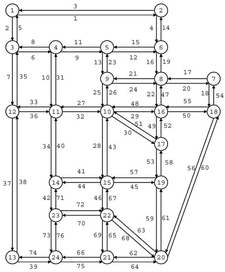
Figure 1.
Sioux Falls Network. Source: [64].
The kind of membership function used in this FL model must be specified. Data structure distribution and expert validation are considered in this process. The authors chose triangular membership functions to prove their models. Thus, this membership function is more than enough, and it is the best way to test the model because of its simplicity. Due to the function’s shape, it should define the three vertices’ values, which define the limit values for every constraint, where they can oscillate. The vertical measure indicates the λ value or the accomplishment level achieved using specialized software to run the models and to test the formulations proposed in this paper. The models were run as continuous problems. The code was written using GAMS® (General Algebraic Modeling System). This program package includes the mathematical model obtained, the flexible parameters, the membership functions, and the input data (costs, volume in links, tour production in nodes).
The TTS using the fuzzy parameter formulation was developed in Section 3. To test the model, the numerical application also used the SF network. Data were created for this research, which are 15 transit tour sequences (routes). The tours were randomly generated, using three nodes as origin nodes, and each node served as the origin of five tours. The bus tours seek to cover different types of routes, including rounded and the whole perimeter of the network, and other more partitioned routes for specific areas, but all nodes were in at least one of the bus tours.
In transit tours, the 24 nodes of the SF network represent the stops made in the stations by the buses during the route, except when a node is the departure and arrival point (tour start and end point), which is considered the tour producer node.
This optimization problem was run using the ε approach. Remember that ε values are in the interval [0, 1], with steps of 0.05. In the beginning, the GAMS results showed ε = 0.4 as the maximum value to obtain feasible solutions. All solutions were unfeasible when the model ran with ε = 0.45 and greater. However, the authors tried using a smaller step size (0.01), from ε = 0.4, just to be closer to the value whereat the feasible solutions stopped. Then, the model was run again for {ε = 0.41, ε = 0.42, ε = 0.43, ε = 0.44}; when we used ε = 0.43, the solution became unfeasible, and the same for greater values. Then, the model obtained feasible solutions for values less than ε = 0.43. In other words, as a minimum, a constraint determines at least 43% of the objective value. This result for transit formulation shows a λ value of λ = 0.42. The results are associated with the data in any case.
Figure 2 shows a graphic of entropy values vs. the level of accomplishment. Remember the x-axis is the minimum accomplishment level obtained, that is, the constraint that fared the worst. Conversely, the y-axis corresponds to the maximum entropy obtained in each solution.
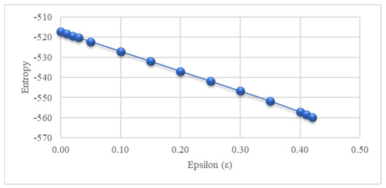
Figure 2.
Transit Pareto frontier (entropy vs. accomplishment level).
Figure 2 shows that the entropy-based TTS formulation using FL is a multi-objective optimization problem, since both variables are opposite each other, in competition. With each increment in the accomplishment level, the entropy decreases. That is, the proof that exists is, in this case, the Pareto frontier for the data used. This result is relevant to this paper’s main objective: that the formulations using fuzzy parameters are useful methodologies, and results always depend on the input data. When the variability of the data is high, the λ value is low, and if the variability is smaller, the uncertainty in the model also is, and the λ value increases, that is, the accomplishment level also increases.
Every feasible solution gives the number of buses that use every tour, that is, the bus tour flows. Thus, the flow changes between the tours and for every ε-value. Figure 3 shows these changes in the traffic, from the minimum ε-value, until the λ value. In this experiment, it seems that most of the tours show increments between 5% and 10% of the flow, without much change, and the data variability is not very strong. The results also present moderate variability.
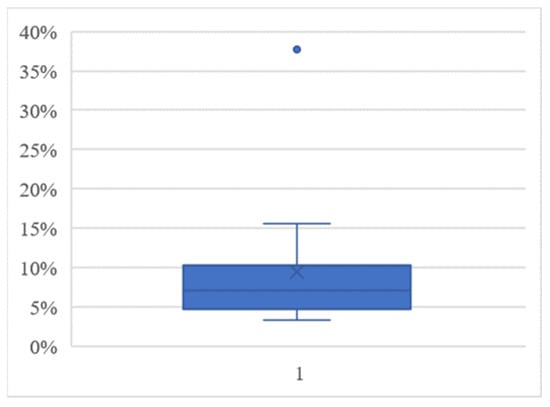
Figure 3.
Bus traffic changes for each different solution.
Figure 4. The changes in the flow in every tour.
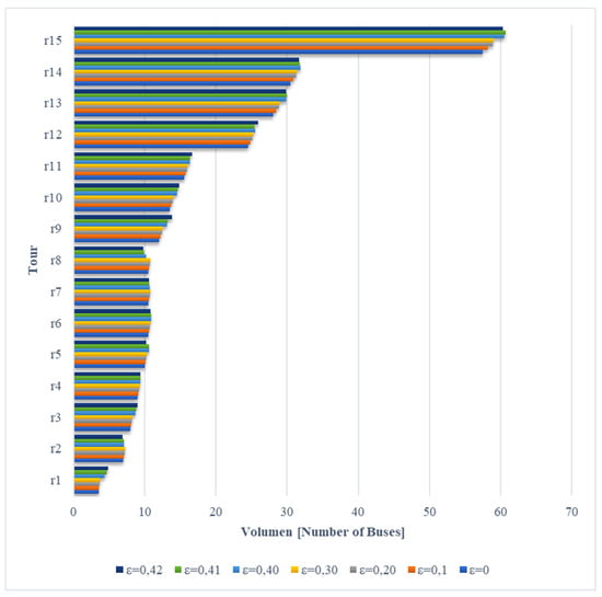
Figure 4.
Bus tour volumes for different ε values.
The graphic exhibits the number of buses per tour for different ε values. Due to the small amount of transit data used in this experiment, the graphic includes all tours. We can see the changes in every tour, in every solution. It is possible to see that the changes are soft, and most keep the tendency in every tour. However, tours 1 and 15 exhibited greater changes than the rest—mainly tour 15, which shows increased bus flow as the level of compliance increased. Tour 8 showed the opposite circumstance; when compliance levels increased, the number of buses on the tour tended to decline. Including fuzzy parameters brings flexibility to the constraints; this influences the results of the solution related to the volume pattern changes of the tours, since it prevents identifying the tendency of those changes.
The results for the different solutions give as output the percentage or level of accomplishment per tour at every ε value evaluated in the model. This can be better understood with a graphic such as that in Figure 5.
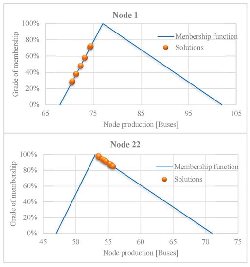
Figure 5.
TTS level (%) of accomplishment in nodes production.
It shows two nodes, node 1 and node 22, and their respective triangular membership functions with the solution obtained at every ε value tested. That is, on the x-axis is the number of buses using the node every tour, and on the y-axis is the respective grades of accomplishment. The results show that levels of accomplishment are related to the node-production twice in every tour. This must be understood in relation to the triangle side on which the solution is. The left side shows that the number of buses obtained is lower than the required value, while the right side shows that the number of buses obtained is more than the required value. Following this, Figure 5 shows that while node 1’s tour production is less than required, node 22 produces more bus tours than required. This analysis allows for comparing the production per node per tour. In the case of links, the same analysis shows the volume per link per tour, and every constraint using fuzzy parameters.
The side vertices of the triangular membership functions correspond to the extreme production and grade of accomplishment values. This is due, in both cases, to the fact that the grade of accomplishment is 0% (zero). If the solution is the minimum interval value, the left extreme means that the constraint is at least 0%, and this is the worst case. Others may be in the same condition, or better. The solution is specific to the constraint evaluated, and independent of the others.
Figure 6 and Figure 7 represent the percentage of accomplishment for each tour and its distribution for both node-production and link-volume, respectively. Note that the minimum accomplishment value is equal to the ε-value in every solution, whereas the other constraints achieve higher values of accomplishment, even 100%.
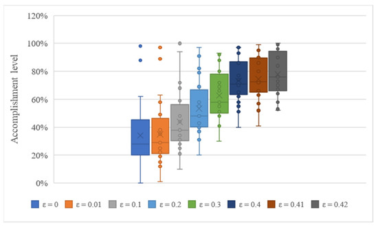
Figure 6.
TTS percentage accomplishment in node-production constraint.
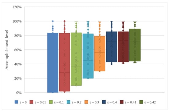
Figure 7.
TTS percentage accomplishment in link-volume constraint.
Despite the tours’ fluctuation in both figures, there was a significant difference between each solution, and none of the solutions exhibited this tendency.
Table 1 shows the number of accomplishments with minimum and maximum values and other statistics for node-production and link-volume constraints. The table shows the observations of the statistical values. While the variation per solution (every ε-value) is strong, the results of the tours inside the same solution have a homogeneous tendency. For the case of the ε = 0.3 solutions, the tour’s average compliance relative to the production constraint (on the 24 nodes) was 63%, with a standard deviation of 0.17, while in the case of the volume constraint (on the 76 links) the tour’s average compliance was 58%, with a standard deviation of 0.24. In both production and volume, the minimum compliance value is equal to the respective ε-value, just as expected.

Table 1.
TTS descriptive analysis of accomplishment.
This numerical experiment’s objective is to validate the methodology proposed in this research, applying the formulation to estimate transit (bus) tours based on entropy maximization using fuzzy parameters. The Pareto frontier is specific to every case study, given that it depends on every data set. That is, every replication of the experiment will have its own Pareto frontier; it could get a better or worse λ value. In this case, λ = 0.15 for freight and λ = 0.42 for transit, and these results correspond only to the specific case study.
In a few words, the numerical experiments consisted of running the model using several values for ε between 0 and 1 each time. What is common is that, at a certain point, the run stops giving feasible solutions, and starts giving infeasible solutions from then on. In the experiment, those solutions were discarded, and only the ε values that deliver feasible results were preserved. The λ parameter, in FL theory, can take values between 0 and 1, and represents the membership percentage for every solution. This is the reason for running the model several times using different ε parameter values (minimum allowed value for the λ parameter), starting from 0 with steps of 0.01 in FTS and 0.05 in TTS. The ε value means that at least a constraint (but it can be more) gets a membership value or accomplishment of ε%. Lower values of ε are reflected in the model’s flexibility because it offers the chance to partially accomplish the constraints.
The running optimization process, as explained earlier, works using the ε approach, where ε is an input parameter; ε ∈ [0, 1], using a triangular membership function. The upper vertex of the triangle represents the requested (goal or target) value corresponding to the deterministic values obtained after assignment stage. This means that the requested values are those values given when ε = 1; since these are unfeasible solutions, “the term ‘satisfying solution’ suits better than ‘optimal solution’” [65], meaning that in the flexibilization of the program, we gain a “satisfying solution”, instead of an optimal solution.
Comparison FL Model and No FL Models Solutions
To demonstrate if the flexible solution really is better than the deterministic solution of the problem, the EM-based model was run using a deterministic form of the model, using, instead of flexibility constraints (for both production and volume), FL and fixed parameters in constraints, which constitutes the deterministic model. In such cases, the solution was not feasible, making the formulation with FL better than deterministic. Additionally, the problem was run several times in order to determine the results of relaxing the parameter productions and volume, one by one and simultaneously. To do so, we created an indicator (Δ) that measures the distance between the model’s obtained solution and the requested value or target value (the upper value signed by the middle triangle vertex), corresponding to λ = 1. We called this indicator “Distance from the target value (Δ)”, and it was calculated for both production and volume constraints.
The mentioned relaxations consider different scenarios. (1) Taking only production constraint and relaxing it as a greater-than inequality and as a lower-than inequality; (2) taking only the volume constraint and relaxing it as a greater-than inequality and as a lower-than inequality; (3) taking both production and volume constraints and relaxing them as greater-than inequalities, and as lower-than inequalities, for a total of six different scenarios in the case of the nodes (tours generation) and six in the case of the links (volume). All those cases were compared with this paper’s proposed solution, which used FL parameters, and according to which the best performance was for ε = 0.42.
Production constraint Δ is defined as follows:
where
- —Difference from the requested value for production (nodes);
- —Obtained production value from solution;
- —Production requested value.
Analogously, the Δ for volume is defined as follows:
where
- —Difference from the requested value for volume (links);
- —Obtained volume value from solution;
- —Volume requested value.
In all the models, the proposed flexible model, and the six described comparison scenarios, the percentage distance of the solution was measured, in each case, with respect to the target value of production and volumes. Table 2 presents those differences on the flow in every link, and Table 3 contains descriptive information for every scenario. This comparison allows us to observe how all scenarios, compared with the flexibilizated problem (named FL Model in the tables), have greater distances from the target solution (Δ) than the FL model. We can observe for instance that Link 1 (A1) in Table 2 tell us that none of the relaxed problems (case 1 to case 6 in the table) give a smaller distance from the target value than the one obtained in the flexible model (FL model in the table), which means that the use of the fuzzy parameters undoubtedly improves the performance of the model, with better solutions.
Table 2.
Percentage distance from the target value (ΔVa) of the flow per link.
Table 3.
Percentage distance (ΔVa) descriptive links (volume).
The descriptive information presented in Table 3 shows that the FL model’s average, for volumes, is closer to the requested value than any other case for the volumes. In other words, in the FL model, the average ΔVa is the smallest in the comparison process, and in other cases, for example, Case 2, ΔVa achieved 91%. Moreover, P75 exhibited the same behavior, and again the FL model achieved ΔVa = 7%, while the rest of the scenarios were all over 11%.
The situation in the case of the nodes (production) analysis shows a similar structure. As in the case of the links, in the nodes, the indicator ΔOi is greater in the evaluated scenarios than in the flexible problem. This result is noted in Table 4 and Table 5.
Table 4.
Percentage distance from the target value (ΔOi) of the production per node.
Table 5.
Percentage distance (ΔOi) descriptive nodes (production).
The percentage distance for production ΔOi obtained using this study’s proposed model corresponds on average to 3% with respect to the target or requested value, and that is the smallest value obtained for cases 1 to 6. As this result is consistent with the hypothesis of this investigation, it is possible to affirm than the flexible solution obtained from the EM-based model using FL parameters is much better than the deterministic cases.
5. Conclusions and Discussion
One of the main worries in planning is daily uncertainty, because capturing it is a very difficult issue. When decision-makers can control the uncertainty levels, the probability of success increases. The inclusion of FL in the transport modeling process is barely understood and rarely used, even when it has shown its ability by reducing the gap between modeling and reality (but not eliminating it).
This research proposes using fuzzy parameters for estimating tour flows, using traffic counts to be solved with entropy maximization techniques for transit (buses). The paper presents and tests the entropy-based TTS using FL, which is a newly proposed formulation for modeling transit (buses) using the same technique, which, to the author’s best knowledge, is a contribution to the literature. The FL applied to the formulation is based on membership functions and the ε approach. In this research, the triangular membership functions, which are the simplest and very common, were used, given that they show the most common distribution in data; as such, this function is frequently chosen by experts. This paper addresses a numerical experiment in the Sioux Falls network.
Some cases exist wherein a feasible solution corresponds to the lowest values for ε in the minimum value of membership. This condition implies that the nonflexible problem does not have a feasible solution with the constraints used. Nevertheless, a partial solution is better than nothing for practitioners. The proposed method allows for obtaining the best solution possible when a total accomplishment of each constraint is not possible.
The indicator “Distance from the target value (Δ)” was created to measure the distance between the model’s obtained solution and the requested value or target value, which corresponds to λ = 1. It was calculated for both production and volume constraints. The problem was run several times in seeking to determine the resultant solutions of relaxing the parameters of productions and volume, one by one and simultaneously. All those cases were compared with this paper’s model’s proposed solution, in which the best performance was with ε = 0.42. For both production and volume, the FL model had smaller Δ values than the ones obtained in the no FL models, which means that the use of the fuzzy parameters undoubtedly improves the performance of the model, with better solutions. In a few of the links or nodes, some of the comparative cases scenarios could achieve a better Δ, but these are not relevant when in general most of them present strong differences in the indicator. When considering what is real, it is not always possible to fully comply with constraints. Planners and decision-makers must try to find an equilibrium, and these formulations can contribute to that point, decreasing the level of uncertainty. This is because the FL model allows one to obtain “satisfying solutions” instead of no solutions, when the deterministic problem is unfeasible. The inclusion of fuzzy logic with the entropy maximization approach to estimate bus tour flows significantly improves the quality of the results.
This methodology can generate helpful information for decision-makers. The solutions obtained can effectively represent the natural behavior of transit or any other problem. The FL is a powerful tool when a problem implies variability and uncertainty. It could build better transportation planning systems for agencies to improve mobility in cities and urban areas. Moreover, FL helps include the parameter variability inherent in daily life in the input data, which should also be reflected in the outputs. The obtained results are more reliable because of the more realistic shapes of the models.
The Pareto frontier, obtained from a comparison of the entropy, shows that while entropy decreases, the ε value increases, which means that the problem is multi-objective. Thus, considering the number of vehicles when using the links to obtain comparable entropy values is necessary.
This research used FL to make the corresponding constraints in node-production and link-volume flexible. However, the authors found that the link cost can also be flexible in other research areas (i.e., considering congestion). Future research should include better forms of the membership function applied to constraint flexibilization.
Author Contributions
The authors confirm the following contributions to the paper. Conceptualization, D.P.M.-P., C.A.G.-C. and J.J.P.-H. Methodology, D.P.M.-P., C.A.G.-C. and H.L.-O. Software, D.P.M.-P., H.L.-O. and J.K.G.-M. Validation, D.P.M.-P., C.A.G.-C., H.L.-O. and J.K.G.-M. Formal analysis, D.P.M.-P., C.A.G.-C., H.L.-O. and J.K.G.-M. Investigation, D.P.M.-P., C.A.G.-C. and J.J.P.-H. Resources, D.P.M.-P. Data curation, D.P.M.-P. Writing—original draft preparation, D.P.M.-P. Writing—review and editing, C.A.G.-C., J.J.P.-H., H.L.-O. and J.K.G.-M. Visualization, D.P.M.-P. and C.A.G.-C. Supervision, C.A.G.-C. and J.J.P.-H. Project administration, C.A.G.-C. All authors have read and agreed to the published version of the manuscript.
Funding
This research received no external funding.
Institutional Review Board Statement
Not applicable.
Informed Consent Statement
Not applicable.
Data Availability Statement
Not applicable.
Conflicts of Interest
The authors declare no conflict of interest.
References
- Nagy, A.; Ercsey, Z.; Tick, J.; Kovács, Z. Bus transport process network synthesis. Acta Polytechnica Hungarica 2019, 16, 25–43. [Google Scholar] [CrossRef]
- Wirasinghe, S.C.; Kattan, L.; Rahman, M.M.; Hubbell, J.; Thilakaratne, R.; Anowar, S. Bus rapid transit—A review. Int. J. Urban Sci. 2013, 17, 1–31. [Google Scholar] [CrossRef]
- Soehodo, S.; Koshi, M. Design of public transit network in urban area with elastic demand. J. Adv. Transp. 1999, 33, 335–369. [Google Scholar] [CrossRef]
- Fan, W.; Machemehl, R.B. Optimal Transit Route Network Design Problem with Variable Transit Demand: Genetic Algorithm Approach. J. Transp. Eng. 2006, 132, 40–51. [Google Scholar] [CrossRef]
- Lam, W.; Gao, Z.; Chan, K.; Yang, H. A stochastic user equilibrium assignment model for congested transit networks. Transp. Res. Part B Methodol. 1999, 33, 351–368. [Google Scholar] [CrossRef]
- De Cea, J.; Fernández, E. Transit Assignment for Congested Public Transport Systems: An Equilibrium Model. Transp. Sci. 1993, 27, 133–147. [Google Scholar] [CrossRef]
- Spiess, H.; Florian, M. Optimal strategies: A new assignment model for transit networks. Transp. Res. Part B Methodol. 1989, 23, 83–102. [Google Scholar] [CrossRef]
- Wu, J.H.; Florian, M.; Marcotte, P. Transit Equilibrium Assignment: A Model and Solution Algorithms. Transp. Sci. 1994, 28, 193–203. [Google Scholar] [CrossRef]
- Lam, W.H.K.; Wu, Z.X.; Chan, K.S. Estimation of Transit Origin–Destination Matrices from Passenger Counts Using a Frequency-Based Approach. J. Math. Model. Algorithms 2003, 2, 329–348. [Google Scholar] [CrossRef]
- López-Ospina, H.; Cortés, C.E.; Pérez, J.; Peña, R.; Figueroa-García, J.C.; Urrutia-Mosquera, J. A maximum entropy optimization model for origin-destination trip matrix estimation with fuzzy entropic parameters. Transp. A Transp. Sci. 2021, 18, 963–1000. [Google Scholar] [CrossRef]
- Kepaptsoglou, K.; Karlaftis, M. Transit Route Network Design Problem: Review. J. Transp. Eng. 2009, 135, 491–505. [Google Scholar] [CrossRef]
- Nielsen, O.A. A stochastic transit assignment model considering differences in passengers utility functions. Transp. Res. Part B Methodol. 2000, 34, 377–402. [Google Scholar] [CrossRef]
- Lam, W.H.; Zhou, J.; Sheng, Z.-H. A capacity restraint transit assignment with elastic line frequency. Transp. Res. Part B Methodol. 2002, 36, 919–938. [Google Scholar] [CrossRef]
- Abdulaal, M.; LeBlanc, L.J. Continuous equilibrium network design models. Transp. Res. Part B Methodol. 1979, 13, 19–32. [Google Scholar] [CrossRef]
- Chakirov, A.; Fourie, P.J. Enriched Sioux Falls scenario with dynamic and disaggregate demand. Arb. Verk. Raumplan. 2014, 978, 385–386. [Google Scholar]
- Willumsen, L.G. Estimation of an OD Matrix from Traffic Counts—A Review; Institute of Transport Studies, University of Leeds: Leeds, UK, 1978. [Google Scholar]
- Wong, S.C.; Tong, C.O.; Wong, K.I.; Lam, W.H.K.; Lo, H.K.; Yang, H. Estimation of Multiclass Origin-Destination Matrices from Traffic Counts. J. Urban Plan. Dev. 2005, 131, 19–29. [Google Scholar] [CrossRef]
- Willumsen, L.G. OD matrices from network data: A comparison of alternative methods for their estimation. In Proceedings of the PTRC Summer Annual Meeting 1978 Seminar in Transport Models, Leeds, UK, 1978. [Google Scholar]
- Willumsen, L.G. Estimation of Trip Matrices from Volume Counts. Validation of a Model under Congested Conditions; University of Leeds: Leeds, UK, 1982. [Google Scholar]
- Willumsen, L.G. Estimating Time-Dependent Trip Matrices from Traffic Counts. In Proceedings of the Ninth International Symposium on Transportation and Traffic Theory, Delft, The Netherlands, 11–13 July 1984; pp. 397–412. [Google Scholar]
- Abrahamsson, T. Estimation of Origin-Destination Matrices Using Traffic Counts—A Literature Survey; IIASA: Laxenburg, Austria, 1998. [Google Scholar]
- Ortúzar, J.D.D.; Willumsen, L.G. Modelling Transport, 4th ed.; John Wiley & Sons, Ltd.: Hoboken, NJ, USA, 2011. [Google Scholar] [CrossRef]
- Gonzalez-Calderon, C.A. Multiclass Equilibrium Demand Synthesis; Rensselaer Polytechnic Institute: Troy, NY, USA, 2014. [Google Scholar]
- Gonzalez-Calderon, C.A.; Holguín-Veras, J. Entropy-based freight tour synthesis and the role of traffic count sampling. Transp. Res. Part E Logist. Transp. Rev. 2019, 121, 63–83. [Google Scholar] [CrossRef]
- Holguín-Veras, J.; Amaya-Leal, J.; Wojtowicz, J.; Jaller, M.; González-Calderón, C.; Sánchez-Díaz, I.; Wang, X.; Haake, D.G.; Rhodes, S.S.; Frazier, R.J.; et al. Improving Freight System Performance in Metropolitan Areas: A Planning Guide; Transportation Research Board: Washington, DC, USA, 2015. [Google Scholar] [CrossRef]
- Wang, Q.; Holguin-Veras, J. Tour-Based Entropy Maximization Formulations of Urban Commercial Vehicle Movements. In Proceedings of the 2009 Annual Meeting of the Transportation Research Board, Washington, DC, USA, 11–15 January 2009; pp. 1–22. [Google Scholar]
- Sánchez-Díaz, I.; Holguín-Veras, J.; Ban, X. A time-dependent freight tour synthesis model. Transp. Res. Part B Methodol. 2015, 78, 144–168. [Google Scholar] [CrossRef]
- Moreno-Palacio, D.P.; Gonzalez-Calderon, C.A.; López-Ospina, H.; Gil-Marin, J.; Posada-Henao, J.J. POMS-2022-Conference Program book. In Freight Tour Synthesis Based on Entropy—Fuzzy Logic; Production and Operations Management Society (POMS): Hong Kong, China, 2022; p. 147. [Google Scholar] [CrossRef]
- Sun, C.; Chang, Y.; Shi, Y.; Cheng, L.; Ma, J. Subnetwork Origin-Destination Matrix Estimation Under Travel Demand Constraints. Networks Spat. Econ. 2019, 19, 1123–1142. [Google Scholar] [CrossRef]
- Velichko, A. Interregional Transportation Modeling for the Far East of Russia Macro-region. In Proceedings of the 9th International Conference on Discrete Optimization and Operations Research and Scientific School, Vladivostok, Russia, 19–23 September 2016; pp. 394–403. [Google Scholar]
- Tang, J.; Zhang, S.; Chen, X.; Liu, F.; Zou, Y. Taxi trips distribution modeling based on Entropy-Maximizing theory: A case study in Harbin city—China. Phys. A Stat. Mech. Appl. 2018, 493, 430–443. [Google Scholar] [CrossRef]
- Hewings, G.J.D.; Fernandez-Vazquez, E. Entropy maximization and input–output analysis. Interdiscip. Sci. Rev. 2019, 44, 272–285. [Google Scholar] [CrossRef]
- Hu, B.; Ma, Y.; Pei, Y.; Gao, W. Statistical analysis and predictability of inter-urban highway traffic flows: A case study in Heilongjiang Province, China. Transp. A Transp. Sci. 2020, 16, 1062–1078. [Google Scholar] [CrossRef]
- Nguyen, S.; Pallottino, S. Equilibrium traffic assignment for large scale transit networks. Eur. J. Oper. Res. 1988, 37, 176–186. [Google Scholar] [CrossRef]
- Wong, S.; Tong, C. Estimation of time-dependent origin–destination matrices for transit networks. Transp. Res. Part B Methodol. 1998, 32, 35–48. [Google Scholar] [CrossRef]
- Nuzzolo, A.; Crisalli, U. Estimation of transit origin/destination matrices from traffic counts using a scheduled-based approach. In Proceedings of the European Transport Forum 2001, Cambridge, UK, 2001. [Google Scholar]
- Fisk, C. Trip matrix estimation from link traffic counts: The congested network case. Transp. Res. Part B Methodol. 1989, 23, 331–336. [Google Scholar] [CrossRef]
- Zadeh, L.A. Fuzzy sets. Inf. Control 1965, 8, 338–353. [Google Scholar] [CrossRef]
- Zadeh, L.A. Fuzzy algorithms. Inf. Control 1968, 12, 94–102. [Google Scholar] [CrossRef]
- Hannan, E.L. Linear programming with multiple fuzzy goals. Fuzzy Sets Syst. 1981, 6, 235–248. [Google Scholar] [CrossRef]
- Zimmermann, H.-J. Fuzzy programming and linear programming with several objective functions. Fuzzy Sets Syst. 1978, 1, 45–55. [Google Scholar] [CrossRef]
- Sakawa, M. Interactive Fuzzy Decision Making for Multiobjective Linear Programming Problems and its Application. IFAC Proc. Vol. 1983, 16, 295–300. [Google Scholar] [CrossRef]
- Sakawa, M.; Yano, H. An Interactive Fuzzy Satisficing Method for Multiobjective Linear Programming Problems with Fuzzy Parameters. IFAC Proc. Vol. 1987, 20, 437–442. [Google Scholar] [CrossRef]
- Bellman, R.; Zadeh, L.A. Decision-Making in a Fuzzy Environment. Manag. Sci. 1970, 17, B141–B164. [Google Scholar] [CrossRef]
- Zadeh, L.A. Fuzzy sets as a basis for a theory of possibility. Fuzzy Sets Syst. 1999, 100, 9–34. [Google Scholar] [CrossRef]
- Bit, A.; Biswal, M.; Alam, S. Fuzzy programming approach to multicriteria decision making transportation problem. Fuzzy Sets Syst. 1992, 50, 135–141. [Google Scholar] [CrossRef]
- Chanas, S.; Kuchta, D. A concept of the optimal solution of the transportation problem with fuzzy cost coefficients. Fuzzy Sets Syst. 1996, 82, 299–305. [Google Scholar] [CrossRef]
- Aggarwal, M. Redefining fuzzy entropy with a general framework. Expert Syst. Appl. 2020, 164, 113671. [Google Scholar] [CrossRef]
- López-Ospina, H. Modelo de maximización de la entropía y costos generalizados intervalares para la distribución de viajes urbanos. Ing. Univ. 2013, 17, 390–407. [Google Scholar]
- Zhang, Y.; Ye, Z. Short-Term Traffic Flow Forecasting Using Fuzzy Logic System Methods. J. Intell. Transp. Syst. 2008, 12, 102–112. [Google Scholar] [CrossRef]
- Majidi, S.; Hosseini-Motlagh, S.-M.; Yaghoubi, S.; Jokar, A. Fuzzy green vehicle routing problem with simultaneous pickup—Delivery and time windows. RAIRO Oper. Res. 2017, 51, 1151–1176. [Google Scholar] [CrossRef]
- Tamin, O.Z.; Willumsen, L.G. Freight Demand Model Estimation from Traffic Counts. Simpl. Transp. Demand Model. 1992, 75–86. [Google Scholar]
- Holguín-Veras, J.; Encarnación, T.; Ramírez-Ríos, D.; He, X.; Kalahasthi, L.; Pérez-Guzmán, S.; Sanchez-Díaz, I.; González-Calderón, C.A. A Multiclass Tour Flow Model and Its Role in Multiclass Freight Tour Synthesis. Transp. Sci. 2020, 54, 631–650. [Google Scholar] [CrossRef]
- Wilson, A.G. The use of entropy maximising models, in the theory of trip distribution, mode split and route split. J. Transp. Econ. Policy 1969, 3, 108–126. [Google Scholar]
- Leblanc, L.J.; Morlok, E.K.; Pierskalla, W.P. An efficient approach to solving the road network equilibrium traffic assignment problem. Transp. Res. 1975, 9, 309–318. [Google Scholar] [CrossRef]
- Suwansirikul, C.; Friesz, T.L.; Tobin, R.L. Equilibrium Decomposed Optimization: A Heuristic for the Continuous Equilibrium Network Design Problem. Transp. Sci. 1987, 21, 254–263. [Google Scholar]
- Friesz, T.L.; Cho, H.-J.; Mehta, N.J.; Tobin, R.L.; Anandalingam, G. A Simulated Annealing Approach to the Network Design Problem with Variational Inequality Constraints. Transp. Sci. 1992, 26, 18–26. [Google Scholar] [CrossRef]
- Marcotte, P.; Marquis, G. Efficient implementation of heuristics for the continuous network design problem. Ann. Oper. Res. 1992, 34, 163–176. [Google Scholar] [CrossRef]
- Meng, Q.; Yang, H.; Bell, M. An equivalent continuously differentiable model and a locally convergent algorithm for the continuous network design problem. Transp. Res. Part B Methodol. 2001, 35, 83–105. [Google Scholar] [CrossRef]
- Lee, S.; Lim, J. Effectiveness and Macroeconomic Impact Analysis Of Policy Instruments For Sustainable Transport In Korea: A CGE Modelling Approach. WIT Transac. Built Environ. 2002, 60, 1–12. [Google Scholar]
- Josefsson, M.; Patriksson, M. Sensitivity analysis of separable traffic equilibrium equilibria with application to bilevel optimization in network design. Transp. Res. Part B Methodol. 2007, 41, 4–31. [Google Scholar] [CrossRef]
- Luathep, P.; Sumalee, A.; Lam, W.H.; Li, Z.-C.; Lo, H.K. Global optimization method for mixed transportation network design problem: A mixed-integer linear programming approach. Transp. Res. Part B Methodol. 2011, 45, 808–827. [Google Scholar] [CrossRef]
- Bar-Gera, H.; Hellman, F.; Patriksson, M. Computational Precision of Traffic Equilibria Sensitivities in Automatic Network Design and Road Pricing. Procedia Soc. Behav. Sci. 2013, 80, 41–60. [Google Scholar] [CrossRef]
- Wei, X.; Yu, W.; Wang, W.; Zhao, D.; Hua, X. Optimization and Comparative Analysis of Traffic Restriction Policy by Jointly Considering Carpool Exemptions. Sustainability 2020, 12, 7734. [Google Scholar] [CrossRef]
- Luhandjula, M. Fuzzy optimization: Milestones and perspectives. Fuzzy Sets Syst. 2015, 274, 4–11. [Google Scholar] [CrossRef]


Publisher’s Note: MDPI stays neutral with regard to jurisdictional claims in published maps and institutional affiliations. |
© 2022 by the authors. Licensee MDPI, Basel, Switzerland. This article is an open access article distributed under the terms and conditions of the Creative Commons Attribution (CC BY) license (https://creativecommons.org/licenses/by/4.0/).