Evaluating Spatiotemporal Variations of Groundwater–Surface Water Interaction Using an Integrated Hydrological Model in Huashan Basin, China

Abstract

Quantifying the spatiotemporal variations of basin-scale surface water (SW)–groundwater (GW) interactions is vital for the conjunctive management of water resources in the basin. In this study, an integrated hydrological model (SWAT-MODFLOW) is used to simulate the SW–GW system in the Huashan Basin. The numerical model was calibrated and validated using the streamflow observations of the watershed outlet and the groundwater levels of the long-term monitoring wells from 2016 to 2020 in the study area. The model results show that the SWAT–MODFLOW can achieve a better fit for the streamflow discharge, compared with the results in the single SWAT model, with R² (coefficient of correlation) and NSE (Nash-Sutcliffe efficiency coefficient) of 0.85 and 0.83, respectively. The water table fitting results indicate that R² and RMSE can reach 0.95 and 0.88, respectively. The water budgets analysis demonstrates that the average rate (0.5281 m³/s) of GW abstraction to SW is larger than the rate (0.1289 m³/s) of SW recharge to GW. Moreover, the exchange rate of SW and GW gradually reaches a peak value from June to August, and the lowest value is shown in April, for each hydrological year. Based on the IPPC6 CanESM5 dataset supplied by the Canadian Climate Centre, the regional precipitation scenario subject to climate change was predicted by the ASD (Auto Statistical Downscaling Model) a statistical downscaling method, under the climate scenarios of SSP2_4.5 and SSP5_8.5. The SW–GW interaction pattern was modeled under the future scenarios in the study area. The current (2016–2020) average annual rate of the SW–GW interaction is considered as the base value. Subject to the SSP2_4.5 scenario, the average exchange rate of the SW recharge to GW is 0.1583 m³/s, which is an increase of 22.8%. The average exchange rate of the GW discharge to SW is 0.5189 m³/s which is a reduction of 0.017%. Subject to the SSP5_8.5 scenario, the average exchange rate of SW recharge to GW is 0.1469 m³/s, which is an increase of 14.7%. The average exchange rate of the GW discharge to SW is 0.5953 m³/s, which is an increases of 12.7%. The results can assist in water resource management in the basin, by identifying potential locations of nutrient transport from the aquifer to the river, as well as changes in spatial variability under future climatic conditions.

1. Introduction

The interactions between surface water and groundwater affect the water recharge–discharge, water supply, pollutant discharge and water ecology of a watershed system [1,2,3,4], and the utilization of any of this water will impact the whole water resources system. Hence, water resources assessment should take the surface water and groundwater in a watershed as a whole, within the development of integrated water resources management [5,6]. Furthermore, quantification the surface water–groundwater interaction at the basin scale is of great significance to the sustainable development of water resources.

Focusing on one of the two systems and simplifying the other one, such as with SWAT, TOPMODEL and MODFLOW, and simulating both the surface water system and groundwater system are two commonly used models for analyzing the surface water–groundwater interaction at the basin scale [7,8,9]. The second kind of model consists of the fully coupled models which can simultaneously solve the surface water and groundwater equations, and the loosely coupled models, which solve the surface water and groundwater equations separately and exchange the model results at the boundaries. HydroGeoSphere and MIKE-SHE were the widely used fully coupled models and GSFLOW and SWAT-MODFLOW were the extensively used loosely coupled models [10,11,12,13]. The high demand of data requirement and computational costs were common issues for constructing a fully coupled model at the watershed scale, whereas the loosely coupled model can utilize the current typical surface water and groundwater model, and most software related to it was open-source. Hence, the loosely coupled model was more widely used. Bailey improved the SWAT-MODFLOW coupled model and applied it to the Sprague River watershed in Oregon, U.S.A. The study reproduced the spatial–temporal interaction patterns of surface water–groundwater in the study area from 1970 to 2003 [13]. Jafari constructed a coupled model for the Shiraz watershed in southwestern Italy, and performed a sensitivity analysis of the coupled model [6]. Proloy demonstrated the importance of considering surface water– groundwater interactions in modeling rainfall runoff in southeastern Australia, using a coupled model [7]. Yifru used a coupled model to study groundwater recharge in an agricultural watershed in Korea, and the results can provide a basis for sustainable local water resources development [14].

Since the industrial revolution of the 1860s, global climate change has intensified, and the rate of warming has accelerated. IPCC-AR6 [15] states that in the near-term projections (2021–2040), the global surface 20-year average temperature (GSAT) could increase by 1.5 °C compared to the 1850–1900 average and the high emission scenarios (SSP5-8.5) by 0.9–12.9%, from 1995–2014 (IPCC). Changes in climatic factors such as precipitation and temperature are bound to have profound effects on the water cycle in the basin, especially on the interaction between surface water and groundwater. Therefore, it is necessary to reveal the impact of climate change on surface water–groundwater interactions at the basin scale.

GCMs are the most effective tools for predicting changes in meteorological elements such as climate and hydrology with the increase of greenhouse gases, mainly because GCMs can provide effective information on climate and hydrology research on a global scale [16]. Since the resolution of most current climate models is still not fine enough, there will be large deviations in climate change studies directly applied to regions or watersheds, especially precipitation. Therefore, the downscaling technology plays an unsubstitutable role in climate change research and hydrology research. Statistical downscaling has been widely used in the simulation and prediction of climate variables such as precipitation and temperature, due to its various methods, simplicity and flexibility, and easy construction of a first-level model with a small amount of computation [17]. The two commonly used statistical downscaling methods are regression-based analysis and weather generator-based. Multiple linear regression (MRL) and support vector machine (SVM) are commonly used methods based on regression analysis [18]. SDSM (Statistical Downscaling Model) and ASD are commonly used methods based on weather generators [19,20]. The results of Aimin show that ASD models are able to downscale precipitation with reasonable accuracy [21].

In this study, The Chuzhou hydrological experimental basin was selected and a SWAT-MODFLOW coupled model was constructed, to reproduce the spatial and temporal interaction patterns of surface water– groundwater interactions in the basin. In contrast to previous studies, the coupled model takes into account the spatial distribution of the hydrogeological parameters of the aquifer (permeability coefficients, specific yield), which affect the spatial and temporal variability of the GW; the coupled model also avoids the artificiality of giving the groundwater model a downscaled infiltration coefficient as well as the river bottom and the river level. In addition, the article uses statistical downscaling models to predict future precipitation and temperature in the study area, and analyses the spatial and temporal variability of surface water–groundwater interactions for two future scenarios, SSP2_4.5 and SSP5_8.5, to provide a basis for future water resources development and use in the basin.

2. Methodology

2.1. Study Area

2.1.1. Geography and Climate

The Huashan Basin is located in Chuzhou City, Anhui Province, China. The watershed is located between 118°8′7″ E~118°16′51″ E and 32°13′15″ N~32°18′55″ N. The surface elevation of the watershed is 28 m to 350 m, and the watershed area is about 80 km². The Huashan Basin is surrounded by hills on three sides, with good closure, and has the typical characteristics of Jianghuai hills and landforms. The Chengxi runoff station is the outlet of the Huashan Basin. The study area belongs to the warm temperate semi-humid monsoon climate zone, with an annual average temperature of 15.2 °C. The precipitation is mainly concentrated from June to September, between 610 mm and 1043 mm. The average annual precipitation is 1043 mm. The average annual evaporation is 922 mm.

2.1.2. Hydrology

The river network in the Huashan Basin is fan-shaped, and there are four tributaries above the outlet section, namely Zhuyuangou tributary, Dongyuan tributary, Zhongyuan tributary and Xiyuan tributary. The area of each sub-basin is 2.64 km², 8.82 km², 50.47 km², 17.95 km². The flow of the outlet section has strong seasonality. The precipitation stations and groundwater monitoring wells in the study area are shown in Figure 1. The study area has a low population density, with fewer than 10,000 permanent residents and no centralized mining. The main water supply comes from reservoirs outside the basin.

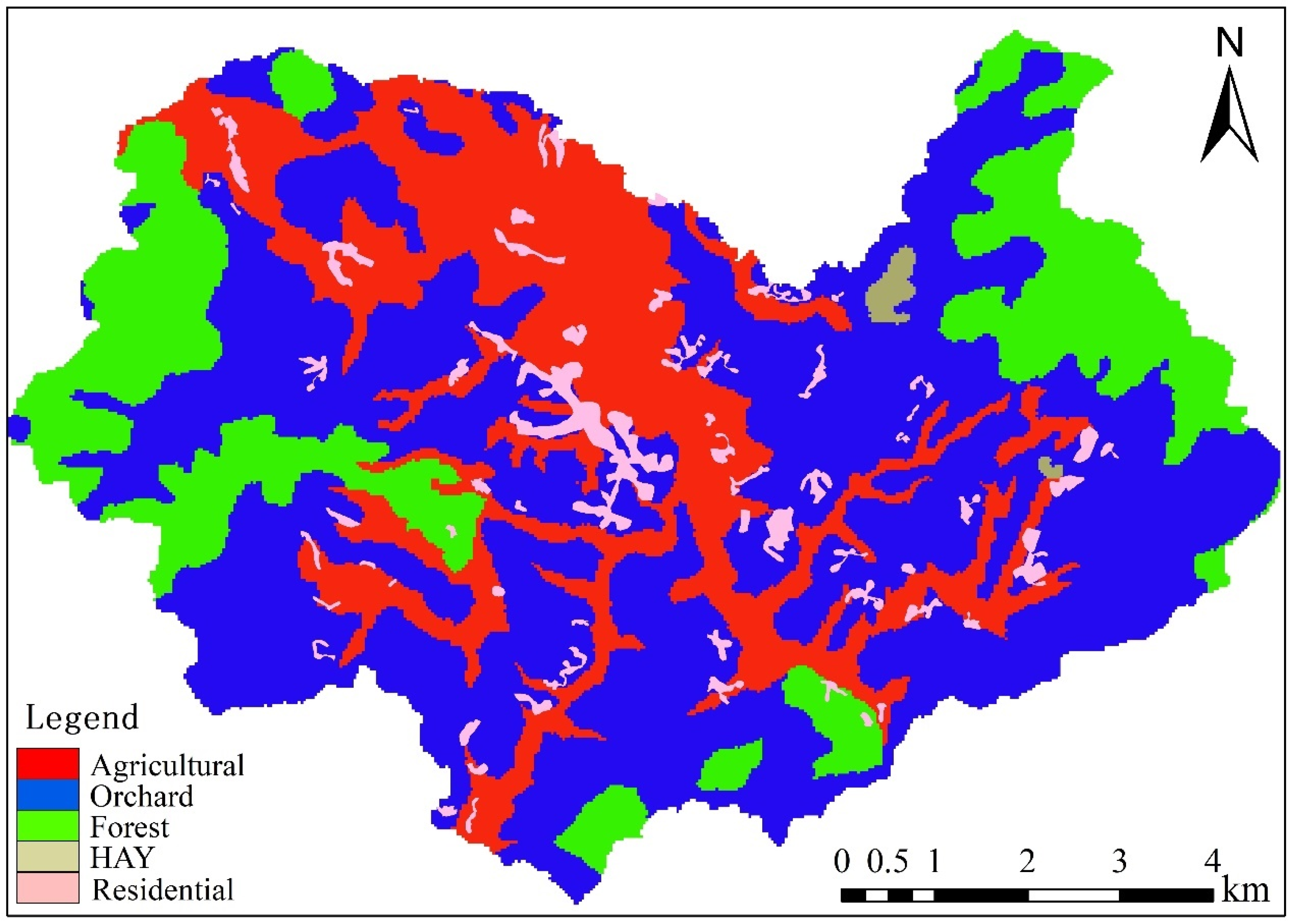
The land-use types in the Huashan Basin are mainly orchard, agriculture and forest, accounting for 51.25%, 24.5% and 17.74%, respectively. The land-use-type map is shown in Figure 2. The soil types are mainly flooded paddy soil and lime soil, and contain a small amount of yellow-brown soil and silico-alumina coarse bone soil. The area of lime soil and flooded paddy soil account for 57.69% and 26.92% of the total area, respectively.

2.1.3. Hydrogeology

The Quaternary aquifer in the Huashan Basin is an unconfined aquifer, and the lithology is mainly silty clay and fine sand, with less gravel. The average thickness of the aquifer is about 7.5 m. Based on the results of the slug tests, the hydraulic conductivity is between 0.5–15 m/d, and the average specific yield is 0.02. The average depth of the groundwater level is 3.5 m, of which the piedmont area is relatively large, with a maximum of 15 m [22]. The surface water–groundwater interaction is frequent in the study area.

2.2. Model

2.2.1. SWAT Model Information

The SWAT model is based on meteorological data, digital elevation, soil type, land-use type and other data, and analyzes the impact of these elements on the transport of water bodies, sediments, and agricultural chemicals. The SWAT model has a strong physical mechanism. It is not represented by a simple linear regression, but fully considers the various processes of the water body on the surface, and needs to input the runoff of the underlying surface and the various information related to the runoff. The model has the advantages of easy access to input data, high computational efficiency, and long-term series simulation. The spatio-temporal resolution and sources of the required data are shown in

Table 1. Data sources and frequency/resolution used for the SWAT model.

Data Type	Date	Frequency/Resolution	Source
DEM	/	12.5 × 12.5 m	Department of Natural Resources of Anhui Province
Land use	2018	30 × 30 m	Department of Natural Resources of Anhui Province
Soil map	/	1 × 1 km	HWSD
Meteorological data	Daily	2000–2020	China Meteorological Data Network
Runoff data	Daily	2016–2020	Chuzhou Hydrology Bureau

. In SWAT, the Huashan Basin is divided into 63 sub-basins and 1136 hydrological response units (HRUs).

2.2.2. MODFLOW Model Information

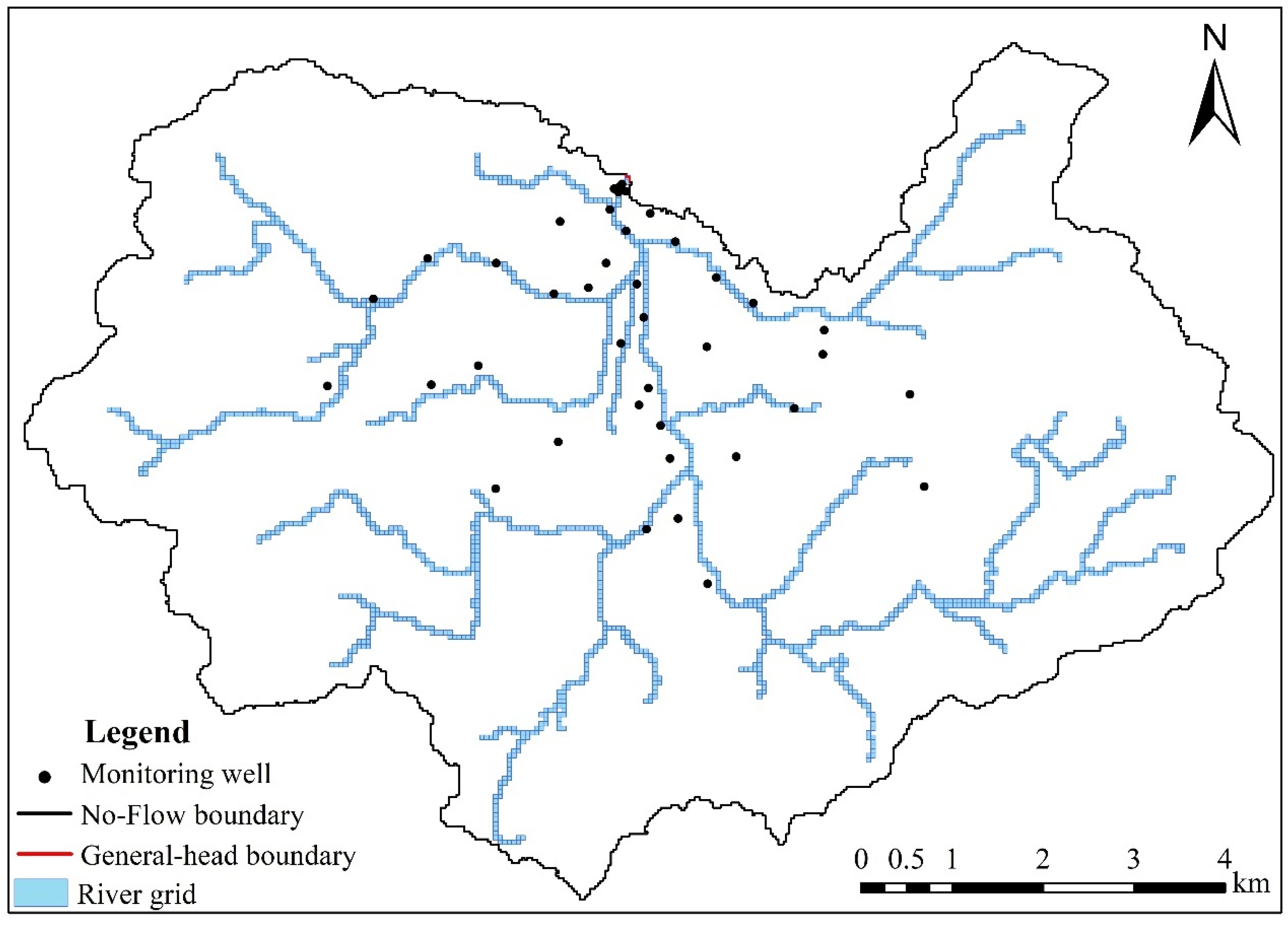
MODFLOW is a fully distributed three-dimensional groundwater flow model based on physical mechanism. It is the most commonly used groundwater flow model. The MODFLOW-NWT version was used. The boundary of the groundwater model is consistent with the boundary of the SWAT model. According to the characteristics of the aquifer, the outlet section is set as the general head boundary, and the rest of the section is set as the no-flow boundary. The top elevation of the model is given by the DEM data. The research area is divided into 189 rows and 275 columns by using 50 m × 50 m unit grids. The vertical pipe experiment was carried out in the riverbed of the Zhongyuan river, and the hydraulic conductivity of the riverbed was small, about 0.005 m/d. In order to provide more accurate initial groundwater levels to facilitate the calibration of the coupled model, a steady flow model was calibrated to provide initial values. The conceptual model of groundwater is shown in Figure 3, below. In MODFLOW, Darcy’s law was used to calculate the interaction between the surface water and groundwater. The formula is as follows [23]:

$$\mathrm{Q}=\mathrm{KLP}\frac{{\mathrm{H}}_{\mathrm{riv}}-{\mathrm{H}}_{\mathrm{gw}}}{\mathrm{Z}}$$

where Q is the interaction flow between the surface water and groundwater (L³/T); K is the hydraulic conductivity of the river bed (L/T); L is the length of the river (L); P is the wet circumference of the river (L); H_riv is the water level of the river (L); H_gw is the groundwater level (L); Z is the thickness of the river bed (L).

2.2.3. SWAT-MODFLOW Model Information

The surface hydrological process is simulated by the SWAT model, which mainly includes the processes of runoff, infiltration, soil moisture evaporation, etc. The groundwater flow is simulated by the MODFLOW-NWT model, including the calculations of the main groundwater source and sink terms such as exploitation, drains and canals and, in addition, the calculation of surface water–groundwater interaction.

Since the HRUs divided by the SWAT have no spatial location information, the HRUs are further decomposed into DHRUs (Disaggregated Hydrologic Response Units) with spatial information, to complete the spatial correspondence between SWAT and MODFLOW. The interaction between the surface water–groundwater is mainly that SWAT transmits the calculated groundwater infiltration recharge to the recharge package of MODFLOW. MODFLOW calculates the interaction between the surface water and groundwater, and transfers it to SWAT. The above process has been integrated into an independent executable program by Professor Bailey from the University of Colorado. MODFLOW is a subroutine of SWAT [13].

2.3. Prediction of Future Precipitation and Temperature

Some research results have shown that the second-generation Canadian Earth System Model (CanESM2) developed by the Canadian Climate Center has achieved good application results in East Asia [24,25,26]. Therefore, the SSP2_4.5 and SSP5_8.5 scenarios provided by the CanESM5 model were selected to predict the future temperature and precipitation in the Huashan Basin.

ASD (Automated Statistical Downscaling model) model is a statistical downscaling model based on the linear regression method, which is developed from the SDSM model (Statistical Downscaling Model) [19]. ASD models rely on the Matlab platform to develop and run, and can automatically select predictors, calibrate model parameters, and generate future climate scenarios. The prediction factor selection method (the recursive algorithm) in the SDSM model was improved. While calculating the partial correlation between two variables, the maximum number of control variables is 12, and the ASD model eliminates the impact of users’ subjective judgment. The specific process of the ASD model has been described in detail in the literature [27].

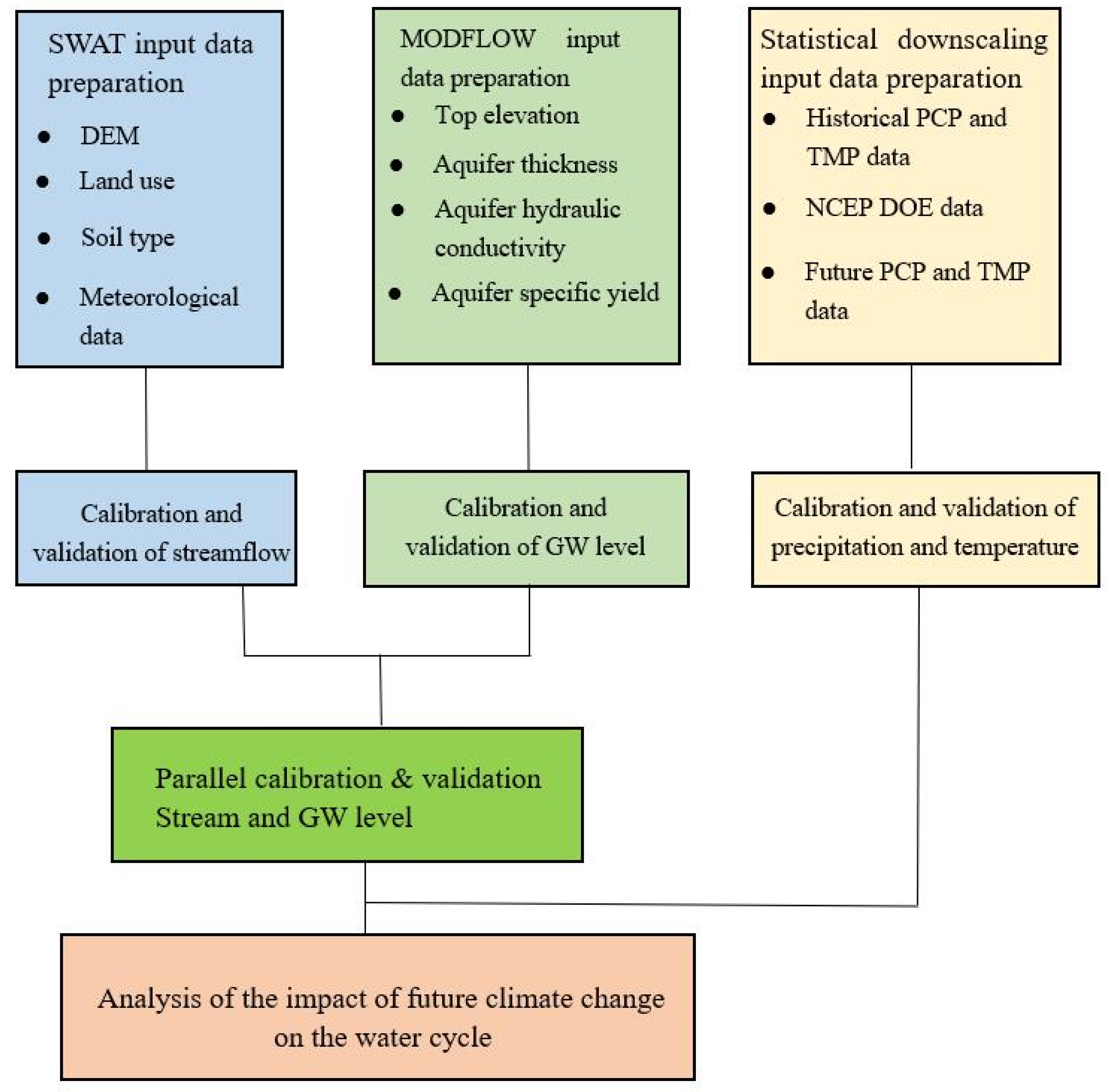
Climate change will affect the surface water–groundwater interaction with the changes of temperature and precipitation in the study area. The atmospheric circulation model and statistical downscaling method are combined to predict the future temperature and precipitation in the study area. The impact of climate change on the spatial-temporal interaction pattern of the surface water and groundwater was analyzed using the SWAT-MODFLOW coupling model in the study area. The coupled model is shown in detail in Figure 4, below. The first step is to use the data of the study area to construct and calibrate the surface-water model and the groundwater model, respectively. The second step is to use the constructed surface-water and groundwater models to calibrate the coupled model. The third step is to prepare meteorological data, using the ASD statistical downscaling model to downscale precipitation and temperature; the fourth step is to input the downscaled data into the coupling model, drive the model, and analyze the results.

3. Result and Discussion

3.1. Estimation of Surface Water and Groundwater Parameters

3.1.1. Estimation of Surface Parameters

The calibration of the SWAT model is mainly completed through the SWATCUP program, and the ten most sensitive parameters were selected. The range and optimal solution of the selected parameters, as well as the sensitivity ranking of each parameter, are shown in

Table 2. Most sensitive SWAT parameters and adjustment range.

Parameter	Description	Sensitivity Rank	Method	Max	Min	Value
CN2.mgt	SCS run-off curve number f	1	Relative	−0.25	0.1	−0.1
SOL_AWC.sol	Available water capacity of the soil layer	2	Replace	0	1	0.51
SOL_K.sol	Saturated hydraulic conductivity	3	Relative	−0.5	0.5	−0.21
REVAPMN.gw	Threshold depth of water in the shallow aquifer for “revap” to occur	4	Replace	0	500	497.5
EPCO.bsn	Plant uptake compensation factor	5	Replace	0	1	0.59
ALPHA_BF.gw	Base-flow alpha factor	6	Replace	0	1	0.62
GWQMN.gw	Threshold depth of water in the shallow aquifer required for return flow to occur	7	Replace	−500	500	384.17
ESCO.bsn	Soil evaporation compensation factor	8	Replace	0	1	0.39
GW_REVAP.gw	Groundwater “revap” coefficient	9	Replace	0.02	0.2	0.17
GW_DELAY.gw	Groundwater delay	10	Replace	0	30	6.95

. The three most sensitive parameters are CN2, which characterizes surface runoff, SOL_AWC, which characterizes soil capacity in the unsaturated zone, and SOL_K, which characterizes aquifer permeability. The groundwater has a great influence on the hydrological process of the basin. To restore the hydrological cycle of the basin more accurately, it is necessary to describe the spatial distribution of the hydrogeological parameters of the aquifer, such as the hydraulic conductivity, specific yield, etc.

3.1.2. Estimation of Aquifer Parameters

The calibrated SWAT model is coupled with the calibrated MODFLOW model, and the SWAT-MODFLOW coupling model is further calibrated. The calibration process is mainly realized by adjusting the hydraulic conductivity (K) and specific yield (Sy). The initial values of hydraulic conductivity were obtained by the slug tests [27]. Figure 5 shows the slug test results for four of the typical boreholes, which have permeability coefficients of 1.03, 16.04, 4.22 and 5.35 m/d, in that order. The good alignment results of the borehole data indicate that the hydrogeological parameters determined using the slug test are more accurate. In the calibration process, the values of the hydraulic conductivity and specific yield are manually adjusted, and the groundwater level and the stream flow of the outlet section are fitted at the same time. While the calculated and simulated values fit well, the hydraulic conductivity at this time is determined as the optimal parameter. The spatial distribution of the final calibrated hydraulic conductivity is shown in Figure 6. Upstream near the boundary area is the piedmont area, and the hydraulic conductivity is relatively small, only 1–1.5 m/d. In the middle area the spatial difference of the hydraulic conductivity is relatively large. In the north of the study area, the hydraulic conductivity is 15 m/d.

3.2. Model Calibration and Validation

3.2.1. SWAT-MODFLOW Performance for Surface Water

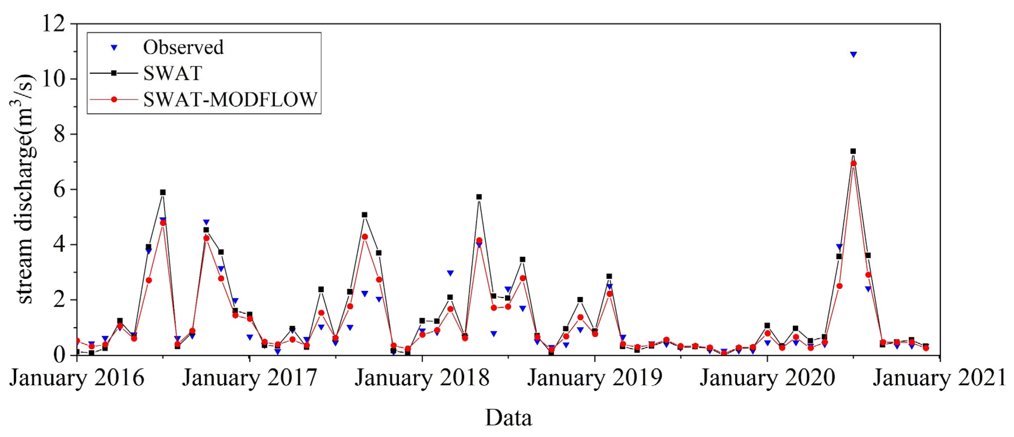
The performance of the coupled model on surface water was calibrated and validated by using the stream flow data of the Chengxi runoff hydrological station in the outlet section from 2016 to 2020. The curves of the observed and simulated values are shown in Figure 7. The stream flow fitting trend of the outlet section of the SWAT model and the SWAT-MODFLOW model is consistent with the measured flow curve. However, the SWAT model overestimates the flow at the outlet section at multiple time points during the simulation period. Moreover, the SWAT model under-simulates flood peaks. This is due to the inherent defects of the SWAT model in simulating flood prediction [28,29].

Compared with SWAT, SWAT-MODFLOW obtains more accurate results after considering the spatial distribution of the hydrogeological parameters and calculating the surface water–groundwater interactions, due to the high frequency of interaction between surface water and groundwater in the study area. The hydrographs simulated by SWAT-MODFLOW can better fit the measured values. In July 2020, the floods caused by heavy precipitation could not be simulated well by SWAT or SWAT-MODFLOW. The simulation results of SWAT and SWAT-MODFLOW are evaluated by the deterministic coefficients and Nash efficiency coefficients, and the results are shown in

Table 3. Statistical analysis between the observed and calculated monthly flows, for the SWAT and SWAT-MODFLOW models.

Name	Statistical	SWAT	SWAT-MODFLOW
Chengxi	R2	0.78	0.85
	NSE	0.76	0.83

. The deterministic coefficients and Nash efficiency coefficients of the SWAT model are 0.78 and 0.76, and the deterministic coefficients and Nash efficiency coefficients of SWAT-MODFLOW are 0.85 and 0.83.

3.2.2. SWAT-MODFLOW Performance for Groundwater

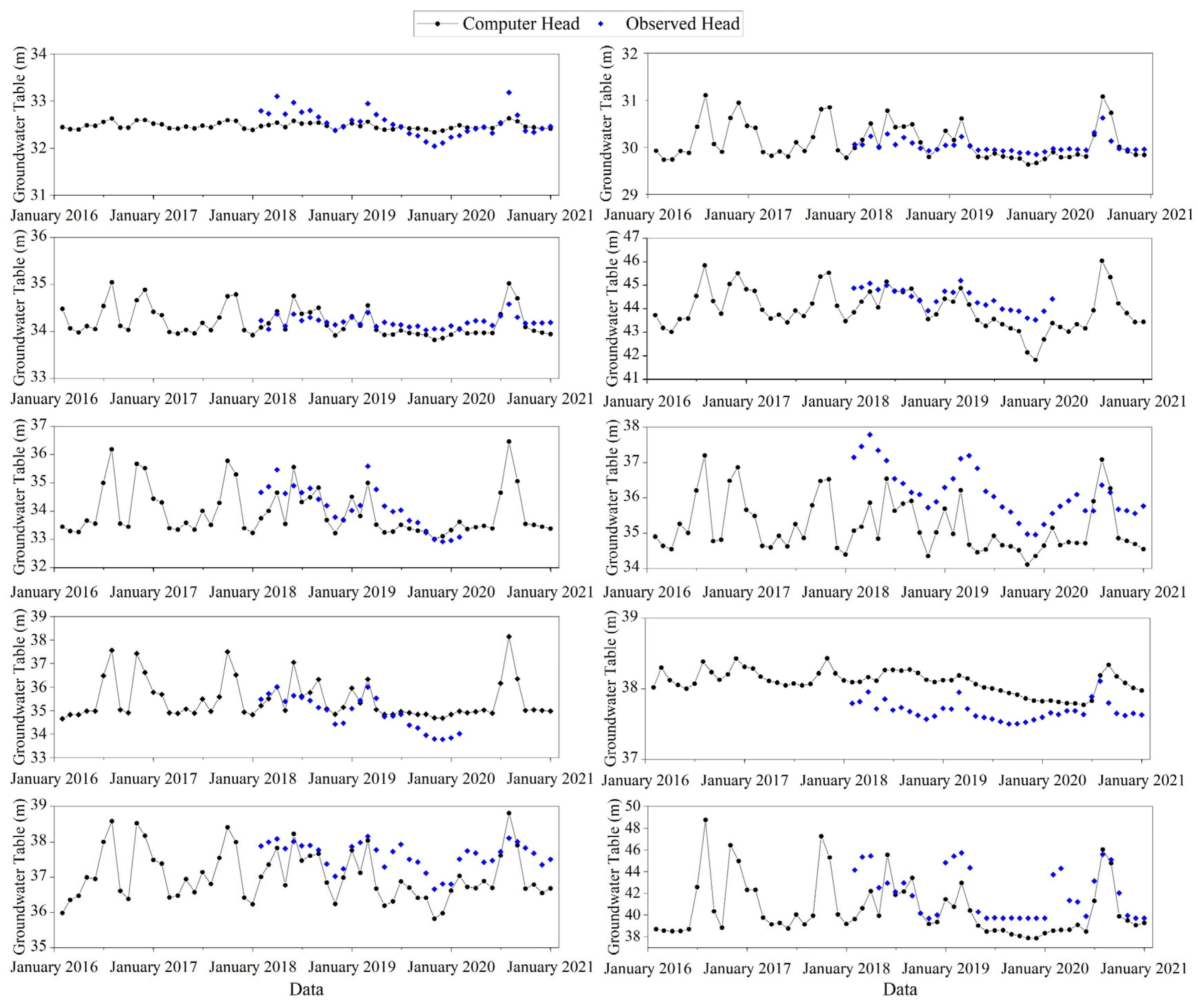
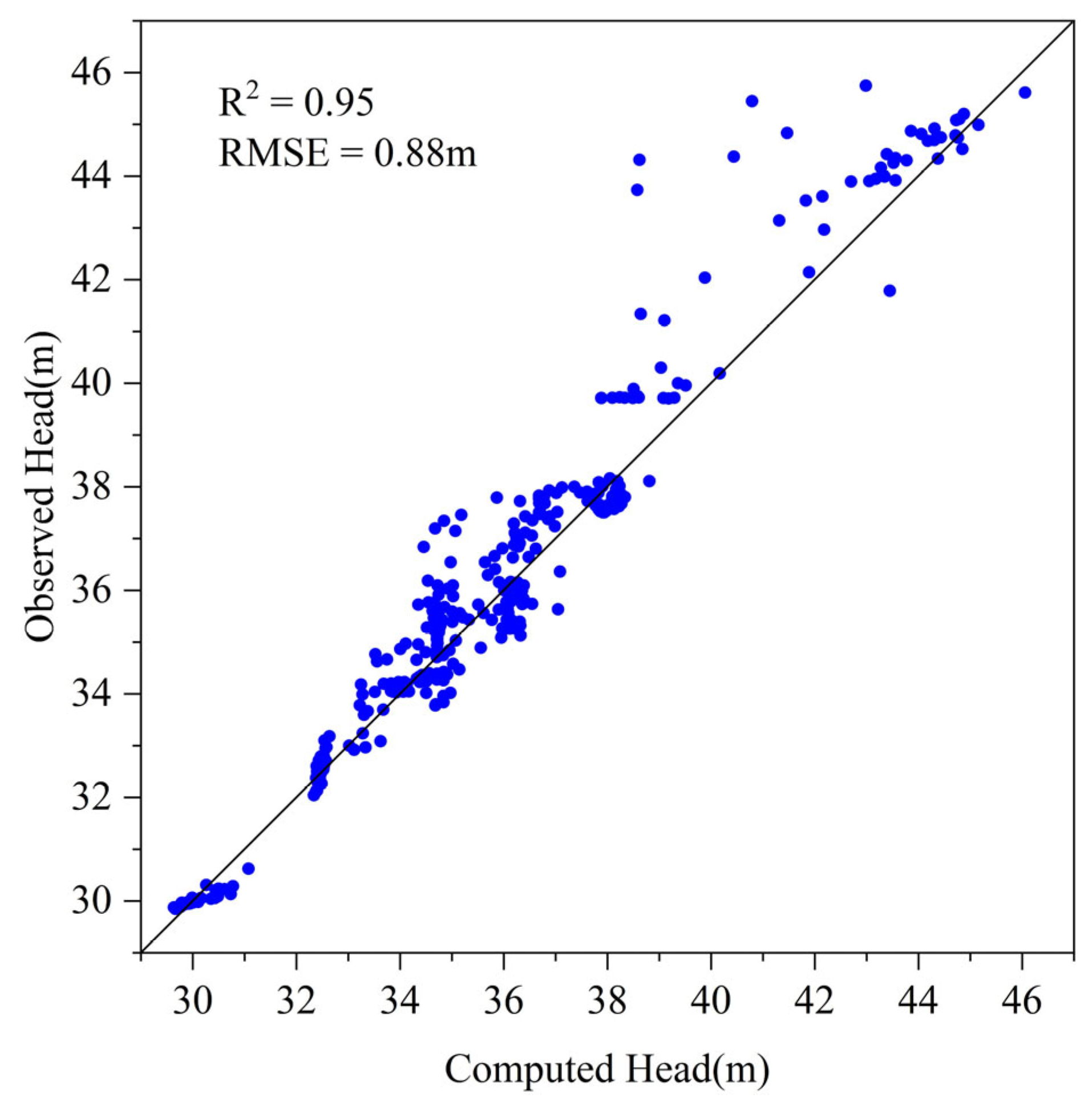
The performance of the coupled model on the groundwater was evaluated using the groundwater level of the monitoring wells from 2018 to 2020. Two indicators commonly used to evaluate groundwater models are selected: the coefficient of certainty (R²) and the root-mean-square error (RMSE). Figure 8 shows the groundwater level fitting curve of 10 monitoring wells in the study area. The SWAT-MODFLOW model can simulate the groundwater-level-variation trend of the monitoring wells. The error between the simulated value and measured value is basically controlled within 1 m. There is groundwater development and utilization in some areas of the basin, but there are no measurement data. The impact of exploitation is not considered in the numerical model. As a result, there is a gap between the simulated and measured values of the groundwater-level-changes of some monitoring wells at certain times. The scatter plots of the simulated and measured values of all monitoring wells are shown in Figure 9. The certainty coefficient (R²) of the simulated and measured values is 0.95, and the root-mean-square error (RMSE) is 0.88 m. One monitoring well was observed at a slightly higher water level than the simulated water level, because it was at the edge of a farm field. The results show that the SWAT-MODFLOW coupling model can reproduce the variation process of the groundwater level.

3.3. Spatial-Temporal Patterns of GW and SW Interaction

The annual interaction between GW and SW throughout the simulation period (2016–2020), is shown in Figure 10. Negative values represent groundwater recharge to surface water, positive values indicate that surface water recharges groundwater. During the 5-year simulation period, surface water was in a state of receiving recharge. The 5-year average groundwater recharge rate of surface water is 0.5281 m³/s, and the rate of surface water recharge to groundwater is 0.1289 m³/s. The surface–groundwater interaction varies with seasonality. The recharge of groundwater to surface water in 2019 is 0.2374 m³/s. The recharge is only 45% of the 5-year average, which is related to the precipitation of only 564 mm in 2019. The amount of groundwater-recharging surface water in 2020 is relatively lower than that in 2016–2018. Although the precipitation in 2020 is 1322 mm, following a dry year the precipitation in 2020 firstly recharged the soil moisture and aquifer.

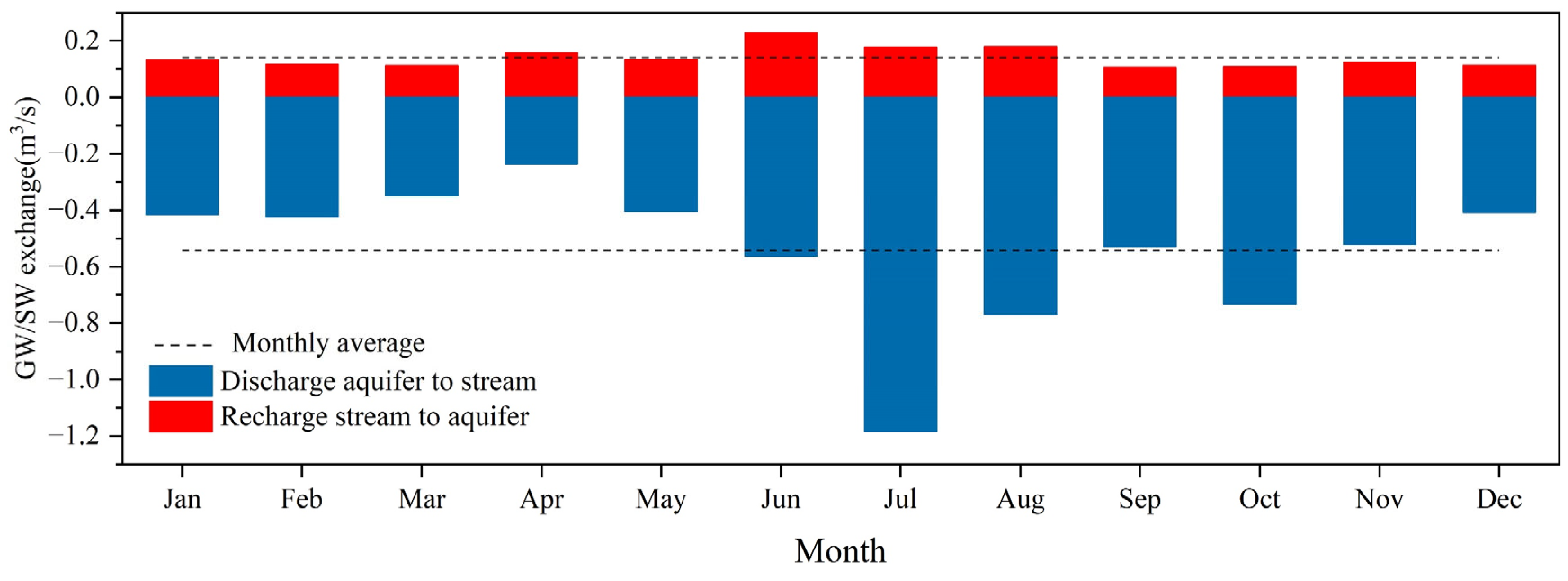
The monthly average interaction of the surface water–groundwater is shown in Figure 11. In terms of surface water recharge to groundwater, due to the heavy precipitation from June to August and the high water level of the rivers, the recharge of groundwater from the rivers accounts for 35% of the annual total recharge. From September to October, the groundwater level was already high, under the influence of previous precipitation. The reduction in precipitation resulted in lower river levels compared to previous months, with less groundwater recharge from the rivers. In terms of groundwater recharge to rivers, the recharge of groundwater to rivers is lowest in April and the highest in July. The recharge from June to August accounts for 38% of the annual recharge. In the annual dry season, the groundwater is of great significance in maintaining the natural runoff of the rivers.

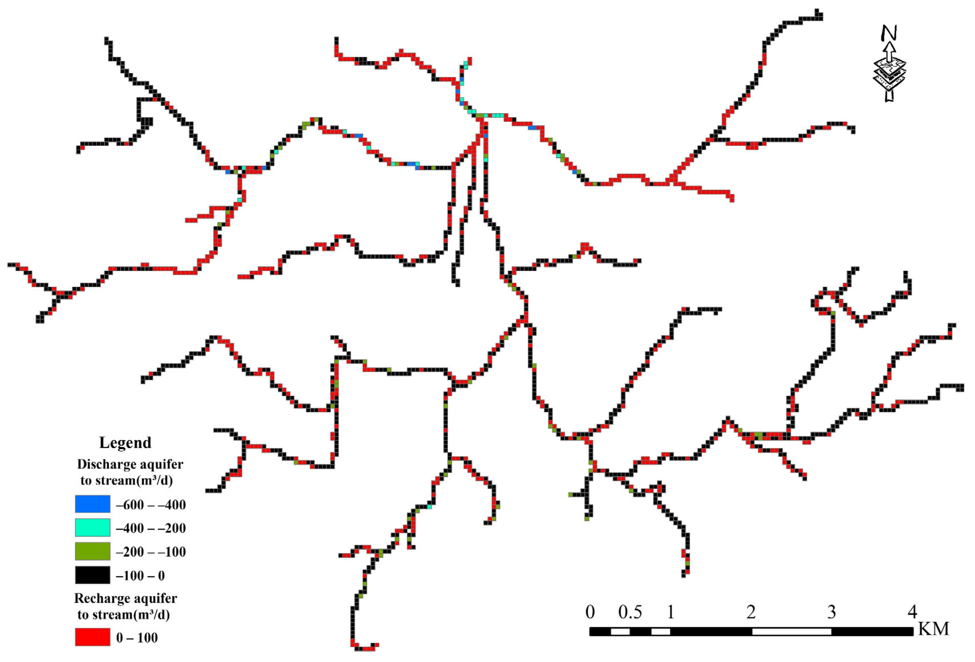
Figure 12 shows the spatial distribution of the 5-year average interaction of the surface water and groundwater for the 1836 river grids, over the entire simulation period (2016–2020). The interaction rule between the surface water and groundwater is very complex in the Huangshan basin. The amount of interaction between the surface water and groundwater in tributaries is relatively small. Whether it is the surface water recharging groundwater or the groundwater recharging the surface water, the interaction volume is mostly 0–100 m³/d. After the tributaries converge, the water level of the river rises relatively, generally manifesting as surface water supplying groundwater. It is more obvious especially near the outlet of the watershed.

Among the four sub-basins, the Zhuyuangou sub-basin is close to the outlet of the watershed, and the area is small. In general, surface water recharges groundwater, and the interaction between the surface water and groundwater is small, in the range of 0–100 m³/d. The main stream of the Dongyuan and Xiyuan sub-basins is represented as surface water supplementing groundwater; tributaries are transformed into groundwater supplementing surface water. In addition, the interaction volume of the main river is larger than that of the tributaries. Especially in the Xiyuan sub-basin, in the main stream position, the recharge of groundwater to surface water can reach 400–600 m³/d. Due to the relatively large number of human activities in the Zhongyuan sub-basin, the interaction rule between the surface water and groundwater is more complex. The surface water recharging the groundwater and the groundwater recharging the surface water alternate along the whole river. The relationship between the surface water and groundwater near the outlet of the watershed is as follows: at a distance upstream of the outlet, the surface water recharges the groundwater, and after the interaction between the Xiyuan and the Dongyuan and Zhongyuan coverage, the groundwater replenishes the surface water.

3.4. General Model Results

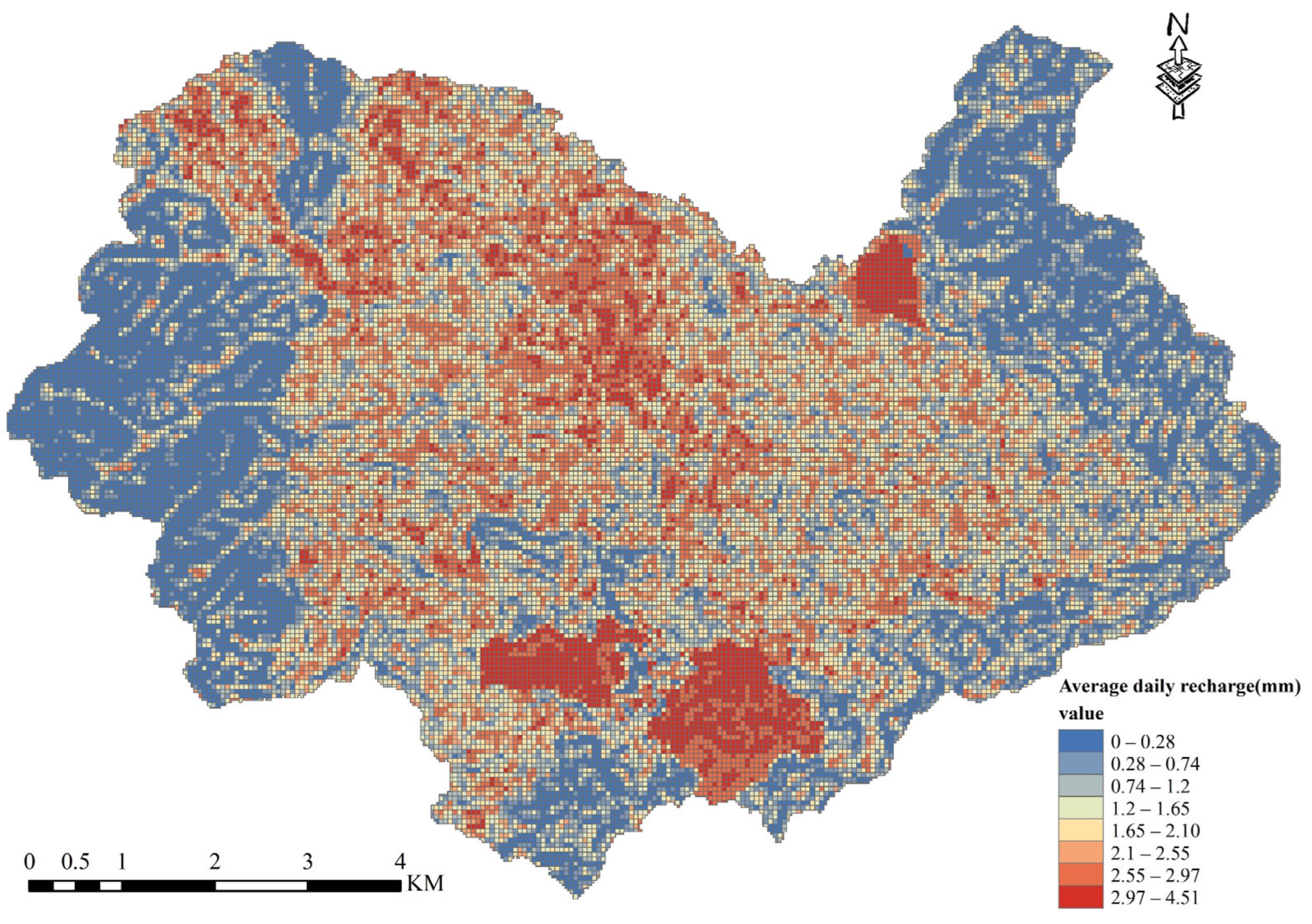
The spatial distribution of precipitation infiltration transferred from the SWAT model to the MODFLOW model on a daily average over the entire simulation period (2016–2020), is shown in Figure 13. The precipitation infiltration in the hilly area around the basin is smaller than that on the plain area. The recharge in the hilly area along the riverbed is larger than that in other surrounding hilly areas. On the plain area, the forest area is larger than other land-use types. The 5-year average infiltration coefficient of precipitation is 0.17, and the average annual infiltration coefficient of precipitation is shown in

Table 4. Annual average infiltration coefficient of precipitation.

Year	Precipitation (mm)	Precipitation Infiltration (mm)	Infiltration Coefficient of Precipitation
2016	1453.4	319.85	0.22
2017	1119.3	203.89	0.18
2018	1348.9	270.15	0.20
2019	564.1	56.7	0.10
2020	1321.6	211.69	0.16

. In 2019, the precipitation was only 564 mm, and the infiltration coefficient of precipitation was 0.1. In 2020, due to the influence of the previous dry year, precipitation had to give priority to replenishing soil moisture before recharging the saturated aquifer, so the infiltration coefficient of precipitation in 2020 is lower than that of 2016–2018. In addition, there are three areas with large precipitation infiltration spatially. The main reason is that these areas are lower in terrain than the surrounding areas, and belong to the catchment area. While the precipitation was heavy, these areas will have been submerged, and have formed a small reservoir within a certain area.

The groundwater level calculated by SWAT-MODFLOW at the end of the simulation period is shown in Figure 14. The area with the highest groundwater level appears in the hilly area around the Huashan Basin, and the area with the lowest groundwater level appears near the outlet of the entire watershed, which is consistent with the topographical conditions of the basin. In addition, because the river is recharged by groundwater, the groundwater level along the river is lower than the surrounding groundwater level. The 5-year average precipitation was slightly higher than the multi-year average. Compared with the initial groundwater level of the basin, the groundwater table at the end of the simulation period was slightly higher than the initial head.

3.5. Effect of Climate Change on Groundwater and Surface Water

3.5.1. Effects of Climate Change on Precipitation and Temperature

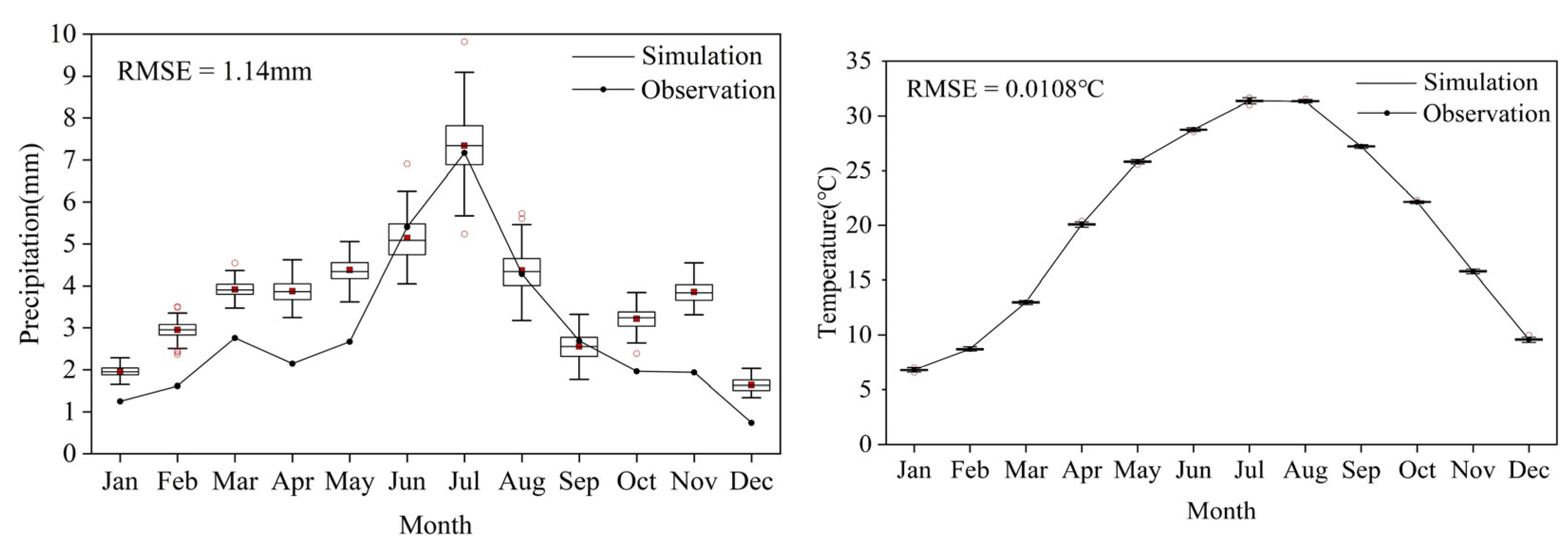
A statistical downscaling model was used to downscale the CanESM5 future climate data provided by the Canadian Climate Centre. Two scenarios, SSP2_4.5 and SSP5_8.5, were selected for the analysis of future climate change. The fitted curves for precipitation and temperature are shown in Figure 15 below, with the RMSE of 0.657 mm and 0.011 °C for the SSP2_4.5 scenario and 1.14 mm and 0.0108 °C for the SSP2_8.5 scenario. The results show that, compared with the current year, by 2050, under the SSP2_4.5 and SSP5_8.5 scenarios, the precipitation will increase by 10.32% (110.87 mm) and 13.69% (147.12 mm), respectively; the temperature will increase by 5.67% (1.15 °C) and 6.48% (1.32 °C), respectively. The historical precipitation used is 1979–2014. The historical precipitation and the precipitation results predicted by the two climate models SSP2_4.5 and SSP5_8.5, are shown in Figure 16.

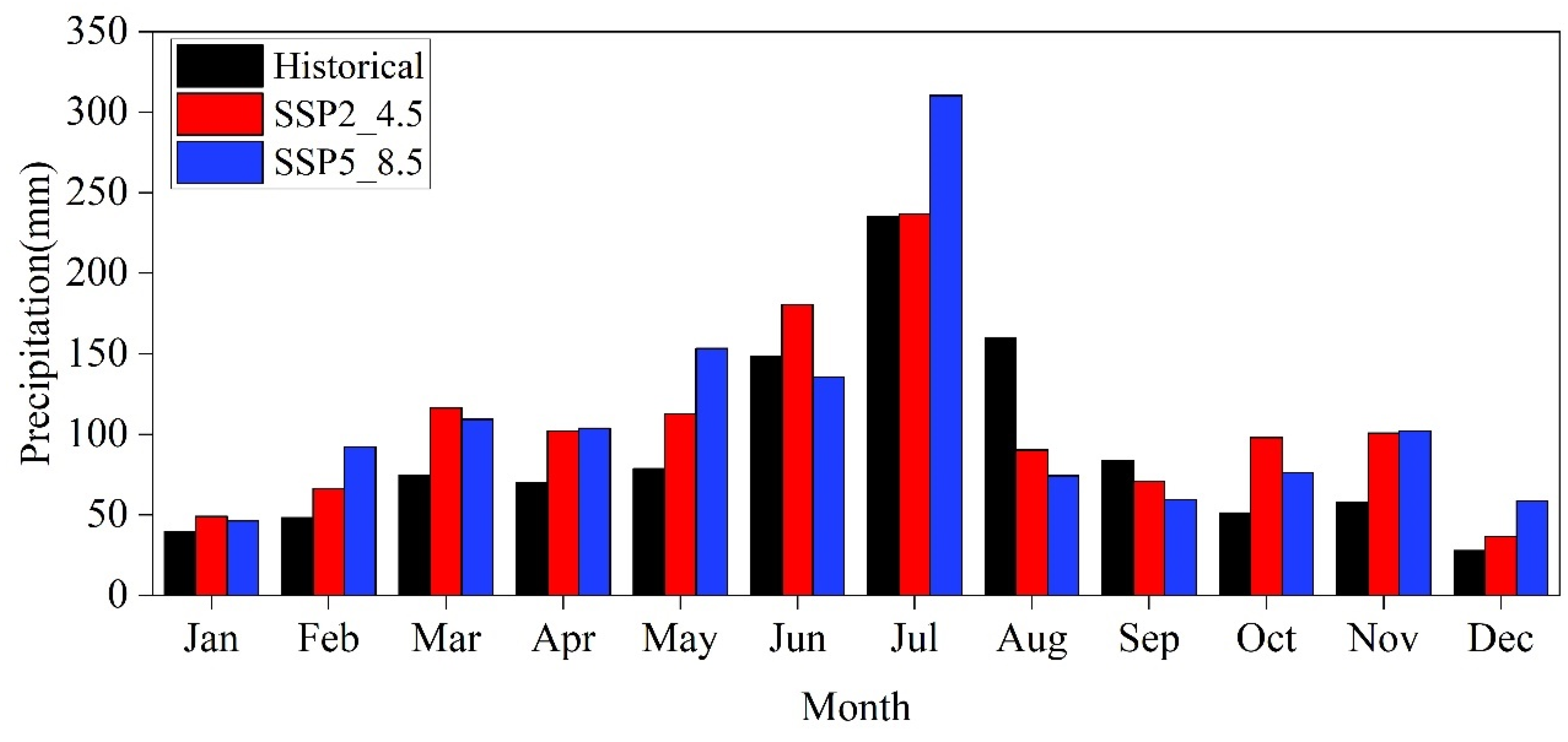
The changes in average monthly precipitation in different months of the year in historical years and under the two scenarios of SSP2-4.5 and SSP5-8.5, are shown in Figure 17. Except for August and September, the precipitation shows a downward trend, and the rest of the months show an increasing trend. The SSP5_8.5 climate scenario has more precipitation in July, and the probability of extreme precipitation is higher.

3.5.2. The Impact of Climate Change on the Spatial–Temporal Interaction between the Surface and Groundwater

In general, the occurrence of extreme weather brought about by climate change has further exacerbated the inter-annual differences in the interaction between the surface water and groundwater in the Huashan Basin. Especially in the SSP5_8.5 scenario, the minimum recharge amount of the surface water to groundwater is 0.0702 m³/s, and the maximum recharge amount is 0.1818 m³/s, a difference of 2.6 times. The maximum recharge amount of the groundwater to surface water is 1.1148 m³/s, and the minimum recharge amount is 0.1681 m³/s, a difference of 6.63 times.

Due to the increase in precipitation in the future prediction period, compared with the current (2016–2020) annual average, the ssp2_4.5 and ssp5_8.5 scenarios will both show the surface water recharge to groundwater and the groundwater recharge to surface water as an increasing trend in the next 30 years (2021–2050) (Figure 18). In the ssp2_4.5 scenario, the surface water recharges the groundwater on average 0.1583 m³/s, an increase of 22.8% compared with the base period; the groundwater recharges the surface water 0.5189 m³/s, a slight decrease compared with the base period, a decrease of 0.017%. In the ssp5_8.5 scenario, the average groundwater recharge is 0.1469 m³/s, an increase of 14.7% compared with the base period; the groundwater recharge to surface water is 0.5953 m³/s, an increase of 12.7%, compared with the base period.

The average monthly interactions of the surface water and groundwater for the two climate scenarios in the next 30 years (2021–2050) are shown in Figure 19. Compared with the base year, the recharge of the surface water to groundwater and the groundwater to surface water in August and September decreased, which was related to the decrease in precipitation in August and September during the prediction period. Due to the increasing trend of precipitation in other months, the recharging of the groundwater by the corresponding surface water also increased. In July, the SSP5_8.5 scenario had a larger discharge of the groundwater to surface water, reaching 1.2929 m³/s.

Figure 20 shows the spatial interaction pattern of the surface and groundwater for 2021–2050 in 1836 river grids of the SWAT-MODFLOW model, under the SSP2_4.5 and SSP5_8.5 scenarios. Compared with the current situation, the average surface-water– groundwater interaction in the next 30 years will be larger. It may be related to the increasing number of extreme climates. Among them, the Dongyuan sub-basin, Xiyuan sub-basin and Zhuyuangou sub-basin have obvious variation characteristics. Except for some reaches of the main stream, the interaction volume decreases, and the remaining reaches have a larger interaction volume. In addition, in the SSP2_4.5 and SSP5_8.5 scenarios, due to the increase in precipitation, the groundwater level increases. The transformation of the interaction between the surface and groundwater appears at some river segments of the tributaries. Recharged groundwater from surface water translates to surface water recharged by groundwater. Compared with the SSP2_4.5 scenario, this phenomenon is more obvious in SSP5_8.5.

It has been noted that in plain areas, where the hydraulic gradient is low, vertical upward water movement dominates. There is a strong correlation between shallow groundwater and surface water balance processes, as groundwater levels can rise to the surface with uncertain cycles [30,31]. Coupled surface groundwater models are therefore essential in analyzing surface–groundwater interactions on the plains and in the planning and management of water resources. Future changes in climate, on the other hand, can lead to changes in the groundwater head, which in turn can alter surface water–groundwater recharge and discharge relationships [32]. In this study, the SSP2_4.5 scenario resulted in 101 river cells with changing recharge and discharge relationships compared to the status quo, representing 5.5% of the entire river cells (1836). These changes in the vegetation and the benthic and nutrient relationships have a significant impact. The development of rational exploitation plans based on different water resources is essential for the sustainable development of water resources and water ecology in the basin. Climate change varies greatly among regions of the world, and requires specific analysis in the context of local conditions, and the ideas in this paper may provide a good case study for similar research.

4. Conclusions

Using the coupled numerical model SWAT-MODFLOW, the spatial–temporal interaction pattern of the surface water and groundwater in the Huashan Basin was analyzed. Compared to using one of the models alone, SWAT-MODFLOW performs better in both the stream flow and groundwater level calibration results. The applicability of SWAT-MODFLOW to small watersheds is demonstrated. By adjusting the hydraulic conductivity and specific yield of the groundwater model, the calibration of the coupled model can be validated quickly, to a certain extent.

During the simulation period (2016–2020), the spatio-temporal transformation of surface water and groundwater in the basin is complex. The average 5-year recharge rate of groundwater to surface water is 0.5281 m³/s, and the rate of surface water to groundwater is 0.1289 m³/s. The smallest excretions occur in April, and the largest excretions occur in June-September. The difference in interaction between seasons is related to the amount of precipitation. Spatially, the interaction volume of tributaries is smaller than that of the main stream, which is 0–100 m³/d. After the tributary coverage, most of them appear as surface water supplying groundwater. In addition, the interaction between surface water and groundwater at the outlet of the watershed is relatively large. The infiltration recharge in the study area is smaller in the surrounding hilly area than on the plain area. The 5-year-average-infiltration coefficient of precipitation is 0.17. The results of the prediction stage suggest that climate change scenarios are essential for the integrated management of water resources in the basin. Under the ssp5_8.5 scenario, surface water recharges to groundwater on average 0.1469 m³/s, an increase of 14.7% compared with the base period; groundwater recharges to surface water 0.5953 m³/s, an increase of 12.7% compared with the base period.

The coupled model reproduces the water cycle process in the basin, and enhances the understanding of the temporal and spatial characteristics of precipitation infiltration and surface water-–groundwater interaction. This contributes to the integrated management of water resources in the basin. After identifying the high groundwater-discharge area, the solute transport model can be further coupled in the future, to solve the current increasing problem of non-point source pollution in the watershed. In addition, the addition of isotopic data can further improve the accuracy of the coupled model.

References

1. Sophocleous, M. Interactions between groundwater and surface water: The state of the science. Hydrogeol. J. 2002, 10, 52–67. [Google Scholar] [CrossRef]
2. Kalbus, E.; Schmidt, C.; Molson, J.W.; Reinstorf, F.; Schirmer, M. Influence of aquifer and streambed heterogeneity on the distribution of groundwater discharge. Hydrol. Earth Syst. Sci. 2009, 13, 69–77. [Google Scholar] [CrossRef] [Green Version]
3. Hussein, M.; Schwartz, F.W. Modeling of flow and contaminant transport in coupled stream–aquifer systems. J. Contam. Hydrol. 2003, 65, 41–64. [Google Scholar] [CrossRef]
4. Waibel, M.S.; Gannett, M.W.; Chang, H.; Hulbe, C.L. Spatial variability of the response to climate change in regional groundwater systems—Examples from simulations in the Deschutes Basin, Oregon. J. Hydrol. Amst. 2013, 486, 187–201. [Google Scholar] [CrossRef]
5. Fleckenstein, J.H.; Krause, S.; Hannah, D.M.; Boano, F. Groundwater-surface water interactions: New methods and models to improve understanding of processes and dynamic. Adv. Water Resour. 2010, 33, 1291–1295. [Google Scholar] [CrossRef]
6. Jafari, F.; Javadi, S.; Golmohammadi, G.; Karimi, N.; Mohammadi, K. Numerical simulation of groundwater flow and aquifer-system compaction using simulation and InSAR technique: Saveh basin, Iran. Environ. Earth Sci. 2016, 75, 833. [Google Scholar] [CrossRef]
7. Priya, R.Y.; Manjula, R. A review for comparing SWAT and SWAT coupled models and its applications—ScienceDirect. Mater. Today Proc. 2021, 45, 7190–7194. [Google Scholar] [CrossRef]
8. Gumindoga, W.; Rwasoka, D.T.; Murwira, A. Simulation of streamflow using TOPMODEL in the Upper Save River catchment of Zimbabwe. Phys. Chem. Earth 2011, 36, 806–813. [Google Scholar] [CrossRef]
9. Harbaugh, A.W.; Banta, E.R.; Hill, M.C.; McDonald, M.G. MODFLOW-2000, The U.S. geological survey modular ground-water model-user guide to modularization concepts and the ground-water flow process. Open-File Rep. USA Geol. Surv. 2000, 92, 134. [Google Scholar]
10. Cornelissen, T.; Diekkrüger, B.; Bogena, H. Using HydroGeoSphere in a Forested Catchment: How does Spatial Resolution Influence the Simulation of Spatio-temporal Soil Moisture Variability? Procedia Environ. Sci. 2013, 19, 198–207. [Google Scholar] [CrossRef] [Green Version]
11. Rujner, H.; Leonhardt, G.; Marsalek, J.; Viklander, M. High-resolution modelling of the grass swale response to runoff inflows with Mike SHE. J. Hydrol. 2018, 562, 411–422. [Google Scholar] [CrossRef]
12. Gao, F.; Feng, G.; Han, M.; Dash, P.; Jenkins, J.; Liu, C. Assessment of surface water resources in the big sunflower river watershed using coupled SWAT-MODFLOW model. Water 2017, 11, 528. [Google Scholar] [CrossRef] [Green Version]
13. Bailey, R.T.; Wible, T.C.; Arabi, M.; Records, R.M.; Ditty, J. Assessing regional-scale spatio-temporal patterns of groundwater–surface water interactions using a coupled SWAT-MODFLOW model. Hydrol. Process. 2016, 30, 4420–4433. [Google Scholar] [CrossRef]
14. Yifru, B.A.; Chung, I.M.; Kim, M.G.; Chang, S.W. Assessment of Groundwater Recharge in Agro-Urban Watersheds Using Integrated SWAT-MODFLOW Model. Sustainability 2020, 12, 6593. [Google Scholar] [CrossRef]
15. IPCC. Summary for Policymakers. In Climate Change 2013: The Physical Science Basis. Contribution of Working Group I to the Fifth Assessment Report of the Intergovernmental Panel on Climate Change; Cambridge University Press: Cambridge, UK; New York, NY, USA, 2013. [Google Scholar]
16. Chu, J.T.; Xia, J.; Xu, C.-Y.; Singh, V.P. Statistical downscaling of daily mean temperature, pan evaporation and precipitation for climate change scenarios in Haihe River, China. Theor. Appl. Climatol. 2010, 99, 149–161. [Google Scholar] [CrossRef]
17. Samadi, S.; Wilson, C.A.M.E.; Moradkhani, H. Uncertainty analysis of statistical downscaling models using Hadley Centre Coupled Model. Theor. Appl. Climatol. 2013, 114, 673–690. [Google Scholar] [CrossRef]
18. Huth, R. Statistical downscaling of daily temperature in Central Europe. J. Clim. 2002, 15, 1731–1742. [Google Scholar] [CrossRef]
19. Wilby, R.; Dawson, C.; Barrow, E. SDSM-a decision support tool for the assessment of regional climate change impacts. Environ. Model. Softw. 2002, 17, 147–159. [Google Scholar] [CrossRef]
20. Hessami, M.; Gachon, P.; Ouarda, T.B.; St-Hilaire, A. Automated regression-based statistical downscaling tool. Environ. Model. Softw. 2008, 23, 813–834. [Google Scholar] [CrossRef]
21. Amin, M.Z.M.; Islam, T.; Ishak, A.M. Downscaling and projection of precipitation from general circulation model predictors in an equatorial climate region by the automated regression-based statistical. Arch. Meteorol. Geophys. Bioclimatol. Ser. B 2013, 118, 347–364. [Google Scholar] [CrossRef]
22. Wang, M.; Lu, B.; Wang, J.; Zhang, H.; Guo, L.; Lin, H. Using dual isotopes and a bayesian isotope mixing model to evaluate nitrate sources of surface water in a drinking water source watershed, East China. Water 2016, 8, 355. [Google Scholar] [CrossRef]
23. Harbaugh, A.W. MODFLOW-2005, the US Geological Survey Modular Ground-Water Model: The Ground-Water Flow Process; US Department of the Interior, US Geological Survey: Reston, VA, USA, 2005. [Google Scholar]
24. Chen, L.; Frauenfeld, O.W. Surface air temperature changes over the twentieth and twenty-first centuries in China simulated by 20 CMIP5 models. J. Clim. 2014, 27, 3920–3937. [Google Scholar] [CrossRef]
25. Hua, W.; Chen, H.; Sun, S.; Zhou, L. Assessing climatic impacts of future land use and land cover change projected with the CanESM2 model. Int. J. Climatol. 2015, 35, 3661–3675. [Google Scholar] [CrossRef]
26. Li, Y.; Yan, D.; Peng, H.; Xiao, S. Evaluation of precipitation in CMIP6 over the Yangtze River Basin. Atmos. Res. 2021, 253, 105406. [Google Scholar] [CrossRef]
27. Dai, Y.; Zhao, Y.; Lin, J.; Han, J.; Sun, X.; Li, W.; Liu, J. Analysis of slug interference tests conducted in an artificial fracture. Hydrogeol. J. 2021, 29, 895–907. [Google Scholar] [CrossRef]
28. Myers, D.T.; Ficklin, D.L.; Robeson, S.M. Incorporating rain-on-snow into the SWAT model results in more accurate simulations of hydrologic extremes. J. Hydrol. 2021, 603, 126972. [Google Scholar] [CrossRef]
29. Zakizadeh, H.; Ahmadi, H.; Zehtabian, G.; Moeini, A.; Moghaddamnia, A. A novel study of SWAT and ANN models for runoff simulation with application on dataset of metrological stations. Phys. Chem. Earth Parts A/B/C 2020, 120, 102899. [Google Scholar] [CrossRef]
30. Gu, Y.; Wang, S.; Hu, Q.; Sun, J.; Cai, M.; Lu, Z.; Gao, M. Continuous assessment of the adaptability between river network connectivity and water security in a typical highly urbanized area in eastern China. Front. Environ. Sci. 2022, 1265. [Google Scholar] [CrossRef]
31. Ochoa, C.G.; Masson, I.; Cazenave, G.; Vives, L.; Amábile, G.V. A novel approach for the integral Management of Water Extremes in plain areas. Hydrology 2019, 6, 70. [Google Scholar] [CrossRef] [Green Version]
32. Chunn, D.; Faramarzi, M.; Smerdon, B.; Alessi, D.S. Application of an integrated SWAT–MODFLOW model to evaluate potential impacts of climate change and water withdrawals on groundwater–surface water interactions in west-Central Alberta. Water 2019, 11, 110. [Google Scholar] [CrossRef]
Figure 1. Huashan Basin location in the south west of China and hydrological data stations location.
Sustainability 14 14325 g001
Figure 2. Types of land-use in the Huashan Basin.
Sustainability 14 14325 g002
Figure 3. Conceptual Model of Groundwater in Huashan Basin.
Sustainability 14 14325 g003
Figure 4. Applied simulation strategy in this research.
Sustainability 14 14325 g004
Figure 5. Measured data matched with type curves for the injecting-water type slug interference tests.
Sustainability 14 14325 g005
Figure 6. Spatial distribution of calibrated hydraulic conductivity.
Sustainability 14 14325 g006
Figure 7. Observed SWAT and SWAT-MODFLOW-simulated time series of stream discharge.
Sustainability 14 14325 g007
Figure 8. The calculated vs. observed groundwater levels over time.
Sustainability 14 14325 g008
Figure 9. Correlation of the calculated and observed groundwater levels.
Sustainability 14 14325 g009
Figure 10. 2016–2020 annual average surface water–groundwater interaction.
Sustainability 14 14325 g010
Figure 11. Monthly average of the surface water–groundwater interaction.
Sustainability 14 14325 g011
Figure 12. Annual average spatial GW–SW interaction (2016–2020). (From blue to red, the river grids for each color are 14, 20, 61, 1103 and 638 respectively).
Sustainability 14 14325 g012
Figure 13. Daily average precipitation infiltration.
Sustainability 14 14325 g013
Figure 14. Groundwater level calculated by SWAT-MODFLOW at the end of the simulation period.
Sustainability 14 14325 g014
Figure 15. Fitted curves of precipitation and maximum temperature for SSP2_4.5 and SSP5_8.5 scenarios.
Sustainability 14 14325 g015aSustainability 14 14325 g015b
Figure 16. Time series of precipitation (mm) in historical (1979–2014) and predicted (2015–2050) periods in the Huashan Basin.
Sustainability 14 14325 g016
Figure 17. Monthly average precipitation in the future under different climate scenarios.
Sustainability 14 14325 g017
Figure 18. Surface–groundwater interaction in 2021–2050 under SSP2_4.5 and SSP5_8.5 scenario. (Red represents the SSP2_4.5 scenario and blue represents the SSP5_8.5 scenario, with positive values representing surface water recharge to groundwater and negative values representing groundwater recharge to surface water.)
Sustainability 14 14325 g018
Figure 19. Average monthly GW–SW interaction in 2021–2050, under SSP5_4.5 and SSP5_8.5 scenario. (Red represents the SSP2_4.5 scenario and blue represents the SSP5_8.5 scenario, with positive values representing surface water recharge to groundwater and negative values representing groundwater recharge to surface water.)
Sustainability 14 14325 g019
Figure 20. Annual average surface water—groundwater interaction for two future scenarios.
Sustainability 14 14325 g020aSustainability 14 14325 g020b