Impacts of Land Use and Land Cover Changes on Land Surface Temperature over Cachar Region, Northeast India—A Case Study

Abstract

The promptness of industrialisation and expanding urbanisation to achieve targets of economics are resulting in the transfiguration of permeable surfaces into impervious ones through LULC adaptation, leaving a herculean footprint on the ecosystem. The LULC escalates land surface temperature (LST), which further stimulates urban heat islands (UHIs), ultimately remaining in tune with high levels of air pollution, energy use, and corresponding health hazards. The present evaluation first used Landsat TM/OLI satellite data to identify the labyrinth of the LULC rotation and, secondly, gauged its effects on the LST in the Cachar district of Assam, India, for the years 1990, 2000, 2010, and 2020. It embraces Cellular Automata (CA) and GIS methodologies to pull out the urbanization pattern and its ramifications in various LULC brackets of Cachar, India. It also embraces spatiotemporal LULC monitoring (1990–2020) and urban growth modelling (2030–2040). From the period 1990 to 2020, satellite-based LULC showed a net urban expansion of 269.43 km² (7.13% increase). Some correlations were developed to show the relationship between spatial indices such as NDVI, NDBI, and NDWI with Land Surface Temperature (LST). Resultantly, a positive relation exists between LST and NDBI, but a negative correlation prevails between LST and NDVI, as well as NDWI. This evaluation will be of service to urban and environmental planners, providing them with detailed knowledge on how land cover is changing uniquely in northeast India.

1. Introduction

Land, an indispensable element of the ecosystem, is a natural resource without which most of the habitats of organisms on earth, including human, cannot exist. Utilisation of such resource under the class of land use defines land cover as the vegetation covering a specified region. The adaptation of land use and land cover (LULC) pertains to the political, social, and economic spheres as well. Additionally, it also invests, inter alia, in the acquisition of arable land, the ecosystem, biodiversity, water bodies, the greenhouse effect, forest cover, ambient climate, and soil. The LULC is an important component of watershed features, and, in particular, it is more crucial for water resources [1]. For land resource managers, planners, and decision makers, the LULC statistics over the years, due to human-induced ecological changes such as the growth of agricultural land, the division of forests, industrialisation, and urbanisation, LULC changes have become considerable and complex in the current situation [2]. The change in the pattern of LULC in a certain area may be caused by both natural and anthropogenic influences [3]. LULC change and soil erosion in the watersheds can be reduced by vegetation cover, no-tillage practices, and increased dense forest areas. The most popular methods for surveying and tracking LULC change in any region of concern over time are GIS and satellite remote sensing (RS).

As already established, LULC alteration is mostly the result of human activity, particularly agricultural and urban expansion [4]. Due to the effects brought on by environmental, political, social, and economic factors, human influence on LULC has a dynamic and nonlinear nature [5,6]. The variation in climate, which can itself be a result of anthropogenic influences, is one of the other main causes of changes in LULC [7]. The LULC alterations are influenced by a variety of human causes, such as urbanisation and industrialisation. Despite the fact that they are important signals of development, they could harm the ecosystem [8]. Urbanisation and industrialisation alter the biodiversity, ecosystems, and geography of cities, putting pressure on the environment [9].

One of the most notable distinguishing characteristics of the current era of development is the formation of urban heat islands (UHIs), which is caused by the higher LST in any city [10]. According to a study by [11], there will be more than two billion more urban people by 2030, which will have an effect on what happens to the natural world. The LST is influenced by factors such as horizontal and vertical urbanisation, building spacing, building materials, the creation of public spaces, Micro, Small, and Medium Enterprise (MSME) centres, highways, and bus stops [12]. To comprehend the changes in LULC and their effects on the environment, numerous studies have been carried out. Regular observation and evaluation of LULC is crucial, since it has a variety of negative environmental effects that cannot be reversed [13,14]. In the course of mapping LULC changes, satellite images of different spatial, temporal, and spectral resolutions have been used [15,16]. For monitoring and forecasting LULC changes in arid and semi-arid areas, satellite images have been less used [15,17,18].

For appropriate utilisation of the natural resources within a sustainable framework, the study of LULC is obligatory. It has been observed that old or classical methods are not efficient enough to study the above-mentioned range of studies [19]. Precise and timely data of several land utilisations of an area are vital to detect deviations in the LULC [20]. Therefore, technologies such as remote sensing (RS) and Geographical Information Systems (GIS) are required to represent these data sets. However, monitoring LULC and LST depends directly on field visits, which involves a great deal of time, demands labour, and is less accurate; hence, the use of contemporary skills such as GIS and RS are effectual, with high accuracy for the extraction of the LST and identification of the LULC [21,22]. An application of statistical algorithms in remotely sensed data may extend computational power, with high-resolution satellite images also being available [23]. Models such as Multi-layer Perceptron–Markov Chain (MLP-MC), Artificial Neural Network (ANN), and Cellular Automata (CA) are implemented for a perfect simulation of undetermined LST and LULC in the municipal field of study (areas) by amalgamating RS and GIS methods [23,24]. The CA model, inter alia, is favoured over other methods because of its ability to efficiently and appropriately simulate the progression of urbanisation even at a very local scale [25].

Although much research has been conducted to examine changes in LULC, there have not been many works that directly link these traits to LST on a local level. Research at the local level, such as at district level—the smallest administrative region in India—would not only aid in the development of local land management plans, but it will also aid in the comprehension of the regional effects of climate change in the context of LULC–LST interactions. In order to determine the urbanisation pattern and its impact on various LULC classes between 2030 and 2040, the study uses built-up growth modelling (2030–2040) and spatiotemporal LULC monitoring (1990–2020) of the Cachar district. Cellular Automata (CA) and GIS approaches are also used. We use the spatial-temporal characteristics at such a fine scale to analyse LULC and LST changes over northeast India for the first time. The LULC and LST have changed significantly over the past three decades (1990–2020) in the Cachar district. The study’s primary goals are to analyse these changes and predict future changes in LULC by modelling the interaction between associated variables using the CA model in QGIS and the MOULSCE plugin and its impact on land surface temperature.

2. Study Area

Cachar district, which is located between 92°24′ E and 93°15′ E longitude and 24°22′ N to 25°8′ N latitude, is the southernmost district in the Indian state of Assam (Figure 1). The district covers a total size of 3786 km². It is bordered to the north by the Barail and Jayantia hills, to the south by Mizoram, and to the west by the districts of Hailakandi and Karimganj [26]. The main river in the area is the Barak, but it has smaller tributaries that originate in Mizoram and Manipur. A significant volume of water from the Barak River floods the entire district during the monsoon season, which lasts from April to September [27]. Most of the vegetation is of the tropical evergreen variety. In the district’s northern and southern regions, forests can be seen [28]. Several hydro-geological characteristics can be found in the district. Its annual rainfall ranges from 2000 to 2700 mm, and its temperature ranges from 12 to 34 °C, with a relative humidity of 52 to 92 percent. The majority of the study area’s landscape is flat, with a few hills scattered along the district’s perimeter. The geology of Cachar is favourable for sand, silt, clay, and gravel-based aquifers, and the majority of the aquifer layers are generally homogeneous. The district experiences a tropical climate. The population was counted as 1,736,617 people as of the 2011 census, and the population increased by 20.17 percent between 2001 and 2011. Using data from ORNL’s Landscan Population programme, the total rate of population growth from 2000 to 2020 is found to be 49% (Table 13).

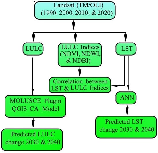
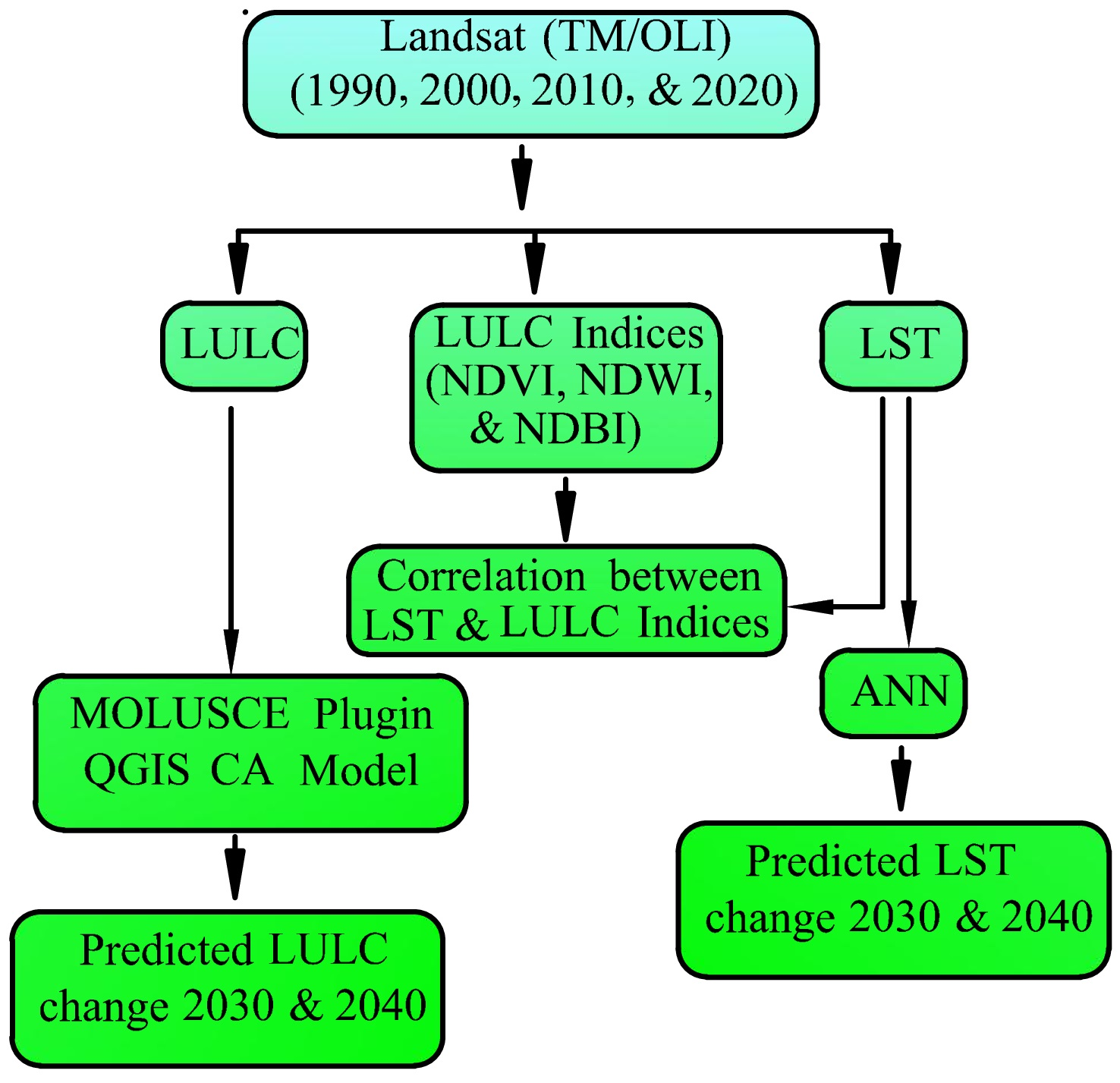
3. Materials and Methods

For the preparation of LST and LULC maps, multi-spectral Landsat TM/OLI satellite maps (1990, 2000, 2010, and 2020) were downloaded from the available website (https://earthexplorer.usgs.gov) of United States Geological Survey (USGS), with the primary aim of understanding the dynamics of built-up growth from 1990 to 2020. Several characteristics of built-up growth parameters such as Digital Elevation Model (DEM), slope, aspect, nearness to Central Business District (CBD), distance to road networks, and distance to water bodies were prepared as raster layers for modelling purposes. The change in population data were obtained from ORNL’s Landscan (https://landscan.ornl.gov/) for the years 2000, 2005, 2010, and 2020 (Figure 2).

LULC and other thematic maps were prepared using ArcGIS 8.1, whereas projection for the year 2030 and 2040 were done using the MOLUSCE plugin in QGIS 3.1, as shown in (Figure 3).

3.1. Classification of LULC Classes and Accuracy Assessment

As the Landsat satellite images are already corrected in geometric and radiometric alterations, there was no additional requirement of image-to-image geo-registration or image-to-image rectification. The threshold value for the maximum overcast was fixed at 5% during the image downloading process to obtain images with very little cloud cover or cloud-free images. Based on the availability of satellite images, the images were downloaded with a time difference of 10 years from 1990 to 2020. To maintain integrity, all the Landsat images of the same or near dates were utilised, i.e., months of December/January [29,30]. Using suitable combinations of bands, we generated true colour composites (TCCs) for each year’s images to train samples for five different land use classes (dense water bodies, agricultural land, vegetation, built-up, and others) for the mentioned years using the Maximum Likelihood Supervised Classification (MLSC) technique [31].

Table 1. Description of Landsat and DEM data used.

Data	Year	Acquired Date	Path/Row	Multi-Spectral Band Resolution
LANDSAT 5 TM	1990	16 January 1990	136/43	30 m
LANDSAT 5 TM	2000	13 February 2000	136/43	30 m
LANDSAT 7 ETM+	2010	12 February 2010	136/43	30 m
LANDSAT 8 OLI	2020	19 January 2020	136/43	30 m
Digital elevation model, Cartosat I-V3				30 m

and

Table 2. Description of land use and land cover types.

Land Cover Types	Description
Dense Vegetation	Forest, stunted trees, or bushes
Agricultural Land	Grassland, park, fallow land, playground, and cropland
Water bodies	River, lakes, reservoirs, ponds, and wetlands
Built-up	Commercial, residential, industrial building, road
Others	Bare soils, open space, vacant land, sand, and landfill sites

gives a brief description of satellite images used in this study and major LULC classes.

The primary focus of this study is to simulate the built-up class, which includes residential areas, institutions, commercial complexes, etc. The green cover is classified into two categories: dense vegetation and agricultural land. The water bodies class includes rivers, canals, ponds, etc., and the rest of the land was classified as the other class, which is composed of bare land, wastelands, rock outcrops, etc. The accuracy assessment of LULC maps was done using ground truths from attainable Google Earth images. One of the most vital steps in the classification of Landsat images into various classes is referred to as the “accuracy assessment”. The purpose of the accuracy assessment is to determine how well the pixels in Landsat images are classified into the appropriate LULC classes in a quantitative manner. For the purpose of determining the degree to which the classified images are accurate, the error matrix and the Kappa coefficient are both put to use [32]. An error matrix is constructed by comparing the error values for each LULC category with their respective ground truth values. This comparison is done so that the precision of the classification can be assessed. This is done so that the error matrix may be prepared properly [33]. The number of classes is proportional to the number of rows and columns in the error matrix, which both have the same total number. The rows of the table represent the ground truth image, whereas the columns contain the same classes and represent the categorised image (Wilkie & Finn, 1996) [34]. The Kappa coefficient can be used to assess the degree to which the error matrix is consistent as a whole. The Kappa coefficient, denoted by $K^{^}$, can be calculated with the help of Equation (1):

$$K^{^}=\frac{n{{\displaystyle \sum }}_{i=1}^k{n}_{ii}-{{\displaystyle \sum }}_{i=1}^k{n}_{i+}{n}_{+i}}{n^2-{{\displaystyle \sum }}_{i=1}^k{n}_{i+}{n}_{+i}}$$

(1)

where

$$\begin{gathered} k=\mathrm{No}. \mathrm{of}\frac{\mathrm{rows}}{\mathrm{columns}}\mathrm{in} \mathrm{the} \mathrm{error} \mathrm{matrix}, \mathrm{n}=\mathrm{No}. \mathrm{of} \mathrm{observations} \mathrm{in} \mathrm{the} \mathrm{error} \mathrm{matrix}, n_{ii}= \\ \mathrm{Diagonal} \mathrm{component} \mathrm{in} \mathrm{row} \mathrm{i} \mathrm{and} \mathrm{column} \mathrm{i}, n_{+i}=\mathrm{No}. \mathrm{of} \mathrm{observations} \mathrm{in} \mathrm{column} \mathrm{i} \end{gathered}$$

Classification accuracy is the percentage of samples correctly classified in an error matrix. To assess classification/overall accuracy, divide the total number of correctly categorised samples by the total number of reference samples using Equation (2).

$$Overall accuracy=\frac{Total no.of samples taken for classes that are classified correctly}{Total no.of reference samples taken for classification}$$

(2)

In order to calculate the mapping accuracy of LULC classes, both producer and user accuracy are calculated using Equations (3) and (4)

$$Produce{r}^{\prime }s Accuracy=\frac{a_{ii}}{{{\displaystyle \sum }}_{i-1}^n{a}_{i+}}$$

(3)

where$a_{ii}$ = No. of samples correctly classified, $a_{i+}$ = Column total for class i, and $a_{+i}$ = Row total for class i.

$$Use{r}^{\prime }s Accuracy=\frac{a_{ii}}{{{\displaystyle \sum }}_{i-1}^n{a}_{i+}}$$

(4)

Final prepared LULC maps were used in the analysis of built-up growth and land use/land cover change dynamics during 1990–2020 and also for calibrating the model. Major road networks and water bodies are important factors for the built-up growth and were obtained by digitising the recent LANDSAT images (2020). With the help of a digitised shapefile, we generated the raster that represents nearness to the major road network and nearness to major water bodies which are further classified at an interval of 1 km each. Similarly, for CBD location, which was considered as Silchar, we prepared a multi-ring buffer around Silchar in an interval of 3 km in 18 classes from high nearness to low nearness. Then we rasterised the vector layers at 30 m pixel size and extracted a constant level to tie the projection, cell size, and geometry of the previous layers. To prepare the slope and aspect maps, we used Cartosat–I, V3 DEM data of 30 m spatial resolution, taken from Indian earth satellite data site BHUVAN (http://bhuvan.nrsc.gov.in).

3.2. Estimation of LST

We used thermal bands of Landsat to calculate LST for the years 1990, 2000, 2010, and 2020. A four-step process to calculate LST from Landsat 5 TM (for the years 1990 and 2000), and six-step procedure for Landsat 8 OLI images (for the years 2010 and 2020) were utilised. The first step is to convert the DN value of the TIR band into spectral radiance ($L_{\lambda }$) using Equation (5) [35].

$$L_{\lambda }=\left(\frac{L_{MAX}-L_{MIN}}{Q_{CALMAX}-Q_{CALMIN}}\right)\ast DN-1+L_{MIN}$$

(5)

$L_{MAX}=$ SR that is scaled to $Q_{CALMAX}$ in $\mathrm{W}/ \left({\mathrm{m}}^2 \ast \mathrm{sr} \ast \mathsf{\mu }\mathrm{m}\right)$

$L_{MIN}=$ SR that is scaled to $Q_{CALMIN}$ in $\mathrm{W}/ \left({\mathrm{m}}^2 \ast \mathrm{sr} \ast \mathsf{\mu }\mathrm{m}\right)$

$Q_{CALMAX}=$ maximum quantised calibrated pixel value (corresponding to $L_{MAX}$) in $DN=255$

$Q_{CALMIN}=$ minimum quantised calibrated pixel value (corresponding to $L_{MIN}$) in $DN=1$

$DN$ is the thermal band for Landsat 5

$L_{MAX}$and $L_{MIN}$ are taken from the metadata file given with the image

Plank’s inverse function is used in the calculation of effective brightness temperature (TB) at-sensor, which is also known as black body temperature, using Equation (6).

$$T_B=\frac{K_2}{L_{n }\left(\frac{K_1}{L_{\lambda }}+1\right) }$$

(6)

where $K_2$ (constant) = 1260.56 K and $K_1$ = 607.66 ($\mathrm{mW} \times {\mathrm{cm}}^{-2}\times { \mathrm{sr}}^{-1}$) for Landsat 5.

The concluding Land Surface Temperature (LST) is calculated using Equations (7) and (8).

$$LST=\frac{T_B}{\left(\lambda +\raisebox{1ex}{$T_B$}\!\left/ \!\raisebox{-1ex}{$\rho $}\right.\right)\ast L_n\epsilon +1}$$

(7)

where $\lambda$ is the wavelength of emitted radiance, equal to $11.5 \mu \mathrm{m}$

$$\rho =h.c/\sigma$$

(8)

$\sigma =$ Stefan Boltzmann’s constant ($5.67\times {10}^{-8}{ \mathrm{Wm}}^{-}{}^2{\mathrm{K}}^{-}{}^4$)

$h=$ Plank’s constant ($6.626\times {10}^{-}{}^{34} \mathrm{J}$ s)

$c=$$2.998\times {10}^8 \mathrm{m}/\mathrm{s}$, which is speed of light

$\epsilon =$ spectral emissivity.

The value of the spectral emissivity coefficient is taken as unity in this study.

The calculated LST, which is in kelvin, was converted into Celsius using Equation (9)

$$LS{T}_c=LST-273.15$$

(9)

To derive the LST using Landsat 8 OLI thermal bands, we followed these seven steps.

Step 1: We used Landsat 8 bands 2–5 and band 10 (TIRS) for the calculation of spectral radiance (SR) using Equation (10).

$$L=\left(\frac{L_{max}-L_{min}}{D{N}_{max}}\right)\times Band+L_{min}$$

(10)

where

$L=$ Atmospheric SR in $\raisebox{1ex}{$\mathrm{watts}$}\!\left/ \!\raisebox{-1ex}{$\left({\mathrm{m}}^2\times \mathrm{srad} \times \mathsf{\mu }\mathrm{m} \right) $}\right.$

$L_{max}=$ Maximum SR of respective bands

$Band{L}_{min}=$ Minimum SR of respective Bands

$D{N}_{max }=Q_{cal max}$ – $Q_{cal min}$ is the difference between the minimum and maximum sensor’s calibration.

Step 2: We converted the data of the TIRS band from SR to BT with the help of thermal constants given in the metadata file using Equation (11).

$$BT=\frac{K_2}{Ln \left( \frac{K1 }{L_{\lambda }}+1 \right)}-273.15$$

(11)

where $K_2$ and $K_1$ are band-specific constants and, for Landsat 8 OLI, values of $K_2$ are 1201.1442 and 1321.0789 for band 11 and 10, respectively, and $K_1$ values for band 10 and 11 are 774.8853 and 480.8883, respectively.

$BT=$ Brightness temperature (Celsius).

Step 3: Then we calculated NDVI with the help of NIR band and Red band using Equation (12) [36].

$$NDVI=\left(\frac{NIR band-Red band }{NIR band+Red band }\right)$$

(12)

where range of NDVI is $-1 to+1$. Values ranging from 0 to +1 indicate vegetation cover, while values close to 1 indicate dense vegetation.

Step 4: with the help of the highest and lowest value of NDVI, $P_v$ (Proportion of Vegetation) was calculated and used in Equation (13) [37].

$$P_v={\left(\frac{NDVI-NDV{I}_{min}}{NDV{I}_{max}-NDV{I}_{min}} \right)}^2$$

(13)

Step 5: Then we calculated LSE (Land Surface Emissivity) with the help of $P_v$, calculated above, using Equation (14) [38].

$$LSE=0.004 x P_v+0.986$$

(14)

Step 6: We used Equations (15) and (16) to calculate LST in degrees Celsius.

$$LST=\frac{BT}{\{ 1+\left[\frac{\lambda BT}{\rho }\right]\ln \left(LSE\right)\}}$$

(15)

where $\rho$ was calculated using the Equation (16):

$$\rho =h \frac{c}{\sigma }=1.438\times {10}^{-2}mk$$

(16)

where $\sigma$ is Boltzmann constant ($1.38\times {10}^{-23} \mathrm{J}/ \mathrm{K}$), h is Planck’s constant ($6.626\times {10}^{-34} \mathrm{J} \mathrm{s}$), and $c$ is the velocity of light ($2.998\times {10}^8 \mathrm{m}/\mathrm{s}$).

3.3. Cellular Automata

It is a discrete mathematical model of an infinite, regular lattice in a finite number of dimensions, which consists of cells, in this case the raster, each in a finite number of states [39]. Here, attributes of each cell are determined by a set of transition rules [40]. This formulates a CA model script, considering all factors which contribute to built-up growth within the study area. A kernel of (3 × 3) size held the test pixel at its centre, as shown in Equation (17).

$$A_{i,j}^t=\left[\begin{array}{ccc}{a}_{i-1, j-1}^{\left(t\right)}& a_{i-1, j}^{\left(t\right)}& a_{i-1, j+1}^{\left(t\right)}\\ a_{i,j-1}^{\left(t\right)}& a_{i,j}^{\left(t\right)}& a_{i,j+1}^{\left(t\right)}\\ a_{i+1 ,j-1}^{\left(t\right)}& a_{i+1, j}^{\left(t\right)}& a_{i+1, j+1}^{\left(t\right)}\end{array}\right] 3\times 3 neighbourhood$$

(17)

The model primarily depends on a set of transition rules such as present state of immediate neighbouring pixels and present state of testing pixels. It examines the dependency of the present and future (t + 1) state of pixels on the set of transition rules $\left(\varnothing \right)$ as per Equation (18) [41]:

$$a_{i,j}^{t+1}=\varphi \left(A_{i,j}^t\right)$$

(18)

The transition rules $\left(\varphi \right)$ are the function of conditional statements with different threshold values, which can be represented as Equations (19)–(21):

$$\varphi =f \left(T, B\right)$$

(19)

$$T=\left\{TR, TW, TC, TS, TA\right\}$$

(20)

$$B=\left\{BR, BW, BC, BS, BA\right\}$$

(21)

where TR, TW, TC, TS, and TA are the threshold values of nearness to road, nearness to water bodies, nearness to CBD, slope, and aspect, respectively, whereas BR, BW, BC, BS, and BA are the respective built-up pixels in the kernel for every element that belongs to threshold T. The DEM, Slope, Aspect, CBD, nearness to road, and nearness to water bodies are shown in (Figure 4).

We initiated the model calibration part with the help of previously prepared LULC for the year 1990 and 2000 to predict the LULC of 2010; similarly, we used LULC of 2000 and 2010 to simulate for 2020, LULC of 2010 and 2020 to simulate for 2030 LULC, and LULC of 2020 and simulated 2030 to predict LULC of 2040 [42]. We validated the simulated LULC of the years 2010 and 2020 using the prepared satellite-based LULC of 2010 and 2020. For this we used the MOLUSCE plugin of QGIS software 3.1 only by calculating the percentage of correctness between these years.

3.4. Calculation of NDWI and NDBI

In order to characterise the land cover class that was related to LST, NDBI, NDVI, and NDWI were used. In prior research, NDVI was utilised for the monitoring drought, agricultural production, and the density of vegetation [43,44,45,46]. The NDVI was computed by making use of the following Equation (12). The NDBI can be used as an indication of the built-up area because of its sensitivity to urban environments. The NDWI is utilised for the purpose of monitoring the water content of vegetation and calculated using Equation (23) [47,48]. One of the most important categories of land cover is represented by the normalised difference build-up index (NDBI), which measures built-up areas calculated using Equation (23) [49]. In order to explore the connection between LST and various land cover indices, the method of randomly selecting points and applying it was used [22,45,50], and the coefficient of determination $R^2$was calculated.

$$NDBI=\left(\frac{SWIR 1-NIR}{SWIR 1+NIR}\right)$$

(22)

$$NDWI=\left(\frac{NIR-SWIR 1}{NIR-SWIR 1}\right)$$

(23)

where NIR stands for Near Infrared and SWIR stands for Shortwave Infrared. For Landsat 5 TM, NIR is band 4 and SWIR1 is band 5, whereas for Landsat 8 OLI, NIR is band 5 and SWIR1 is band 6.

3.5. Land Surface Temperature Simulation

As an important part of the study, simulations were used to predict the temperature for the next two decades. There are many ways to predict simulated temperature, such as the MOLUSCE tool in QGIS, Artificial Neural Networks, hybrid neural models, Markov chain, regression models, etc. [51]. We simulated the LST for the years 2030 and 2040 using an ANN tool. The sample point for the ANN model was generated by dividing the research region into 300 m × 300 m spatial grids in QGIS. This grid size was determined by calculating the smallest area over which a single feature might significantly alter the LST [9]. In order to develop the prediction model, we used the land use land cover (LULC), normalised differential vegetation index (NDVI), normalised differential built-up index (NDBI), and land surface temperature (LST) of the years 1990, 2000, and 2010 as input parameters and LST for the year 2020 as target data and predicted the 2020 LST (Figure 5) [9,22,43]. We used the feed-forward backprop method as a network type, with a total of 10 neurons, and PURELIN as a transfer function to run the ANN model in MATLAB. Correlation coefficients $\left(R\right)$ were used to evaluate the accuracy of the model using Equation (24). We trained the model with accuracy for training: $R$= 0.775, Validation: $R$= 0.778, Test: $R$= 0.780 and AII: $R$= 0.776 (Figure 6). To simulate the LST for the years 2030 and 2040, we used the NDVI, NDWI, NDBI, and LST at an interval of 10 and 20 years and supplied them to the above trained model [52,53]. The final $R$ value ranges between 0.5 to 0.7, which shows strong positive correlation [54,55]. Pixel value data of the image were changed to discrete (point) data values using ArcGIS Version-10.6.1.

$$R=\frac{\sum \left(T_{obs}-\overline{T_{obs}}\right)\left(T_{model}-\overline{T_{model}}\right)}{\sqrt{\sum {\left(T_{obs}-\overline{T_{obs}}\right)}^2\sum {\left(T_{model}-\overline{T_{model}}\right)}^2}}$$

(24)

4. Results

We prepared and analysed the satellite-based LULC maps in the study area, during 1990–2020. As discussed above, the spatio-temporal distribution and prediction of future LULC and LST were also done. The following sections describe the results.

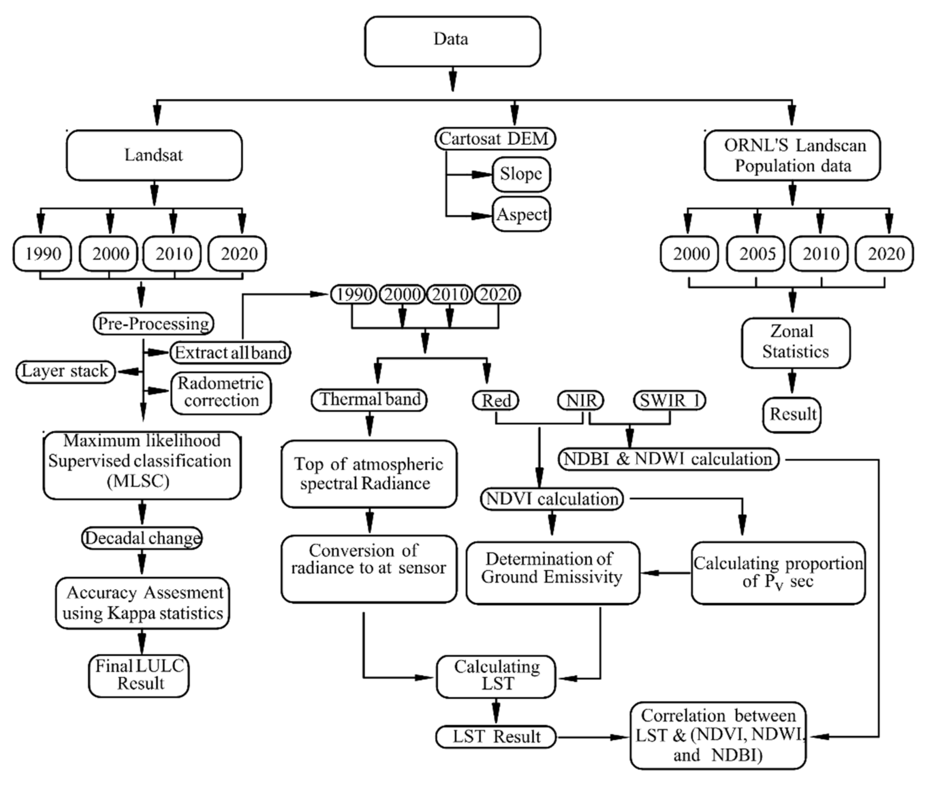
4.1. Analysis of LULC Change

In this segment, we discuss the changes that have taken place in the LULC over three decades (1990–2020). The further discussion also describes the growth pattern of built-up regions and decadal land cover transition from 1990 to 2000, 2000 to 2010, 2010 to 2020, and 1990 to 2020.

LULC Mapping and Accuracy Assessment

We applied the Maximum Likelihood Supervised Classification (MLSC) method in different Landsat images (TM/OLI) to analyse the variations and change patterns of LULC (1990–2020) (Figure 7). Change trends can be clearly observed in Figure 8; for example, built-up land increases gradually, with a decrease in dense vegetation and agricultural land areas over the entire study period. This preliminary analysis suggested that there is a direct influence of urban growth on the natural environment. After the analysis and proper observation of the results, it is seen that there has been an increase in built-up areas and the formation of new water bodies in the places where earlier dense vegetation and agricultural land existed. The analysis depicts the encroachment of human needs on the natural ecosystem. The statistics of the real LULC are shown in (

Table 3. Area statistics of the actual land use land cover for the year 1990, 2000, 2010 and 2020.

LULC Class	1990		2000		2010		2020
	Area in km2	Area in %	Area in km2	Area in %	Area in km2	Area in %	Area in km2	Area in %
Dense Vegetation	2302.84	60.92	2297.40	60.78	2262.42	59.85	2134.09	56.46
Agricultural Land	1133.64	29.99	1025.43	27.13	981.80	25.97	943.07	24.95
Water bodies	131.19	3.47	128.06	3.39	156.72	4.15	232.78	6.16
Settlement	196.63	5.20	314.28	8.31	374.62	9.91	466.05	12.33
Others	15.73	0.42	14.86	0.39	4.47	0.12	4.04	0.11

).

Table 4. Accuracy assessment of Landover classified maps for the years 1990, 2000, 2010, and 2020.

User’s Accuracy						Producer’s Accuracy					Overall Accuracy
Year	Dense Vegetation	Agricultural Land	Water Bodies	Built-Up	Others	Dense Vegetation	Agricultural Land	Water Bodies	Built-Up	Others
1990	100	97.67	97.43	96.87	90.91	97.37	100	100	86.11	100	96.74
2000	97.5	95	97.3	97.5	100	97.5	100	97.3	95.12	95.83	97.22
2010	100	92.86	90.91	90.48	100	97.62	94.55	90.91	92.68	94.74	94.21
2020	97.77	97.5	97.22	97.29	100	95.62	100	100	94.73	100	97.9

shows the results of the overall accuracy assessment, which is 96.74%, 97.22%, 94.21%, and 97.9% in 1990, 2000, 2010, and 2020, respectively. The Kappa statistic is an evaluation of accuracy that takes into account all variables but does not take into account the effect of random variation on accuracy [56]. The Kappa ($K^{^}$) statistics are used to evaluate the overall accuracy of the LULC classes because they offer a statistically valid evaluation of the quality of categorisation. This evaluation is carried out by applying the Kappa statistics. When the $K^{^}$ value is more than 0.5, the modelling of LULC change is considered to be good, according to [57]. During this same time period, [58] believed that the performance of the classification was outstanding if $K^{^}$ was greater than 0.79, substantial if 0.6 $K^{^}$ was less than 0.79, and in moderate or poor agreement if $K^{^}$ was less than 0.59. An error matrix can be used to determine the percentage of samples that were correctly classified, which can be used to determine the overall accuracy of the classification. It is possible to compute it by dividing the total number of samples that were successfully classified by the total number of samples that were used as references for the classification [59].

4.2. Land Cover Transition Assessment

The investigation of LULC changes is important for simulating the future LULC [22]. It is observed that the built-up growth has been significant in the Silchar city. This is also in accordance with the findings in the paper. Figure 9 illustrates the contribution of net transition from different land cover to the built-up area.

Table 5. Decadal Change in LULC change.

LULC Class	1990–2000		2000–2010		2010–2020		1990–2020
	ΔArea (Km2)	Δ%	ΔArea (Km2)	Δ%	ΔArea (Km2)	Δ%	ΔArea (Km2)	Δ%
Dense Vegetation	−5.45	−0.14	−34.97	−0.93	−128.33	−128.33	−168.75	−4.46
Agricultural Land	−108.21	−2.86	−43.63	−1.15	−38.73	−38.73	−190.57	−5.04
Water bodies	−3.13	−0.08	28.66	0.76	76.06	76.06	101.59	2.69
Settlement	117.65	3.11	60.34	1.60	91.44	91.44	269.43	7.13
Others	−0.87	−0.02	−10.39	−0.27	−0.43	−0.43	−11.69	−0.31

shows the decadal changes in LULC during 1990–2000, 2000–2010, 2010–2020, and 1990–2020. From this table, we can say that the authentic built-up area growth, which was 196.63 km² (about 5.2% of total area) in 1990, was extended to 314.28 km² (8.31% of total area) in 2000, 374.62 km² (9.9% of total area) in 2010, and 466 km² in 2020 (12.32 % of total area). It is understandable that the role of human influence has caused the change in LULC dynamics. A decrease in dense vegetation and agricultural land cover can be seen by 60.92% and 29.99% in 1990 to 56.46% and 24.95% in 2020, respectively. Similarly, an increase in water bodies can be observed by about 3.47% in 1990 to 6.16% in 2020. The overall change (from 1990 to 2020) in the water bodies was observed as +2.96%, as overall water body coverage in 1990 was 131.19 km², which was increased to 232.78 km² in 2020. There is also a change in the other classes for the same period, which is measured as 0.42% (15.73 km²) to 0.11% (4.04 km²). This shows how the direct influence on different LULC classes became visible in rapid built-up area growth during 1990–2020. Table 5 shows that, in the past 30 years, the area of built-up land and water bodies has increased by 7.13% and 2.69%, respectively. Similarly, a net loss of dense vegetation and agricultural land is 168.75 Km² (4.46%) and 190.57 Km² (5.04%) of their area, respectively. The decline in land classified as “Others” (0.31%) was transferred to built-up areas and water bodies gradually during 1990–2020. These changes may have contributed to an increase in the built-up area due to economic development and commercial activities in the study region.

From the analysis, we found that there are gains, as well as losses, experienced by all the classes in respective years. Agricultural land, dense vegetation, and land classified as “Others” faced a significant amount of loss from 1990 to 2020. In the past three decades, a significant gain in the built-up area (7.13%) and water bodies (2.69%) can be seen. The net increase in the built-up areas was 3.1% (1990–2000), 1.59% (2000–2010), and 2.42% (2010–2020) (Figure 10).

LST Change Analysis

The spatial and temporal distribution of LST was determined using the Landsat 5 TM and Landsat 8 OLI thermal bands for the entirety of the study years (1990–2020). Based on the lower and higher LST values that were recovered from different years, the LST values were divided into five ranges (≤20, 20–25, 25–30, 20–35, and 35 °C), and the proportion of areas that fell within each range was computed (Figure 11). According to

Table 6. Area statistics of the actual land surface temperature for the years 1990, 2000, 2010, and 2020.

LST in (°C)	1990		2000		2010		2020
	Area in km2	Area in %	Area in km2	Area in %	Area in km2	Area in %	Area in km2	Area in %
≤20	750.43	19.85	629.60	16.66	361.19	9.56	240.48	6.36
20–25	984.82	26.05	607.75	16.08	779.25	20.61	923.32	24.43
25–30	815.39	21.57	894.48	23.66	875.17	23.15	841.16	22.25
30–35	715.06	18.92	969.28	25.64	1019.34	26.97	1014.31	26.83
≥35	514.34	13.61	678.91	17.96	745.07	19.71	760.77	20.13

, in 1990, approximately 19.85% (750.43 km²) and 26.05% (984.82 km²) of the area fell within the temperature range of 20 °C and between 20 °C and 25 °C, respectively. In the year 2000, 16.66% (629.60 Km²) and 16.08% (607.75 Km²) of the area fell within the temperature range of 20 °C and between 20 °C and 25 °C, respectively. In the year 2010, however, just 9.56% (361.19 Km²) fell within the temperature range of 20 °C, while the area with a temperature between 20 to 25 °C increased to 20.61% (779.25 Km²). This percentage further dropped to 6.36% (240.48 km²) in 2020, and the area with a temperature between 20 to 25 °C further increased to 24.43% (923.32 km²). During the year 1990, the LST in the majority of regions (26.05% of the total) was in the range of 20 to 25 °C, and a minimum temperature of 8 °C was observed. In the year 1990, the LST was lower than 32 °C across the entirety of the study region. In the year 2020, however, the minimum LST was 18.04 °C, and the majority of the area (26.83%) had LSTs that fell within the range of 30–35 °C. The rapid transition of LULC leads to an increase in accumulation areas, which in turn leads to an increase in impermeable layers, which in turn causes LST and climate change. Furthermore, not all surface materials have unique emissivity values in a specific location [21,60]. Due to these factors, the LST distribution in the research area may contain inaccurate values.

4.3. Relationship between LST and Land Cover Types

Here, we investigated LST from 1990 to 2020. We derived the spatio-temporal distribution of LST from 1990 to 2020 using Landsat Thermal bands (Section 3). Figure 11 shows the yearly distribution of LST. The map has different colour tones indicating low to higher surface temperatures. A temporal shift of LST and its concentration emphasised the alteration of LULC change within the study area.

Table 7. LST distribution over different LULC classes for the years 1990, 2000, 2010, 2020.

Class	1990 (Temp(°C))			2000 (Temp(°C))			2010 (Temp(°C))			2020 (Temp(°C))
	Min	Max	Mean	Min	Max	Mean	Min	Max	Mean	Min	Max	Mean
Dense vegetation	8.58	29.09	21.86	13.55	31.22	24.24	17.59	31.52	24.77	18.04	32.52	25.03
Agricultural land	20.68	28.82	24.19	20.89	33.49	26.36	21.85	34.17	27.48	22.62	37.67	29.61
Water bodies	12	32.18	24.69	21.65	33.34	27.39	20.94	33.93	26.69	18.94	36.82	28.67
Built-up	21.38	29.99	24.98	14.74	34.46	27.38	19.85	35.67	28.35	19.01	37.69	30.24
Others	12.78	32.69	27	11.93	35.52	29.4	25.86	34.6	30.98	19.05	36.6	32.53

shows that LST varies within the range of 8.5 °C–32.69 °C, 11.93 °C–35.52 °C, 17.59 °C–35.67 °C, and 18.04 °C–37.69 °C for the years 1990, 2000, 2010, and 2020, respectively. The surface temperature changes in the region have also been very similar to the observed LST records.

In 2020, the entire study area had an LST less than 37.69 °C, with a built-up region possessing an LST ranging from 19.01 °C to 37.69 °C. This shows that the LST of built-up areas has dramatically increased between 2010 and 2020; this may be because of increased economic activities and higher population growth. The increase in the LST in urban built-up regions could be a result of the increase in the urban heat island effect. It is well known that, with an increase in economic capacity, people tend to buy commodities which are high in both greenhouse gas emissions and energy demand. The combination of both gives rise to the phenomenon in which the temperature over the region is significantly warmer than its surroundings. It is also observed that the temperature difference is more significant in the nighttime compared to the day. This becomes more significant when the winds are weaker in the region. However, these points have not been discussed in this work for the sake of the scope of this paper and can be pursued in future studies.

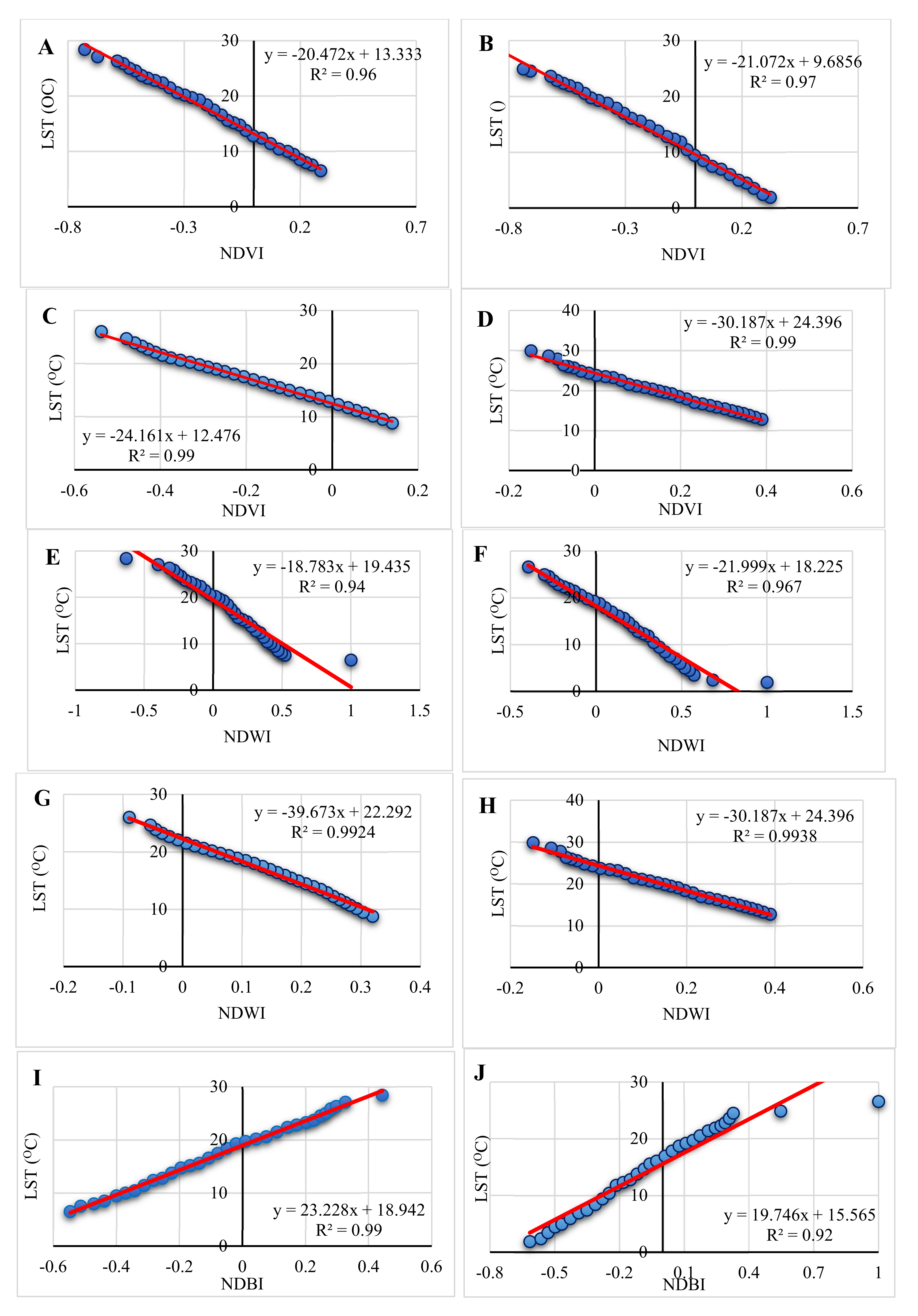
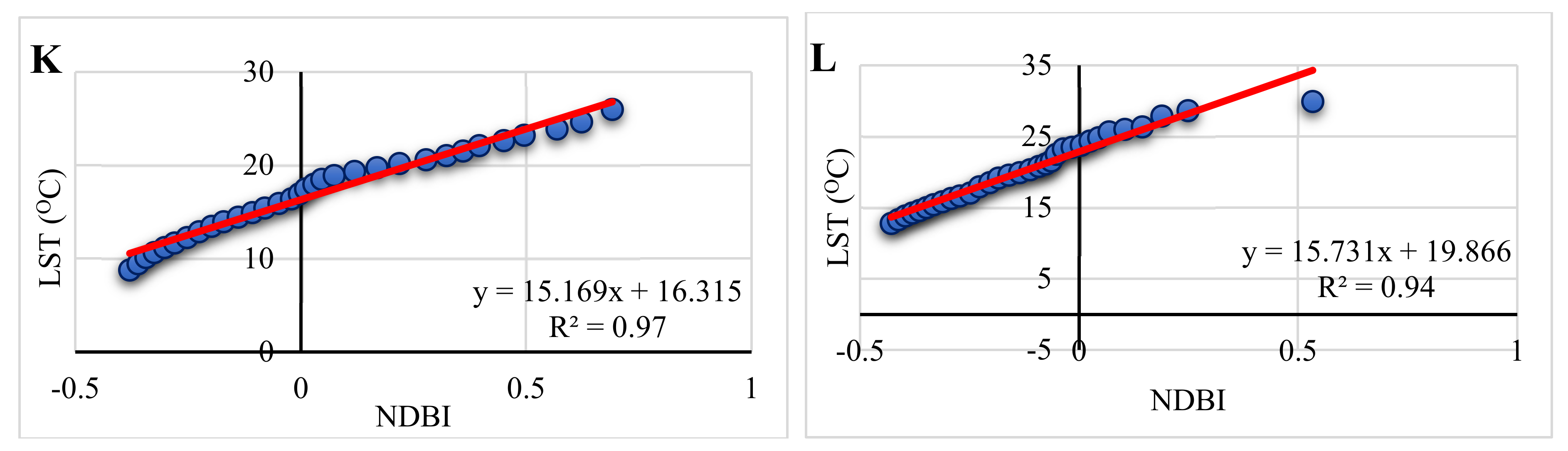
Relationship of LULC Indices (NDVI, NDWI, and NDBI) with LST

Regression analysis and Pearson’s product moment correlation were used to set up a co-relation between three land cover indices (NDBI, NDWI, and NDVI) and LST. One of the most extensively used indicators for tracking vegetation dynamics at both regional and global scales is the NDVI [45]. It was first introduced by [61]. Values range between 1 and −1. Higher values of the NDVI (≥0.6) represent a dense vegetation region, which leads to low surface temperature. Moderate NDVI values, ranging from 0.2 to 0.3, indicate hedge, grassland, and paved surfaces, which generate nominal surface temperature; however, barren land, rock, and built-up areas with NDVI values between 0 and 0.2 generate a high surface temperature. NDVI values ≤ 0 indicate water bodies [33,62]. The normalised difference water index (NDWI) is a dimensionless metric that ranges from −1 to +1 not only due to differences in leaf water content but also vegetation type and cover [63]. When the NDWI is high (blue), both the water content of the vegetation and the proportion of the land that is covered by vegetation are high. When the NDWI is low, the water content and fractional cover of plants are both low (in red) [64]. It is expected that NDWI is lower during times of water scarcity [65]. When exposed to drought, NDWI levels react more quickly than NDVI values [66]. The NDBI can take on a value between +1 and −1. According to the available data, those locations with a positive NDBI value are considered to be urban, while those with a negative NDBI value are considered to be rural [67]. On the other hand, an increase in the NDBI results in an increase in the LST of built-up areas [49].

The result shows that there is a negative association between LST and NDVI and LST and NDWI, as shown in Figure 12A–H, which suggests that the decline in the amount of water bodies and vegetation in the study area was responsible for the increase in LST measured there. The positive association between LST and NDBI that is shown in Figure 12I–L demonstrates that the increase in built-up area led to an increase in the LST over the time period being studied.

The study discovered a correlation between a greater value of LST and a lower value of the NDVI and NDWI. During the course of the research, the values of the NDVI and NDWI both went down, which means that there was less vegetation, less moisture in the soil, and fewer water bodies. On the other hand, the value of the NDBI continued to rise over time, which resulted in increasing LST levels. Higher correlation coefficients between LST and the NDVI (0.96, 0.97, 0.99, 0.99), NDWI (0.94, 0.96, 0.99, 0.99), and NDBI (0.99, 0.92, 0.97, 0.94) indicate a strong influence of LULC change on LST change.

The highest positive correlation between LST and the NDBI is 0.99, according to Pearson’s Product Moment analysis (

Table 8. LST, NDVI, and NDBI correlation coefficient.

1990		LST	NDVI	NDWI	NDBI
	LST		−0.99801	−0.96951	0.99827
	NDVI	−0.99801		0.97315	−0.9983
	NDWI	−0.96951	0.973146		−0.97417
	NDBI	0.998268	−0.9983	−0.97417
2000		LST	NDVI	NDWI	NDBI
	LST		−0.99592	−0.98338	0.96006
	NDVI	−0.99592		0.98328	−0.97626
	NDWI	−0.98338	0.98328		−0.95363
	NDBI	0.96006	−0.97626	−0.95363
2010		LST	NDVI	NDWI	NDBI
	LST		−0.99856	−0.99622	0.98505
	NDVI	−0.99856		0.99719	−0.9824
	NDWI	−0.99622	0.99719		−0.9918
	NDBI	0.98505	−0.9824	−0.9918
2020		LST	NDVI	NDWI	NDBI
	LST		−0.99688	−0.99688	0.97828
	NDVI	−0.99688		1	−0.96669
	NDWI	−0.99688	1		−0.96669
	NDBI	0.97828	−0.96669	−0.96669

). With a maximum value of 0.99, the correlation between LST and the NDVI shows a strong negative link. The greatest negative value of the estimated strong negative correlation between LST and the NDWI analysis is 0.98. According to the correlation that exists between LST and two indices (NDVI and NDWI), the average surface temperature is lower when there is a greater density of both vegetation and water bodies. High evapotranspiration rates are caused by dense woods, which also have higher NDVI values. Similar findings in other research corroborate the hypothesis [68,69,70,71].

4.4. Simulation of LULC for 2030 and 2040

For simulating the LULC map for the years 2030 and 2040 we used the 2010–2020 and 2020–2030 simulated LULC maps as the base maps, respectively (Figure 13). The LULC map indicates that the built-up area is mostly centred in and around Silchar city (central region of Cachar district) and it expanded in the southern and northeast regions because of the availability of favourable conditions and economic activities.

Table 9. Transition probability matrix for the year 2030.

Class	2030
	Dense Vegetation	Agricultural Land	Water Bodies	Built-Up	Others
Dense vegetation	0.897117	0.045052	0.025508	0.0323	0.000022
Agricultural Land Water bodies	0.025921 0.064633	0.699509 0.029343	0.079431 0.75831	0.19427 0.14484	0.000869 0.002873
Built-up	0.103973	0.191339	0.211551	0.49091	0.002228
Others	0.003019	0.097222	0.207528	0.27234	0.419887

and

Table 10. Transition probability matrix for the year 2040.

Class	2040
	Dense Vegetation	Agricultural Land	Water Bodies	Built-Up	Others
Dense vegetation	0.989262	0.002629	0.00415	0.003959	0
Agricultural Land	0	0.878694	0.01522	0.106087	0
Water bodies	0	0.008844	0.91209	0.079066	0
Built-up	0	0.002242	0.077722	0.920036	0
Others	0	0.000892	0.2301	0.07447	0.694537

show the transition probability matrix, which is forged using cross-tabulation of two LULC maps and two different years (in this case, it is the LULC of 2030 and 2040).

All potential maps show an accuracy of more than 85% with 100 iterations. Table 9 shows the transition for 2030, in which 49.09% of built-up land pixels belong to the same class, with 3.23% of dense vegetation, 19.47% of agricultural land, 14.48% of water bodies land, and 27.23% of land classified as “Others” being transformed into built-up land pixel values. Similarly, dense vegetation (89.97% pixel) and agricultural land classes (69.95% pixels) were found in the same classes. However, for water bodies, 75.83% of the pixel values remain in the same class, whereas very few percentages of pixels (0.28%) were renewed into a wasteland or bare land class. The transition matrix of 2040 (Table 10) shows that 92% of the built-up land area will remain in the same class, while 10.60% of agricultural land, 7.9% of water bodies, and 7.44% of land classified as “Others” is transformed into built-up land. Likewise, dense vegetation (98.82%) and agricultural land classes (87.86%) were found in the same classes. For water bodies, 91.2% of the land would be retained in the same class. The transition probabilities of the change in values between different LULC highlights the decreasing trends in dense vegetation and agricultural land use, and on the other hand, there is a rapid increase in urbanisation.

Table 11. Area statistics of simulated LULC for the years 2030 and 2040.

LULC Class	2030		2040		2030–2040
	Area in km2	Area in %	Area in km2	Area in %	Area in km2	Area in %
Dense Vegetation	2111.18	55.85	2107.11	55.74	−4.07	−0.11
Agricultural Land	750.40	19.85	730.02	19.31	−20.28	−0.54
Water bodies	362.36	9.59	360.79	9.54	−1.57	−0.04
Settlement	553.28	14.64	579.32	15.33	26.06	0.69
Others	2.80	0.07	2.79	0.07	−0.01	0.00

shows the area statistics of different LULC classes for the simulated years 2030 and 2040.

The simulated maps of the years 2030 and 2040 show that built-up land and land classified as “Others” will increase, while water bodies, agricultural, and vegetation areas will decrease in the study area. The built-up area will be increased by 107.23 km² and 26.04 km² in 2030 and 2040, with an increase in the “Others” area and a 1.57 km² and 20.28 km² decrease in water bodies and agricultural land, respectively, in 2040. The dense vegetation, agricultural land, and “Others” will decrease by 22.91 km², 92.67 km², and 1.23 km² in 2030, respectively, with a 4.07 km², 20.28 km², and 0.01 km² decrease in dense vegetation, agricultural land, and “Others” in 2040.

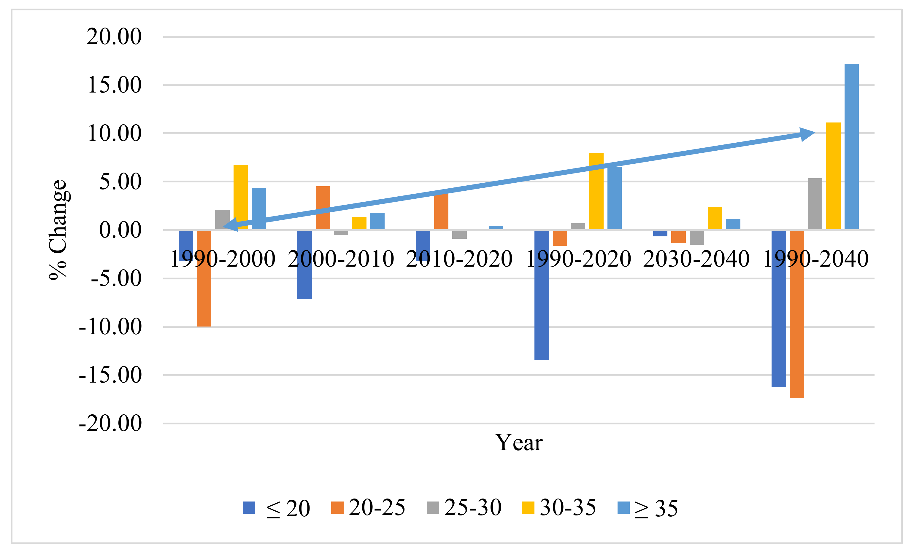
4.5. Prediction of LST Change for 2030 and 2040

During the study period, 1990–2020, significant change in LST can be seen within this study area. The previous pattern of LST (1990, 2000, 2010, and 2020) is used in the study to simulate LST in the ANN model. The predicted LST for 2030 and 2040 indicates that the majority of the Silchar city area (29.61% and 30.77%) will have an LST ≥ 35 °C for the years 2030 and 2040 (Figure 14). There is an increase in the area with a temperature more than 35 and in between 30–35 by 1.16% and 2.36% from 2030 to 2040 (

Table 12. Area statistics of simulated LST for the years 2030 and 2040.

LST in (°C)	2030		2040		2030–2040
	Area in (km2)	Area in %	Area in (km2)	Area in %	ΔArea (Km2)	Δ%
≤20	161.19	4.26	136.55	3.61	−24.64	−0.65
20–25	379.25	10.03	327.82	8.67	−51.43	−1.36
25–30	1074.17	28.42	1017.13	26.91	−57.05	−1.51
30–35	1046.07	27.67	1135.37	30.04	89.30	2.36
≥35	1119.34	29.61	1163.16	30.77	43.82	1.16

).

Various reasons such as global warming, the greenhouse effect, change in surface characteristics, even in the absence of rapid urbanisation, can increase the LST [72]. An increase in LST leads to the rise of UHI and also affects the thermal capacity of LULC [73]. Among all the major concerns that include its adverse effect on the environment, biodiversity, and human beings, the increase in UHI is one of them [74]. According to [75], the impact of global warming and UHI can be reduced by an urban green cover (planting trees and vegetation around the built-up areas).

5. Discussion

5.1. Change in LULC

As cities have grown, especially in developing countries, people have been constructing new buildings and structures all the time for decades. Due to this, the amount of land that can be soaked up by water and the amount of water and plants have decreased. This has slowly changed the temperature of the land surface and added to the UHI effect. According to a number of studies, the UHI intensity can change inside a city based on regional land use or land cover patterns, urban form, and the kinds of materials that are used [76]. According to the findings of several studies, the primary factor responsible for the rise in the UHI effect in Manchester, United Kingdom, was the increased utilisation of construction materials [77]. The Look East policy implemented by the PM of India in 1991 aimed to cultivate extensive economic and strategic relations with the nations of Southeast Asia in order to bolster its standing as a regional power, as a counterweight to the strategic influence of the People’s Republic of China. The goal of this policy is to strengthen India’s standing as a regional power and to compete with the strategic influence of the People’s Republic of China. The implementation of this policy leads to an extensive urban and infrastructure development with loss of vegetation cover. Various parts of the northeast experienced loss of vegetation in the past two to three decades [33,78]. As per the report, the northeast has lost more vegetation compared to other parts of India (India State of Forest Report, 2021) [79].

The current research examined how LULC has changed from 1990 to 2020. The results show that the built-up area grew by 7.13% between 1990 and 2020; during the period, the built-up area grew from 196 km² to 466.05 km², while the amount of vegetation decreased by 4.46% (Table 5). Considering the simulated years 2030 and 2040, in 50 years (1990–2040), built-up areas and water bodies will increase by 9.32% and 4.47%, respectively, with a significant decrease in dense vegetation, agricultural land, and other land uses by 5.65%, 10.58%, and 0.34%, respectively (Figure 15). Other South Asian cities’ urban areas area grew in the same way over the past two to three decades, with the loss of vegetation cover, such as Delhi, Patna, Lucknow, Kolkata, and Mangalore in India [21,23,80,81], or Cumillia, Dhaka, and Rajsahi of Bangladesh [69,71,82], and Kathmandu of Nepal [83]. Several things led to urbanisation, such as the growth of the population, the political and economic climate, and the movement of people from rural areas into cities, which leads to extensive construction work for the development of infrastructure at a higher rate, and population density also keeps on increasing in northeastern parts of India (Jyotishman, et al., 2011) [84]. The population of Cachar has increased 20.17% between 2001 to 2011 [85], and a 49% increment was observed from the LandScan population data from 2000 to 2020 (Figure 16 and

Table 13. Total sum and % change in density from 2000 to 2020.

Year	SUM	% Change
2000	1271811	49.67208
2005	1678924
2010	1815387
2019	1903546

). Several things, such as unplanned rural-to-urban migration, random infrastructure development, and unplanned urban expansion to accommodate the growing number of people living in cities, may have something to do with these changes. Natural resources are getting worse in many parts of the world because there are more people living there [86]. India has 1.21 billion people, making it the second most populous country in the world [87]. With a current growth rate of 2.13 percent, uncontrollable population growth could lead to high per capita consumption, damage to natural resources, and high demand for land, food, and basic services [88,89]. Different authors have said that the main reasons for urban growth in general are a mix of political and economic factors [75] and a high rate of population growth [90]. Our study area was not an exception, but rather a hot spot. Due to these things, cities grew quickly, and a mix of urban and rural LULC categories became the most important thing in our area of interest. More often than not, they were seen in newly built-up areas, especially in the greenbelts. Most of the areas that used to be covered in plants but were at a lower altitude near the built-up areas are now either built-up or have no plants at all.

5.2. Change in LST

The LST was calculated for each time period using thermal bands. The LST was retrieved using established algorithms relied on by scientists around the world [69], [91,92,93]. The results show that the LST has been getting higher from the base year of this study, 1990, to 2020, and that built-up areas are a big reason for this. Increasing urban footprints and an alarming drop in the number of plants will have a huge impact on the LST, which will lead to more UHI effects [69]. In our study, we found that the land surface temperature was highest where population density was higher, followed by bare soil, plants, and water. Similar results were found by [94,95], who looked at how LULC affected the temperature of the land surface in relation to urbanisation and population growth. These results were similar to what [96] found, which was that the LST was higher for bare soil and built-up areas than for water bodies and vegetation. The current study shows that the LST regimes grew as vegetated surfaces were turned into areas with no plants. The results of this study also show that the LST rose for all LULC classes from 1990 to 2020 (Figure 11 and Table 7). This likely happened because of global warming and changes to the surface [97]. The LST could go up if urban growth and climate change happened at the same time [98]. Researchers have found similar things in different cities in India [21,81,99]. From 1990 to 2020, the number of people living in the study area grew quickly (Table 13), which made the LST rise faster. Another thing, such as the fact that Landsat images have different temporal resolutions, could cause the LST to rise outside of the built-up area. However, the results show that the area was affected by both local warming and/or climate change.

5.3. Prediction of LULC Changes for the Years 2030 and 2040

The projected LULC of the study area shows that the LULC is likely to change over the next two decades and the built-up area in 2030 and 2040 will be 14.64% and 14.53% of the current land use land cover, which was 12.33% in 2020, that could be changed into the built-up class (Figure 15). Future predictions for other growing cities, such as Beijing in China, Dhaka in Bangladesh, Singapore, and Delhi in India, also showed a similar trend of an increasing number of built-up areas [23,69,98]. Since 1990, the population has grown in different decades, as seen in Bangladesh [100]. Rapid urbanisation leads to an urban sprawling of the city, which has both good and bad effects. One of the good effects is industrialisation, which gives more jobs to people who live in the area and in the surrounding areas. The growth of cities could lead to more business opportunities and better health care, but the population will also increase, and in that case, more job opportunities are needed to fulfil the basic lifestyle amenities and triggers to the housing market will undoubtedly alter the pattern of land use [101]. Increased household size may result in more compact urban centre growth when there is still room for it. Contrarily, if high-density development or high housing costs are not possible, especially in the city centre, then increased housing demand could result in sprawl [98]. In the study area, there could also be more building and setting up of new housing communities. The building of new, high-end neighbourhoods could make people’s lives more comfortable and raise their living standards. Some other bad effects of urbanisation are unemployment, higher fuel use, more solid medical waste, more air pollution, causing problems to human health and the environment [102,103]. India is expected to have the most people in the world, so more jobs are needed. In the same way, an increase in population and the growth of cities make it harder for people to get from one place to another, which can lead to more transportation use and traffic jams. This could cause more pollution in the air and cause health problems, especially for children and older people in our area. This could also put more stress on services provided by the government. Urbanisation also leads to social differences between people [104].

5.4. Prediction of LST Changes for the Year 2030 and 2040

Recurrent Neural Network (RNN), Convolutional Neural Network (CNN), Radial Basis Function Neural Network (RBFNN), and Modular Neural Network (MNN) GoogLeNet, VGGNet, and AlexNet are some of the commonly used methods in machine learning. Researchers employed these methods a lot when doing image processing and prediction investigations [9,62,105]. The ANN prediction model used in this study for simulating the LST for the years 2030 and 2040 showed that most of the study area could have LST regimes that are warmer than 35 °C, increasing linearly (Figure 17). Rapid urban growth is expected to cause a rise in temperature, which is in line with what a number of regional and global models said would happen [62,106,107]. This is because more people mean more demand for energy. Greenhouse gases, which are mostly made by people, are affected by the growth of cities. In fact, the huge amounts of carbon dioxide caused by humans are usually found in cities. This is because fossil fuels are burned to: (i) heat and cool buildings; (ii) make things in factories; and (iii) power cars. For example, [108,109] said that urbanisation and the growth of the middle class could cause the concentration of greenhouse gases and human-made heat emissions to rise. If the middle class’s income goes up, they might buy more appliances such as heaters, fridges, stoves, and air conditioners. Increases in the LST may be attributable to a number of factors, including the use of land for roads and cities, the needs of urban residents for goods and services, and vegetation work as the biggest carbon sink. This adaptation to LULC was primarily influenced by deforestation at the regional scale, which altered surface characteristics [110]. In the last 100 years, India’s average annual temperature has risen by 0.57 °C, and it will continue to rise by 3 °C to 4 °C in the central global emissions scenario [111,112]. Since air temperature and LST are related, a rise in air temperature would cause a rise in LST, and over the period 1860–2005, the average surface temperature (ST) in India has risen by 0.055 K/decade, corresponding to the worldwide warming trend [113]. The temperature of the land surface would be higher than the temperature of the air [92]. The rise in temperature could hurt plant and animal species, as well as people’s health.

6. Conclusions

In this study, we derived LULC hand in hand with LST within the span of 1990 to 2020 in the Cachar district of India. We also forecasted the LULC hand in hand with LST for 2030 and 2040 based on the changes. Through this study, we can say that, in 2040, the built-up area will increase by almost 9.33% from 1990, withering away dense vegetation (5.18%) and agricultural land (10.15%). The simulated LULC indicates that dense vegetation and agricultural land areas will decrease by 4.07 km², which is about 0.11% and 0.38 km², about 0.01%, by the years 2030 to 2040, respectively, in contrast to the initial years. The outcomes tell us that the average LST for three decades has increased by 5 °C. The LST spread of different LULC categories such as dense vegetation and water bodies the has lowest temperature, while the maximum temperature was registered in the built-up and bare land areas. The forecasted LST points to 27.67% and 30.04% of the total area likely experiencing temperatures between 30 °C to 35 °C between 2030 and 2040, respectively. On the other hand, merely 18.92% of the total area experienced it in the year 1990. If this trend goes on, the built-up areas, as well as the LST, will escalate in the coming decade, resulting in several environmental, economic, and medical issues for the region (mainly in the city). The results of this type of study will help the government, politicians, and urban administrative bodies of Silchar city, who may exhaust the findings of the study for their forthcoming policies and decisions therein. Municipalities or authorities can make strategies, rules, and laws that can reduce the LST in the city. Hence, the outputs herein may enable the Cachar district (especially Silchar city) to become environmentally and ecologically sustainable. Furthermore, human–environment interactions must be enquired into for detailed causes and impressions of LST variations. Urbanisation and variations in LST and LULC in other cities of India ought to be revisited and planned accordingly, for sustainable development.

7. Limitations

Due to the nature of the data and method used, there may be some limits to the observed results. After taking into account that the study is entirely based on Landsat data provided by USGS, which is freely available, as the images were taken on a particular date by the satellite, a more accurate and detailed analysis of change in LST can be constructed in the future by taking seasonal images into account, and a directional study can also be included for better presentation of the results. This time, the study of LULC change impacts on LST was carried out, and the analysis of the LST was not conducted on a seasonal basis, since, due to the freely available data, most of the Landsat images for the summer season have errors. A direction map may also be added for better representation of the results. Despite these limitations in the research process and estimation, the findings are genuine and scientific in nature. The verdicts of this study may be valuable to policymakers, environmental engineers, and city planners in their efforts to enhance the city’s urban management.

References

1. Sinha, J.; Jha, S.; Goyal, M.K. Influences of watershed characteristics on long-term annual and intra-annual water balances over India. J. Hydrol. 2019, 577, 123970. [Google Scholar] [CrossRef]
2. Ellwanger, J.H.; Kulmann-Leal, B.; Kaminski, V.L.; Valverde-Villegas, J.M.; Da Veiga, A.B.G.; Spilki, F.R.; Fearnside, P.M.; Caesar, L.; Giatti, L.L.; Wallau, G.L.; et al. Beyond diversity loss and climate change: Impacts of Amazon deforestation on infectious diseases and public health. An. Acad. Bras. Ciênc. 2020, 92, e20191375. [Google Scholar] [CrossRef] [PubMed]
3. Ganaie, T.A.; Jamal, S.; Ahmad, W.S. Changing land use/land cover patterns and growing human population in Wular catchment of Kashmir Valley, India. GeoJournal 2020, 86, 1589–1606. [Google Scholar] [CrossRef]
4. Saunders, D.A.; Hobbs, R.J.; Margules, C.R. Society for Conservation Biology Biological Consequences of Ecosystem Fragmentation: A Review Biological Consequences of Ecosystem Fragmentation: A Review. Source Conserv. Biol. Conserv. Biol. 1991, 5, 18–32. [Google Scholar] [CrossRef]
5. Thiha; Webb, E.L.; Honda, K. Biophysical and policy drivers of landscape change in a central Vietnamese district. Environ. Conserv. 2007, 34, 164–172. [Google Scholar] [CrossRef]
6. Reid, R.S.; Kruska, R.L.; Muthui, N.; Taye, A.; Wotton, S.; Wilson, C.J.; Mulatu, W. Land-use and land-cover dynamics in response to changes in climatic, biological and socio-political forces: The case of southwestern Ethiopia. Landsc. Ecol. 2000, 15, 339–355. [Google Scholar] [CrossRef]
7. Hassan, Z.; Shabbir, R.; Ahmad, S.S.; Malik, A.H.; Aziz, N.; Butt, A.; Erum, S. Dynamics of land use and land cover change (LULCC) using geospatial techniques: A case study of Islamabad Pakistan. SpringerPlus 2016, 5, 812. [Google Scholar] [CrossRef] [Green Version]
8. Lambin, E.F.; Geist, H.J.; Lepers, E. Dynamics of Land-Use and Land-Cover Change in Tropical Regions. Annu. Rev. Environ. Resour. 2003, 28, 205–241. [Google Scholar] [CrossRef] [Green Version]
9. Al Kafy, A.; Faisal, A.A.; Rahman, S.; Islam, M.; Al Rakib, A.; Islam, A.; Khan, H.H.; Sikdar, S.; Sarker, H.S.; Mawa, J.; et al. Prediction of seasonal urban thermal field variance index using machine learning algorithms in Cumilla, Bangladesh. Sustain. Cities Soc. 2020, 64, 102542. [Google Scholar] [CrossRef]
10. Fu, P.; Weng, Q. Responses of urban heat island in Atlanta to different land-use scenarios. Arch. Meteorol. Geophys. Bioclimatol. Ser. B 2017, 133, 123–135. [Google Scholar] [CrossRef]
11. McDonald, R.; Guneralp, B.; Zipperer, W.; Marcotullio, P. The Future of Global Urbanization and the Environment. Solutions 2015, 6, 60–69. [Google Scholar]
12. Pal, S.; Ziaul, S. Detection of land use and land cover change and land surface temperature in English Bazar urban centre. Egypt. J. Remote Sens. Space Sci. 2017, 20, 125–145. [Google Scholar] [CrossRef] [Green Version]
13. Coppin, P.; Jonckheere, I.; Nackaerts, K.; Muys, B.; Lambin, E. Digital change detection methods in ecosystem monitoring: A review. Int. J. Remote Sens. 2004, 25, 1565–1596. [Google Scholar] [CrossRef]
14. Policelli, F.; Hubbard, A.; Jung, H.C.; Zaitchik, B.; Ichoku, C. Lake Chad Total Surface Water Area as Derived from Land Surface Temperature and Radar Remote Sensing Data. Remote Sens. 2018, 10, 252. [Google Scholar] [CrossRef] [Green Version]
15. Aredehey, G.; Mezgebu, A.; Girma, A. Land-use land-cover classification analysis of Giba catchment using hyper temporal MODIS NDVI satellite images. Int. J. Remote Sens. 2017, 39, 810–821. [Google Scholar] [CrossRef]
16. Solaimani, K.; Arekhi, M.; Tamartash, R.; Miryaghobzadeh, M. Land use/cover change detection based on remote sensing data (A case study; Neka Basin). Agric. Biol. J. N. Am. 2010, 1, 1148–1157. [Google Scholar] [CrossRef]
17. Jia, K.; Liang, S.; Wei, X.; Yao, Y.; Su, Y.; Jiang, B.; Wang, X. Land Cover Classification of Landsat Data with Phenological Features Extracted from Time Series MODIS NDVI Data. Remote Sens. 2014, 6, 11518–11532. [Google Scholar] [CrossRef] [Green Version]
18. Habtamu, T.; Casper, I.M.; Joel, O.B.; Abubeker, H.; Ayana, A.; Yared, M. Evaluation of land use land cover changes using remote sensing Landsat images and pastoralists perceptions on range cover changes in Borana rangelands, Southern Ethiopia. Int. J. Biodivers. Conserv. 2018, 10, 1–11. [Google Scholar] [CrossRef] [Green Version]
19. Deng, J.S.; Wang, K.; Hong, Y.; Qi, J.G. Spatio-temporal dynamics and evolution of land use change and landscape pattern in response to rapid urbanization. Landsc. Urban Plan. 2009, 92, 187–198. [Google Scholar] [CrossRef]
20. Bastawesy, M.A.; Khalaf, F.I.; Arafat, S.M. The use of remote sensing and GIS for the estimation of water loss from Tushka lakes, southwestern desert, Egypt. J. Afr. Earth Sci. 2008, 52, 73–80. [Google Scholar] [CrossRef]
21. Choudhury, D.; Das, K.; Das, A. Assessment of land use land cover changes and its impact on variations of land surface temperature in Asansol-Durgapur Development Region. Egypt. J. Remote Sens. Space Sci. 2018, 22, 203–218. [Google Scholar] [CrossRef]
22. Al Kafy, A.; Rahman, S.; Faisal, A.-A.; Hasan, M.M.; Islam, M. Modelling future land use land cover changes and their impacts on land surface temperatures in Rajshahi, Bangladesh. Remote Sens. Appl. Soc. Environ. 2020, 18, 100314. [Google Scholar] [CrossRef]
23. Tripathy, P.; Kumar, A. Monitoring and modelling spatio-temporal urban growth of Delhi using Cellular Automata and geoinformatics. Cities 2019, 90, 52–63. [Google Scholar] [CrossRef]
24. Mozumder, C.; Tripathi, N.K. Geospatial scenario based modelling of urban and agricultural intrusions in Ramsar wetland Deepor Beel in Northeast India using a multi-layer perceptron neural network. Int. J. Appl. Earth Obs. Geoinf. 2014, 32, 92–104. [Google Scholar] [CrossRef]
25. Clarke, K.; Gaydos, L.J. Loose-coupling a cellular automaton model and GIS: Long-term urban growth prediction for San Francisco and Washington/Baltimore. Int. J. Geogr. Inf. Sci. 1998, 12, 699–714. [Google Scholar] [CrossRef] [Green Version]
26. Bora, A.; Meitei, L. Diversity of butterflies (Order: Lepidoptera) in assam university campus and its vicinity, cachar district, assam, India. J. Biodivers. Environ. Sci. 2014, 5, 328–339. [Google Scholar]
27. Annayat, W.; Sil, B.S. Assessing channel morphology and prediction of centerline channel migration of the Barak River using geospatial techniques. Bull. Eng. Geol. Environ. 2020, 79, 5161–5183. [Google Scholar] [CrossRef]
28. Ashwini, K.; Pathan, S.A.; Sil, B.S. Delineation of Groundwater Potential Zone and Flood Risk Zone in Cachar District area, India. J. Water Eng. Manag. 2020, 1, 16–34. [Google Scholar] [CrossRef]
29. Paul, S.; Ghosh, S.; Oglesby, R.; Pathak, A.; Chandrasekharan, A.; Ramsankaran, R. Weakening of Indian Summer Monsoon Rainfall due to Changes in Land Use Land Cover. Sci. Rep. 2016, 6, 32177. [Google Scholar] [CrossRef] [Green Version]
30. Mandal, J.; Ghosh, N.; Mukhopadhyay, A. Urban Growth Dynamics and Changing Land-Use Land-Cover of Megacity Kolkata and Its Environs. J. Indian Soc. Remote Sens. 2019, 47, 1707–1725. [Google Scholar] [CrossRef]
31. Mansour, S.; Al-Belushi, M.; Al-Awadhi, T. Monitoring land use and land cover changes in the mountainous cities of Oman using GIS and CA-Markov modelling techniques. Land Use Policy 2019, 91, 104414. [Google Scholar] [CrossRef]
32. Rizwan, U.; Malik, R.N.; Abdul, Q. Assessment of groundwater contamination in an industrial city, Sialkot, Pakistan. Afr. J. Environ. Sci. Technol. 2009, 3, 429–446. [Google Scholar]
33. Pathan, S.A.; Ashwini, K.; Sil, B.S. Spatio-temporal variation in land use/land cover pattern and channel migration in Majuli River Island, India. Environ. Monit. Assess. 2021, 193, 811. [Google Scholar] [CrossRef] [PubMed]
34. Wilkie, D.S.; Finn, J.T. Remote Sensing Imagery for Natural Resources Monitoring; Columbia University Press: New York, NY, USA, 1996. [Google Scholar]
35. Kumar, K.S.; Bhaskar, P.U.; Padmakumari, K. Estimation of Land Surface Temperature to Study Urban Heat Island Effect Using Landsat Etm+ Image. Int. J. Eng. Sci. Technol. 2012, 4, 771–778. [Google Scholar]
36. Townshend, J.R.G.; Justice, C.O. Analysis of the dynamics of African vegetation using the normalized difference vegetation index. Int. J. Remote Sens. 1986, 7, 1435–1445. [Google Scholar] [CrossRef]
37. Roy, D.P.; Wulder, M.A.; Loveland, T.R.; Woodcock, C.E.; Allen, R.G.; Anderson, M.C.; Helder, D.; Irons, J.R.; Johnson, D.M.; Kennedy, R.; et al. Landsat-8: Science and product vision for terrestrial global change research. Remote Sens. Environ. 2014, 145, 154–172. [Google Scholar] [CrossRef] [Green Version]
38. Avdan, U.; Jovanovska, G. Algorithm for Automated Mapping of Land Surface Temperature Using LANDSAT 8 Satellite Data. J. Sens. 2016, 2016, 1480307. [Google Scholar] [CrossRef] [Green Version]
39. Batty, M. Geocomputation Using Cellular Automata; Taylor & Francis: Abingdon, UK, 2000. [Google Scholar]
40. Hegde, N.P.; Muralikrishna, I.V.; Chalapatirao, K.V. Integration of Cellular Automata and Gis for Simulating Land Use Changes. In Proceedings of the 5th International Symposium Spatial Data Quality—ISPRS 2007, Enschede, The Netherlands, 13–15 June 2007. [Google Scholar]
41. Kumar, U.; Mukhopadhyay, C.; Ramachandra, T.V.; Infrastructure, S.T.; Planning, U. Cellular automata and Genetic Algorithms based urban growth visualization for appropriate land use policies Cellular automata and Genetic Algorithms based urban growth visualization for appropriate land use policies. In Proceedings of the Fourth Annual International Conference on Public Policy and Management, Centre for Public Policy, Indian Institute of Management (IIMB), Bangalore, India, 9–12 August 2009; pp. 9–12. [Google Scholar]
42. Nasiri, V.; Darvishsefat, A.A.; Rafiee, R.; Shirvany, A.; Hemat, M.A. Land use change modeling through an integrated Multi-Layer Perceptron Neural Network and Markov Chain analysis (case study: Arasbaran region, Iran). J. For. Res. 2018, 30, 943–957. [Google Scholar] [CrossRef]
43. Ahmed, B.; Kamruzzaman, M.; Zhu, X.; Rahman, M.S.; Choi, K. Simulating Land Cover Changes and Their Impacts on Land Surface Temperature in Dhaka, Bangladesh. Remote Sens. 2013, 5, 5969–5998. [Google Scholar] [CrossRef] [Green Version]
44. Ibrahim, F.; Rasul, G. Urban Land Use Land Cover Changes and Their Effect on Land Surface Temperature: Case Study Using Dohuk City in the Kurdistan Region of Iraq. Climate 2017, 5, 13. [Google Scholar] [CrossRef] [Green Version]
45. Imran, H.M.; Hossain, A.; Islam, A.K.M.S.; Rahman, A.; Bhuiyan, A.E.; Paul, S.; Alam, A. Impact of Land Cover Changes on Land Surface Temperature and Human Thermal Comfort in Dhaka City of Bangladesh. Earth Syst. Environ. 2021, 5, 667–693. [Google Scholar] [CrossRef]
46. Ashwini, K.; Pathan, S.A.; Singh, A. Understanding planform dynamics of the Ganga River in eastern part of India. Spat. Inf. Res. 2020, 29, 507–518. [Google Scholar] [CrossRef]
47. McFeeters, S.K. The use of the Normalized Difference Water Index (NDWI) in the delineation of open water features. Int. J. Remote Sens. 1996, 17, 1425–1432. [Google Scholar] [CrossRef]
48. Gao, B.-C. NDWI—A normalized difference water index for remote sensing of vegetation liquid water from space. Remote Sens. Environ. 1996, 58, 257–266. [Google Scholar] [CrossRef]
49. Zha, Y.; Gao, J.; Ni, S. Use of normalized difference built-up index in automatically mapping urban areas from TM imagery. Int. J. Remote Sens. 2003, 24, 583–594. [Google Scholar] [CrossRef]
50. Fattah, M.A.; Morshed, S.R.; Morshed, S.Y. Multi-layer perceptron-Markov chain-based artificial neural network for modelling future land-specific carbon emission pattern and its influences on surface temperature. SN Appl. Sci. 2021, 3, 359. [Google Scholar] [CrossRef]
51. Das, N.; Mondal, P.; Sutradhar, S.; Ghosh, R. Assessment of variation of land use/land cover and its impact on land surface temperature of Asansol subdivision. Egypt. J. Remote Sens. Space Sci. 2020, 24, 131–149. [Google Scholar] [CrossRef]
52. Maduako, I.D.; Yun, Z.; Patrick, B. Simulation and Prediction of Land Surface Temperature (LST) Dynamics within Ikom City in Nigeria Using Artificial Neural Network (ANN). J. Remote Sens. GIS 2016, 5, 1000158. [Google Scholar] [CrossRef]
53. Wang, R.; Murayama, Y. Geo-simulation of land use/cover scenarios and impacts on land surface temperature in Sapporo, Japan. Sustain. Cities Soc. 2020, 63, 102432. [Google Scholar] [CrossRef]
54. Sekertekin, A.; Arslan, N.; Bilgili, M. Modeling Diurnal Land Surface Temperature on a Local Scale of an Arid Environment Using Artificial Neural Network (ANN) and Time Series of Landsat-8 Derived Spectral Indexes. J. Atmos. Solar Terrestrial Phys. 2020, 206, 105328. [Google Scholar] [CrossRef]
55. Shatnawi, N.; Abu Qdais, H. Mapping urban land surface temperature using remote sensing techniques and artificial neural network modelling. Int. J. Remote Sens. 2019, 40, 3968–3983. [Google Scholar] [CrossRef]
56. Skidmore, A.K. Accuracy assessment of spatial information. In Spatial Statistics for Remote Sensing; Springer: Dordrecht, The Netherlands, 1999; pp. 197–209. [Google Scholar] [CrossRef]
57. Pontius, R.G. Quantification error versus location error in comparison of categorical maps. Photogramm. Eng. Remote Sens. 2000, 66, 1011–1016. [Google Scholar]
58. Landis, J.R.; Koch, G.G. An Application of Hierarchical Kappa-type Statistics in the Assessment of Majority Agreement among Multiple Observers. Biometrics 1977, 33, 363–374. [Google Scholar] [CrossRef] [PubMed]
59. Usman, M.; Liedl, R.; Shahid, M.A.; Abbas, A. Land use/land cover classification and its change detection using multi-temporal MODIS NDVI data. J. Geogr. Sci. 2015, 25, 1479–1506. [Google Scholar] [CrossRef]
60. Neteler, M. Estimating Daily Land Surface Temperatures in Mountainous Environments by Reconstructed MODIS LST Data. Remote Sens. 2010, 2, 333–351. [Google Scholar] [CrossRef] [Green Version]
61. Tucker, C. iw % SA Technical Memorandum 79620 Combinations for Monitoring Veqetation. Remote Sens. Environ. 1979, 8, 127–150. [Google Scholar] [CrossRef] [Green Version]
62. Ullah, S.; Ahmad, K.; Sajjad, R.U.; Abbasi, A.M.; Nazeer, A.; Tahir, A.A. Analysis and simulation of land cover changes and their impacts on land surface temperature in a lower Himalayan region. J. Environ. Manag. 2019, 245, 348–357. [Google Scholar] [CrossRef]
63. Delbart, N.; Kergoat, L.; Le Toan, T.; Lhermitte, J.; Picard, G. Determination of phenological dates in boreal regions using normalized difference water index. Remote Sens. Environ. 2005, 97, 26–38. [Google Scholar] [CrossRef] [Green Version]
64. Ceccato, P.; Gobron, N.; Flasse, S.; Pinty, B.; Tarantola, S. Designing a spectral index to estimate vegetation water content from remote sensing data: Part 1: Theoretical approach. Remote Sens. Environ. 2002, 82, 188–197. [Google Scholar] [CrossRef]
65. Gu, Y.; Hunt, E.; Wardlow, B.; Basara, J.B.; Brown, J.F.; Verdin, J.P. Evaluation of MODIS NDVI and NDWI for vegetation drought monitoring using Oklahoma Mesonet soil moisture data. Geophys. Res. Lett. 2008, 35, L22401. [Google Scholar] [CrossRef] [Green Version]
66. Gu, Y.; Brown, J.F.; Verdin, J.P.; Wardlow, B. A five-year analysis of MODIS NDVI and NDWI for grassland drought assessment over the central Great Plains of the United States. Geophys. Res. Lett. 2007, 34, L06407. [Google Scholar] [CrossRef] [Green Version]
67. Zheng, Y.; Tang, L.; Wang, H. An improved approach for monitoring urban built-up areas by combining NPP-VIIRS nighttime light, NDVI, NDWI, and NDBI. J. Clean. Prod. 2021, 328, 129488. [Google Scholar] [CrossRef]
68. Morsy, S.; Hadi, M. Impact of land use/land cover on land surface temperature and its relationship with spectral indices in Dakahlia Governorate, Egypt. Int. J. Eng. Geosci. 2021, 7, 272–282. [Google Scholar] [CrossRef]
69. Al Kafy, A.; Dey, N.N.; Al Rakib, A.; Rahaman, Z.A.; Nasher, N.M.R.; Bhatt, A. Modeling the relationship between land use/land cover and land surface temperature in Dhaka, Bangladesh using CA-ANN algorithm. Environ. Chall. 2021, 4, 100190. [Google Scholar] [CrossRef]
70. Hussain, S.; Mubeen, M.; Akram, W.; Ahmad, A.; Habib-Ur-Rahman, M.; Ghaffar, A.; Amin, A.; Awais, M.; Farid, H.U.; Farooq, A.; et al. Study of land cover/land use changes using RS and GIS: A case study of Multan district, Pakistan. Environ. Monit. Assess. 2019, 192, 2. [Google Scholar] [CrossRef]
71. Faisal, A.-A.; Al Kafy, A.; Al Rakib, A.; Akter, K.S.; Jahir, D.M.A.; Sikdar, S.; Ashrafi, T.J.; Mallik, S.; Rahman, M. Assessing and predicting land use/land cover, land surface temperature and urban thermal field variance index using Landsat imagery for Dhaka Metropolitan area. Environ. Chall. 2021, 4, 100192. [Google Scholar] [CrossRef]
72. Dereczynski, C.; Silva, W.L.; Marengo, J. Detection and Projections of Climate Change in Rio de Janeiro, Brazil. Am. J. Clim. Chang. 2013, 02, 25–33. [Google Scholar] [CrossRef] [Green Version]
73. Karl, T.R.; Diaz, H.F.; Kukla, G. Urbanization: Its Detection and Effect in the United States Climate Record. J. Clim. 1988, 1, 1099–1123. [Google Scholar] [CrossRef]
74. Grimmond, S. Urbanization and global environmental change: Local effects of urban warming. Geogr. J. 2007, 173, 83–88. [Google Scholar] [CrossRef]
75. Amiri, R.; Weng, Q.; Alimohammadi, A.; Alavipanah, S.K. Spatial–temporal dynamics of land surface temperature in relation to fractional vegetation cover and land use/cover in the Tabriz urban area, Iran. Remote Sens. Environ. 2009, 113, 2606–2617. [Google Scholar] [CrossRef]
76. Hart, M.A.; Sailor, D.J. Quantifying the influence of land-use and surface characteristics on spatial variability in the urban heat island. Theor. Appl. Climatol. 2009, 95, 397–406. [Google Scholar] [CrossRef]
77. Levermore, G.; Parkinson, J.; Lee, K.; Laycock, P.; Lindley, S. The increasing trend of the urban heat island intensity. Urban Clim. 2018, 24, 360–368. [Google Scholar] [CrossRef]
78. Annayat, W.; Ashwini, K.; Sil, B.S. Monitoring Land Use and Land Cover Analysis of the Barak Basin Using Geospatial Techniques. In Anthropogeomorphology; Springer: Cham, Switzerland, 2022; pp. 427–441. [Google Scholar] [CrossRef]
79. India State of Forest Report 2021, dia (Ministry of Environment Forest and Climate Change); Forest Survey of India (Ministry of Environment Forest and Climate Change): Dehradun, India, 2021.
80. Mishra, V.N.; Rai, P.K. A remote sensing aided multi-layer perceptron-Markov chain analysis for land use and land cover change prediction in Patna district (Bihar), India. Arab. J. Geosci. 2016, 9, 249. [Google Scholar] [CrossRef]
81. Shukla, A.; Jain, K. Analyzing the impact of changing landscape pattern and dynamics on land surface temperature in Lucknow city, India. Urban For. Urban Green. 2020, 58, 126877. [Google Scholar] [CrossRef]
82. Rahaman, Z.A.; Al Kafy, A.; Faisal, A.-A.; Al Rakib, A.; Jahir, D.M.A.; Fattah, A.; Kalaivani, S.; Rathi, R.; Mallik, S.; Rahman, M.T. Predicting Microscale Land Use/Land Cover Changes Using Cellular Automata Algorithm on the Northwest Coast of Peninsular Malaysia. Earth Syst. Environ. 2022, 6, 817–835. [Google Scholar] [CrossRef]
83. Thapa, R.B.; Murayama, Y. Examining Spatiotemporal Urbanization Patterns in Kathmandu Valley, Nepal: Remote Sensing and Spatial Metrics Approaches. Remote Sens. 2009, 1, 534–556. [Google Scholar] [CrossRef] [Green Version]
84. Deka, J.; Tripathi, O.P.; Khan, M.L. Urban growth trend analysis using Shannon Entropy approach—A case study in North-East India. Int. J. Geomatics Geosci. 2011, 2, 1062–1068. [Google Scholar]
85. Cencus. 2001. Available online: http://www.censusindia.gov.in/2011-common/census_data_2001.html (accessed on 11 September 2022).
86. Forsyth, T. Population and Natural Resources. In International Encyclopedia of Geography: People, the Earth, Environment and Technology; John Wiley & Sons, Ltd.: Oxford, UK, 2017; pp. 1–6. [Google Scholar]
87. Census of India. 2011. Available online: https://censusindia.gov.in/census.website/ (accessed on 11 September 2022).
88. Ramachandran, R.M.; Roy, P.S.; Chakravarthi, V.; Joshi, P.K.; Sanjay, J. Land use and climate change impacts on distribution of plant species of conservation value in Eastern Ghats, India: A simulation study. Environ. Monit. Assess. 2020, 192, 86. [Google Scholar] [CrossRef]
89. Alexandratos, N.; Fao, J.B. World Agriculture towards 2030/2050 the 2012 Revision; ESA Working Paper No. 12-03. Available online: https://www.fao.org/3/ap106e/ap106e.pdf (accessed on 11 September 2022).
90. AbouKorin, A.A. Impacts of Rapid Urbanisation in the Arab World: The Case of Dammam Metropolitan Area, Saudi Arabia. In Proceedings of the 5th International Conference and Workshop on Built Environment in Developing Countries (ICBEDC 2011), Penang, Malaysia, 6–7 December 2011. [Google Scholar]
91. Hu, M.; Wang, Y.; Xia, B.; Huang, G. Surface temperature variations and their relationships with land cover in the Pearl River Delta. Environ. Sci. Pollut. Res. 2020, 27, 37614–37625. [Google Scholar] [CrossRef]
92. Li, Z.; Guo, X.; Dixon, P.; He, Y. Applicability of Land Surface Temperature (LST) estimates from AVHRR satellite i mage composites in northern Canada. Prairie Perspect. 2007, 11, 119–130. [Google Scholar]
93. Xiao, R.; Weng, Q.; Ouyang, Z.; Li, W.; Schienke, E.W.; Zhang, Z. Land Surface Temperature Variation and Major Factors in Beijing, China. Photogramm. Eng. Remote Sens. 2008, 74, 451–461. [Google Scholar] [CrossRef] [Green Version]
94. Oke, T.R. The energetic basis of the urban heat island. Q. J. R. Meteorol. Soc. 1982, 108, 1–24. [Google Scholar] [CrossRef]
95. Oke, T.R. City size and the urban heat island. Atmos. Environ. 1973, 7, 769–779. [Google Scholar] [CrossRef]
96. Adegoke, J.O.; Pielke, R.A.; Eastman, J.; Mahmood, R.; Hubbard, K.G. Impact of Irrigation on Midsummer Surface Fluxes and Temperature under Dry Synoptic Conditions: A Regional Atmospheric Model Study of the U.S. High Plains. Mon. Weather Rev. 2003, 131, 556–564. [Google Scholar] [CrossRef]
97. Terando, A.J.; Costanza, J.; Belyea, C.; Dunn, R.R.; McKerrow, A.; Collazo, J.A. The Southern Megalopolis: Using the Past to Predict the Future of Urban Sprawl in the Southeast U.S. PLoS ONE 2014, 9, e102261. [Google Scholar] [CrossRef]
98. Han, H.; Yang, C.; Song, J. Scenario Simulation and the Prediction of Land Use and Land Cover Change in Beijing, China. Sustainability 2015, 7, 4260–4279. [Google Scholar] [CrossRef] [Green Version]
99. Mathew, A.; Sreekumar, S.; Khandelwal, S.; Kumar, R. Prediction of land surface temperatures for surface urban heat island assessment over Chandigarh city using support vector regression model. Sol. Energy 2019, 186, 404–415. [Google Scholar] [CrossRef]
100. Hasan, S.S.; Deng, X.; Li, Z.; Chen, D. Projections of Future Land Use in Bangladesh under the Background of Baseline, Ecological Protection and Economic Development. Sustainability 2017, 9, 505. [Google Scholar] [CrossRef] [Green Version]
101. Tsai, Y.-H. Housing demand forces and land use towards urban compactness: A push-accessibility-pull analysis framework. Urban Stud. 2014, 52, 2441–2457. [Google Scholar] [CrossRef]
102. Yadava, A.K.; Talreja, S.C.; Ashwini, K.; Rao, C.N.; Sakhare, D.T.; Rana, N. Investigation of various medical wastes and its impact on environmental pollution. Int. J. Health Sci. 2022, 12381–12392. [Google Scholar] [CrossRef]
103. Dey, S.; Purohit, B.; Balyan, P.; Dixit, K.; Bali, K.; Kumar, A.; Imam, F.; Chowdhury, S.; Ganguly, D.; Gargava, P.; et al. A Satellite–Based High-Resolution (1-km) Ambient PM2.5 Database for India over Two Decades (2000–2019): Applications for Air Quality Management. Remote Sens. 2020, 12, 3872. [Google Scholar] [CrossRef]
104. Bhatta, B. Analysis of Urban Growth and Sprawl from Remote Sensing Data; Springer: Berlin/Heidelberg, Germany, 2010. [Google Scholar]
105. Su, J.-H.; Piao, Y.-C.; Luo, Z.; Yan, B.-P. Modeling Habitat Suitability of Migratory Birds from Remote Sensing Images Using Convolutional Neural Networks. Animals 2018, 8, 66. [Google Scholar] [CrossRef] [Green Version]
106. Ullah, S.; Tahir, A.A.; Akbar, T.A.; Hassan, Q.K.; Dewan, A.; Khan, A.J. Remote Sensing-Based Quantification of the Relationships between Land Use Land Cover Changes and Surface Temperature over the Lower Himalayan Region. Sustainability 2019, 11, 5492. [Google Scholar] [CrossRef] [Green Version]
107. Lim, T.K.; Rajabifard, A.; Khoo, V.; Sabri, S.; Chen, Y. The smart city in Singapore: How environmental and geospatial innovation lead to urban livability and environmental sustainability. In Smart Cities for Technological and Social Innovation; Elsevier: Amsterdam, The Netherlands, 2021; pp. 29–49. [Google Scholar]
108. Kahn, M.E. Urban Growth and Climate Change. Annu. Rev. Resour. Econ. 2009, 1, 333–350. [Google Scholar] [CrossRef] [Green Version]
109. Abutaleb, K.; Ngie, A.; Darwish, A.; Ahmed, M.; Arafat, S.; Ahmed, F. Assessment of Urban Heat Island Using Remotely Sensed Imagery over Greater Cairo, Egypt. Adv. Remote Sens. 2015, 4, 35–47. [Google Scholar] [CrossRef]
110. Svirejeva-Hopkins, A.; Schellnhuber, H.J. Urbanised territories as a specific component of the global carbon cycle. PIK Rep. 2005, 94, 5–126. [Google Scholar] [CrossRef] [Green Version]
111. National Intelligence Council. India: The Impact of Climate Change to 2030—A Commissioned Research Report. 2009. Available online: https://www.hsdl.org/c/abstract/?docid=24157 (accessed on 11 September 2022).
112. Yaduvanshi, A.; Zaroug, M.; Bendapudi, R.; New, M. Impacts of 1.5 °C and 2 °C global warming on regional rainfall and temperature change across India. Environ. Res. Commun. 2019, 1, 125002. [Google Scholar] [CrossRef]
113. Basha, G.; Kishore, P.; Ratnam, M.V.; Jayaraman, A.; Kouchak, A.A.; Ouarda, T.B.M.J.; Velicogna, I. Historical and Projected Surface Temperature over India during the 20th and 21st century. Sci. Rep. 2017, 7, 2987. [Google Scholar] [CrossRef]
Figure 1. Study area: (a) India, (b) Assam, and (c) Cachar.
Sustainability 14 14087 g001
Figure 2. Flow chart of methodology for LULC, LST, and population density analysis.
Sustainability 14 14087 g002
Figure 3. Flow chart for prediction of LULC change for 2030 and 2040 using CA Model.
Sustainability 14 14087 g003
Figure 4. (a) DEM, (b) Slope, (c) Aspect, (d) CBD, (e) Proximity to Water Bodies, (f) Proximity to Road.
Sustainability 14 14087 g004
Figure 5. Three-layer ANN structure.
Sustainability 14 14087 g005
Figure 6. ANN training and testing data set results for the prediction of LST for the year 2020.
Sustainability 14 14087 g006
Figure 7. LULC of Cachar for the years (a) 1990, (b) 2000, (c) 2010, and (d) 2020.
Sustainability 14 14087 g007
Figure 8. Change in built-up areas of Cachar for the years (a) 1990, (b) 2000, (c) 2010, and (d) 2020.
Sustainability 14 14087 g008
Figure 9. Decadal Change in LULC for the years (a) 1990–2000, (b) 2000–2010, (c) 2010–2020, and (d) 2020–1990.
Sustainability 14 14087 g009
Figure 10. Decadal change in %.
Sustainability 14 14087 g010
Figure 11. LST of Cachar for the years (a) 1990, (b) 2000, (c) 2010, and (d) 2020.
Sustainability 14 14087 g011
Figure 12. 1990, 2000, 2010, and 2020 LST correlation with NDVI, NDWI, and NDBI.
Sustainability 14 14087 g012aSustainability 14 14087 g012b
Figure 13. Predicted LULC of Cachar for the years (a) 2030 and (b) 2040.
Sustainability 14 14087 g013
Figure 14. Predicted LST of Cachar for the years (a) 2030 and (b) 2040.
Sustainability 14 14087 g014
Figure 15. Net gain or loss of different LULC classes from 1990 to 2040.
Sustainability 14 14087 g015
Figure 16. Population density in (a) 2000, (b) 2005, (c) 2010, and (d) 2020.
Sustainability 14 14087 g016
Figure 17. Trend of LST over years.
Sustainability 14 14087 g017