Optimized Stacking Ensemble Learning Model for Breast Cancer Detection and Classification Using Machine Learning

Abstract

Breast cancer is the most frequently encountered medical hazard for women in their forties, affecting one in every eight women. It is the greatest cause of death worldwide, and early detection and diagnosis of the disease are extremely challenging. Breast cancer currently exceeds all other female cancers, including ovarian cancer. Researchers can use access to healthcare records to find previously unknown healthcare trends. According to the National Cancer Institute (NCI), breast cancer mortality rates can be lowered if the disease is detected early. The novelty of our work is to develop an optimized stacking ensemble learning (OSEL) model capable of early breast cancer prediction. A dataset from the University of California, Irvine repository was used, and comparisons to modern classifier models were undertaken. The implementation analyses reveal the unique approach’s efficacy and superiority when compared to existing contemporary categorization models (AdaBoostM1, gradient boosting, stochastic gradient boosting, CatBoost, and XGBoost). In every classification task, predictive models may be used to predict the class level, and the current research explores a range of predictive models. It is better to integrate multiple classification algorithms to generate a set of prediction models capable of predicting each class level with 91–99% accuracy. On the breast cancer Wisconsin dataset, the suggested OSEL model attained a maximum accuracy of 99.45%, much higher than any single classifier. Thus, the study helps healthcare professionals find breast cancer and prevent it from happening.

1. Introduction

Breast cancer treatment can be quite effective, especially if caught early in the disease’s course. Most breast cancer therapies include surgical excision, radiation therapy, and medication. These therapies are intended to target tiny cancers that have spread from a breast tumor into the bloodstream. The fact that such treatment can halt cancer growth and spread while also saving lives attests to this. Breast cancer will claim the lives of 2.3 million new patients and 685,000 people will die as a result of the disease by 2020. Breast cancer will be the most common type of cancer in the world by 2020, according to the World Health Organization (WHO) [1]. In the last five years, 7.8 million cases of breast cancer have been diagnosed. Because it develops in the breast cells, breast cancer is one of the most prevalent forms of cancer in women. After lung cancer, breast cancer is the most common cancer in women. Breast cancer types can be distinguished using a microscope. There are two most frequent kinds of breast cancer, invasive ductal carcinoma (IDC) and ductal carcinoma in situ (DCIS), with DCIS taking longer to develop and having a smaller impact on patients’ daily lives. As many as 80% of breast cancer cases are diagnosed with IDC. The IDC form is more dangerous since it involves the entire breast tissue and is consequently more lethal than the DCIS type, which only accounts for between 20 and 53% of cases. This category includes most breast cancer patients (roughly 80%). Breast cancer is the type of cancer that is responsible for the greatest number of disability-adjusted years of life lost in female patients when compared to all other types of cancer combined [2].

Breast cancer can strike a woman at any age after puberty in any part of the globe. However, as one ages, the risk increases. Between 1930 and 1970, the number of women losing their lives to breast cancer remained largely stable. In countries that adopted early detection programs and a variety of treatment options to eradicate invasive diseases, life expectancy began to rise in the 1980s. Breast cancer is not contagious, unlike other malignancies. As opposed to human papilloma virus (HPV) infection and cervical cancer, breast cancer has no known viral or bacterial infections. Nearly half of all breast cancer cases are caused by women who have no known risk factors for the disease other than their gender (female) and age (over 40 years old). Breast cancer is more common in women who have a family history of the disease, drink excessive amounts of alcohol, or use hormone therapy after menopause, all of which raise the risk. Breast cancer symptoms include a lump or thickening of the breast that is painless. Women should seek medical attention as soon as they notice a lump in their breasts, regardless of how painful it is [3]. Breast lumps can arise for several reasons, the majority of which are benign. Breast lumps have a 90% chance of being benign. Breast abnormalities that are not cancerous include infections and benign tumors such as fibroadenomas and cysts. A thorough medical examination is required [4].

Imaging of the breast and, in certain instances, the removal of a sample of tissue are both methods that can be utilized to ascertain whether a tumor is cancerous or benign. Tests, such as imaging of the breast and tissue sampling (biopsy), should be performed on women who have persistent abnormalities (typically lasting more than one month) [5]. In the past several decades, there have been several advancements made in machine learning algorithms used for the diagnosis and categorization of breast cancer. Preprocessing, feature extraction, and classification are the three processes that comprise these methods. It is possible to improve interpretation and analysis by preprocessing the mammography films to make the pictures’ peripheral areas and intensity distributions more visible. There have been many different tactics described, and quite a few of them are effective [6]. The use of machine learning is growing more and more widespread, to the point that it will likely soon be commercialized as a service. Unfortunately, machine learning remains a difficult field, one that almost always calls for the application of specialized knowledge and skills. To make a reliable method for machine learning, we need a wide range of skills and experience [7], such as preprocessing, feature engineering, and classification approaches.

Breast cancer is treatable, and if caught and treated in its early stages, a positive prognosis is possible. Because of this, the accessibility of adequate screening technologies is essential to the early detection of the signs and symptoms associated with breast cancer. Mammography, ultrasound imaging, and thermography are three of the most common imaging procedures that may be utilized in the screening and diagnosis processes for this ailment. Other imaging methods may also be utilized. Although mammography is one of the most effective ways to detect breast cancer at an early stage, it is also one of the costliest. Ultrasound or diagnostic sonography techniques are gaining popularity as an alternative to mammography for women who have firm breasts because mammography is useless in this situation. Small cancerous tumors can be found without the use of radiation from X-rays, and thermography may be better at finding small cancerous tumors than ultrasonography.

A wide range of industries, including medicine, agriculture, and smart cities, can benefit from data mining, all of which can be put to good use by the general public. Research has been done utilizing several classification methodologies, such as the k-nearest neighbor, random forest, logistic regression, support vector machine, and decision tree. A stacking ensemble approach for determining the base classifier is proposed in this study, in contrast with the traditional single prediction models that are used to predict class level in any classification task. The traditional models are to be replaced by this approach. When several learning algorithms work together to solve a single problem, this is called “ensemble learning”.

1.1. Stacking Ensemble Learning Architecture

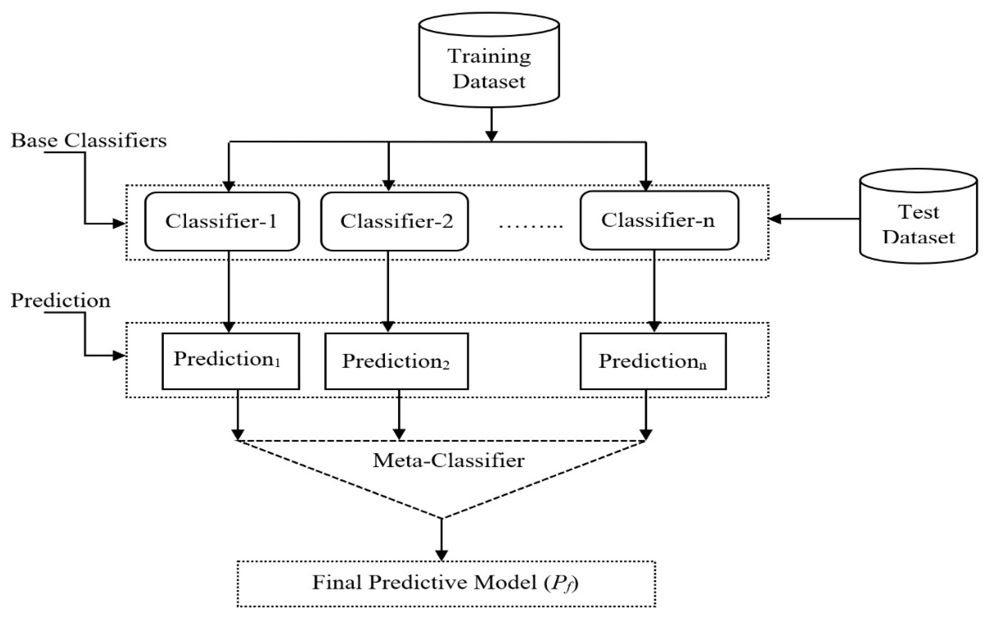
The stacking ensemble model’s architecture is depicted in Figure 1. The meta-classifier and the base-classifiers make up the stacking ensemble learning. The training set is used in the meta-classifier to train models and make predictions. There are two ways in which data are used for classification: one is the metaclassifier, which is based on the meta-data, and the other is the base-classifiers. The Netflix team known as “The Ensemble,” which is tied for the winning submission in terms of accuracy, employs this strategy. To guarantee that the ensemble has a wide diversity of components, heterogeneous ensemble methods employ several distinct base learning algorithms. It is made up of people who make use of a variety of basic learning algorithms, such as support vector machines, artificial neural networks, and decision trees, to produce the highest quality of work that is humanly possible. Stacking is a well-known heterogeneous ensemble method that is utilized in a variety of different applications. It is analogous to the concept of boosting.

1.2. Motivation for This Study

Many previously published authors did not work on process structure to carry out discoveries, instead relying on data-centric methods. This emphasizes the importance of the present investigation. The bulk of the time, writers focus on classification issues at a single level, and the machine learning models they apply are tailored to the datasets they employ. In several early research studies, the preprocessing phases were omitted altogether, and either a single feature selection strategy or several feature selection approaches were employed. Most of the efforts were motivated by preexisting objectives. The methodology that has been proposed will automatically decide the preprocessing and classification methods and parameters to be used. An expert in machine learning determines which approach is optimal for a certain problem domain at hand. Those who are not experts in machine learning must put in a substantial amount of effort to optimize the proposed models and achieve the desired performance. By using a dozen different methods, this research will help us get closer to its goal, which is to automate the process of making machine learning models.

1.3. Problem Statement

One in every eight women will be diagnosed with breast cancer over their lifetime. This makes it the health risk that is most common for women in their forties. Early identification and diagnosis of the illness may be incredibly difficult, even though it is the leading cause of mortality throughout the globe. There has been a discernible rise in the utilization of classification-based methodologies within current medical diagnostics. Studies on cancer are the primary focus of efforts to apply modern techniques from the fields of bioinformatics, statistics, and machine learning to achieve a more precise and speedy diagnosis. With predictive and personalized medicine becoming more and more important, there is a fast-growing need to use machine learning-driven models in cancer research to make predictions and determine a patient’s prognosis.

The rest of the paper is organized as follows: Section 2 defines the significance of past work on the topic of ensemble learning. Section 3 describes the preprocessing work done on the identified data sets. The proposed approach is explained in Section 4. Section 5 presents the implementation of the proposed solution. Section 6 includes a comparison of the proposed model to the existing models. Section 7 concludes the analysis and includes a discussion of potential future scope orientations.

2. Related Work

Data have displaced conventional power centers. Massive growth in the utilization of data analysis across all fields has benefited from the application of data mining. There are many applications for data mining, including identifying patterns and trends in a variety of fields, such as health care and social media. The weighted idea of the naïve Bayes classifier (NBC) for the diagnosis of breast cancer was changed by Kharya, S. et al. [8] who developed a new prediction model, the weighted naïve Bayes classifier (WNBC). On a benchmark dataset, the framework was developed and experiments were carried out to compare its performance to that of current non-weighted non-NBC and recently accessible models such as radial basis function (RBF), the weighted associative classifier (WAC), and feature weighted association classification (FWAC). Chaurasia, V. et al. [9] used three well-known data mining methods, including naïve Bayes, RBF networks, and J48, on the Wisconsin breast cancer dataset (WBCD). The naïve Bayes method performed the best, with a classification accuracy of 97.36%. Second and third place went to the RBF network and J48 algorithms, respectively, with a classification accuracy of 96.77% and 93.41%. Data from the University of California, Irvine (UCI) machine learning repository were used by Verma, D. et al. [10] to classify two types of cancer: breast cancer and diabetes. Methods such as naïve Bayes and sequential minimal optimization (SMO) were also used. Data mining techniques to assess the chance of breast cancer recurrence are important, but Ojha, U. et al. [11], emphasized the importance of parameter selection. The use of clustering and classification methods is explained and it was found that classification and techniques outperformed clustering.

By comparing two machine learning algorithms, Kumar, V. et al. [12] developed a Breast classifier model that can distinguish between benign and malignant breast tumors. The Wisconsin breast cancer diagnosis dataset is used to accomplish this purpose. Classifier overfitting and underfitting are also addressed by researchers, as well as data interpretation and handling of missing values. Sahu, B. et al. [13] used a neural network to classify breast cancer data. Using artificial neural networks, the article examines and assesses various methods for detecting breast cancer. Abdar, M. et al. [14] selected the top three classifiers based on F3 scores. False negatives in breast cancer categorization are emphasized by the F3 score (recall). Ensemble classification is then performed using these three classifiers and a voting mechanism. Hard and soft voting methods were also put to the test. These probabilities were averaged or multiplied for both hard and soft voting. The highest and lowest were also used. When hard voting (majority-based voting) is used, it is 99.42% better than the WBCD algorithm.

Abdar, M. et al. [15] proposed recursive ensemble classifiers to evaluate the classification accuracy, precision, and recall of single and nested ensemble classifiers, as well as computation times. It was also important for the authors to compare the proposed model’s accuracy to that of other well-known models. Single classifiers cannot compete with the two-layer ensemble models proposed here. It was found that SV-BayesNet-3 and Naïve Bayes-3 were both 98% accurate. SV-Naive Bayes-3-MetaClassifier, on the other hand, was built much more swiftly A modified bat technique (MBT) was proposed by Jeyasingh, S. et al. [16] as a feature selection process for reducing redundant characteristics in a dataset. They rewrote the bat algorithm to select data points at random from the dataset using basic random sampling. The dataset was ranked using the world’s greatest criteria to determine its prominent qualities. A random forest algorithm was developed using these properties. Breast cancer detection is easier with the MBT feature selection technique. The proposed jointly sparse discriminant analysis (JSDA) technique by Kong, H. et al. [17] not only improves diagnosis accuracy when compared to the classic feature extraction and discriminant analysis algorithms, but it also learns jointly sparse discriminant vectors to investigate the critical elements of breast cancer pathologic diagnosis, as demonstrated. Several well-known subspace learning algorithms fail to beat JSDA when applied to breast cancer datasets that are sparse, even when sample counts are low. Analysis of JSDA data shows that the main risk factors for breast cancer that were looked at are true to life.

When determining the textural characteristics of mammograms, the grey level cooccurrence matrix (GLCM) feature calculated along a zero-degree axis yielded the most accurate findings by Toner, E. et al. [18]. In an artificial neural network, the best features are then selected and used for training and classification using an artificial neural network (ANN). In addition to medical diagnosis and pattern recognition, ANNs are used in a wide range of applications. For this investigation, researchers used the mini-MIAS database, and the results indicated 99.3% sensitivity, 100% specificity, and 99.4% accuracy. Early cancer detection is essential if we wish to reduce the death rate from breast cancer. Mammograms from the miniMIAS database were used by Tariq, N. et al. [19] in their research experiment. This database contains 322 mammograms, of which 270 are normal and 52 are malignant. Following the calculation of ten texture features from the gray-level cooccurrence matrix along 0°, the ranked features approach further reduced the number of texture features to six. The obtained results show that this technique achieves 99.4% overall accuracy, with 100% accuracy for validation and test data. The novel sliding window technique for feature extraction presented in this research makes use of the local binary pattern features. This approach produces 25 sliding panes for each image. A support vector machine classifier is made from the traits that are taken from each window and saved.

According to the findings of Alqudah, A. et al. [20], the SVM classifier separates each picture into benign and malignant categories based on each image’s most prominent window classes. The approach may be used to locate the cancerous tissues using the whole histopathological image. The recommended strategy has overall accuracy, sensitivity, and specificity of 91.12%, 85.22%, and 94.01%, respectively. Rasti, R. et al. [21] used the ME-CNN model, which consists of three CNN experts and one convolutional gating network, to achieve 96.39% accuracy, 97.73% sensitivity, and 94.87% specificity. In terms of classification performance, the experimental results show that it outperforms two convolutional ensemble methods and three existing single-classifier approaches. The ME-CNN model may be useful to radiologists when analyzing breast DCE-MRI images. Wahab, N. et al. [22] recommended a strategy that greatly decreased training time when compared to the methodology that had the best F-measure of 0.78. The suggested method opens possibilities for employing CNNs’ automatic feature extraction capabilities in imbalanced medical photos to precisely diagnose these awful diseases for the benefit of all living creatures. It is used for other sorts of medical images besides breast cancer images.

Bhardwaj, A. et al. [23] suggested a solution for dealing with classification problems by using a genetically optimized neural network (GONN) strategy. It is used to determine if a tumor is benign or malignant in breast cancer situations. The performance of GONN against the classical model and the classical backpropagation model from UCI’s machine learning library was used to show how important the obtained results are. AUC under ROC curves, ROC curves, and the confusion matrix were also compared. Curvelet moments have been shown in trials to be superior to other ways of analyzing mammograms and to be both beneficial and effective. Curvelet moments have a 91.27 % accuracy rate for detecting abnormalities or cancers when used with 10 or 8 in the case of malignancy detection, according to the mini-MIAS database. More real-world tests on the DDSM database show that Dhahbi, S. et al.’s [24] proposed method is more accurate than all previous curvelet-based methods and reduces the total number of features.

The combined SVM and extra-trees model that Alfian, G. et al. [25] suggested attained maximum accuracy of up to 80.23%, which was far superior to the other ML model. When compared to ML that did not use the method of feature selection, the experimental findings revealed that the average ML prediction accuracy could be improved by as much as 7.29% when extra-trees-based feature selection was used to choose features. To improve the accuracy of breast cancer classification, Safdar, S. et al. [26] proposed a model that makes use of machine learning techniques such as SVM, logistic regression (LR), and K-nearest neighbor (KNN). They achieved the greatest accuracy possible, which was 97.7%, with a false positive rate of 0.01, a false negative rate of 0.03, and an area under the ROC curve (AUC) score of 0.99. Mohamed, E. A. et al. [27] proposed a two-class deep learning model that is trained from scratch to differentiate between normal and diseased breast tissues based on thermal images. Additionally, it is used to extract additional features from the dataset that are beneficial in the process of training the network and improving the effectiveness of the classification procedure. Accuracy levels of up to 99.33% have been reached using the suggested approach.

Table 1. Research papers were taken into consideration for review.

Authors	Publisher/Year	Algorithms
Kharya, S. et al. [8]	IJCA/2019	NB and Weighted Naive Bayesian (WNB) Approach
Chaurasia, V. et al. [9]	SAGE/2018	Naïve Bayes, RBF Network, J48
Verma, D. et al. [10]	IEEE/2017	Naïve Bayes, SMO, REP Tree, J48, MLP
Ojha, U. et al. [11]	IEEE/2017	Decision Tree, SVM and Fuzzy c-means
Kumar, V. et al. [12]	Stringer/2020	AdaBoostM1, Decision Table, Multiclass Classifier, Multilayer–Perceptron, Random Forest/Tree
Sahu, B. et al. [13]	EAI/2019	PCA-ANN hybrid feature selection (ANN)
Abdar, M. et al. [14]	MDPI/2019	Hard voting, Majority-based Voting
Abdar, M. et al. [15]	Elsevier/2020	SV-BayesNet-3-MetaClassifier, SV-Naïve Bayes-3-MetaClassifier
Jeyasingh, S. et al. [16]	APOCP/2017	Modified Bat Algorithm, Random Forest
Kong, H. et al. [17]	Elsevier/2016	Jointly Sparse Discriminant Analysis (JSDA)
Gerasimova-Chechkina, E. et al. [18]	AIP/2016	1D wavelet transform modulus maxima (WTMM) method
Tariq, N. et al. [19]	Hilaris-JMBD/2017	Artificial Neural Network
Alqudah, A. et al. [20]	Taylor & Francis/2019	Local Binary Pattern, SVM, and Sliding Window Technique
Rasti, R. et al. [21]	Elsevier/2017	Neural network ensemble composed of convolutions (ME-CNN)
Wahab, N. et al. [22]	Elsevier/2017	Deep Convolutional Neural Network (CNN)
Bhardwaj, A. et al. [23]	Elsevier/2015	Genetically Optimized Neural Network (GONN)
Dhahbi, S. et al. [24]	Elsevier/2015	k-nearest neighbor classifier and t-test ranking
Alfian, G. et al. [25]	MDPI/2022	SVM and extra-trees model
Safdar, S. et al. [26]	MDPI/2022	SVM, Logistic Regression (LR), and K-Nearest Neighbor (KNN)
Mohamed, E. A. [27]	PLOS ONE/2022	U-Net network, CNN-based deep learning model

shows the publisher, the year in which the research was published, and the algorithms that were used to make the research work.

3. Material and Methods

This section describes the existing methods available in the literature:

3.1. Dataset Description

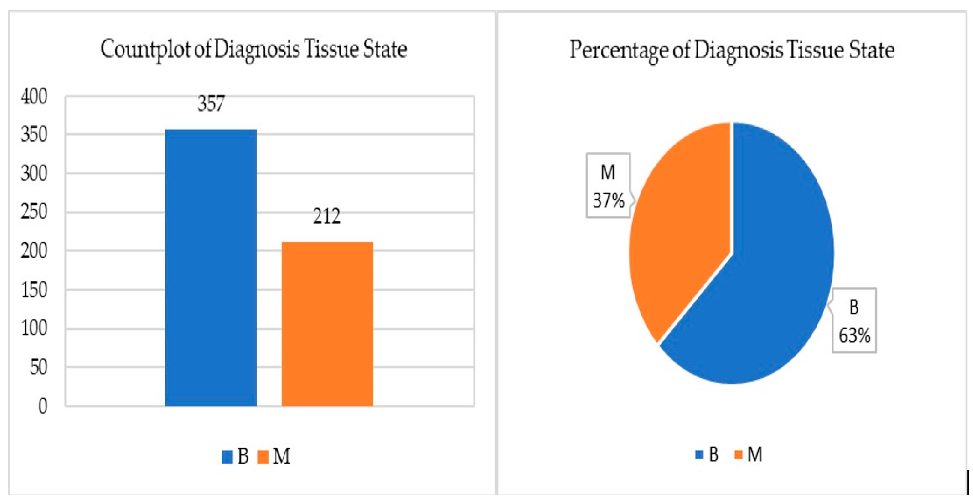
The breast cancer Wisconsin data repository at UC Irvine (UCI) Machine Learning has 569 occurrences and is organized into two classes [28]. In this dataset, samples are characterized by a total of 32 features, the first of which is the ID of the sample, the second of which is the class of the sample, and the remaining 30 features are features that contain various information about the cells. The selected dataset can be classified as either malignant (M) or benign (B). These are some of the medical terms that are used to refer to benign and malignant tumor cells. There is not a single value that is missing from the dataset. Of the total records in the dataset that was chosen, 357 (62.7%) are benign, whereas 212 (37.3%) are malignant.

3.2. Exploratory Data Analysis

Data visualization is an additional method that may be used to comprehend data. By making use of data visualization, we can see how the data appear and how the characteristics of the data correlate. The output can be checked against the features in the shortest possible time using this procedure.

3.2.1. Distribution Plots of Different Attributes

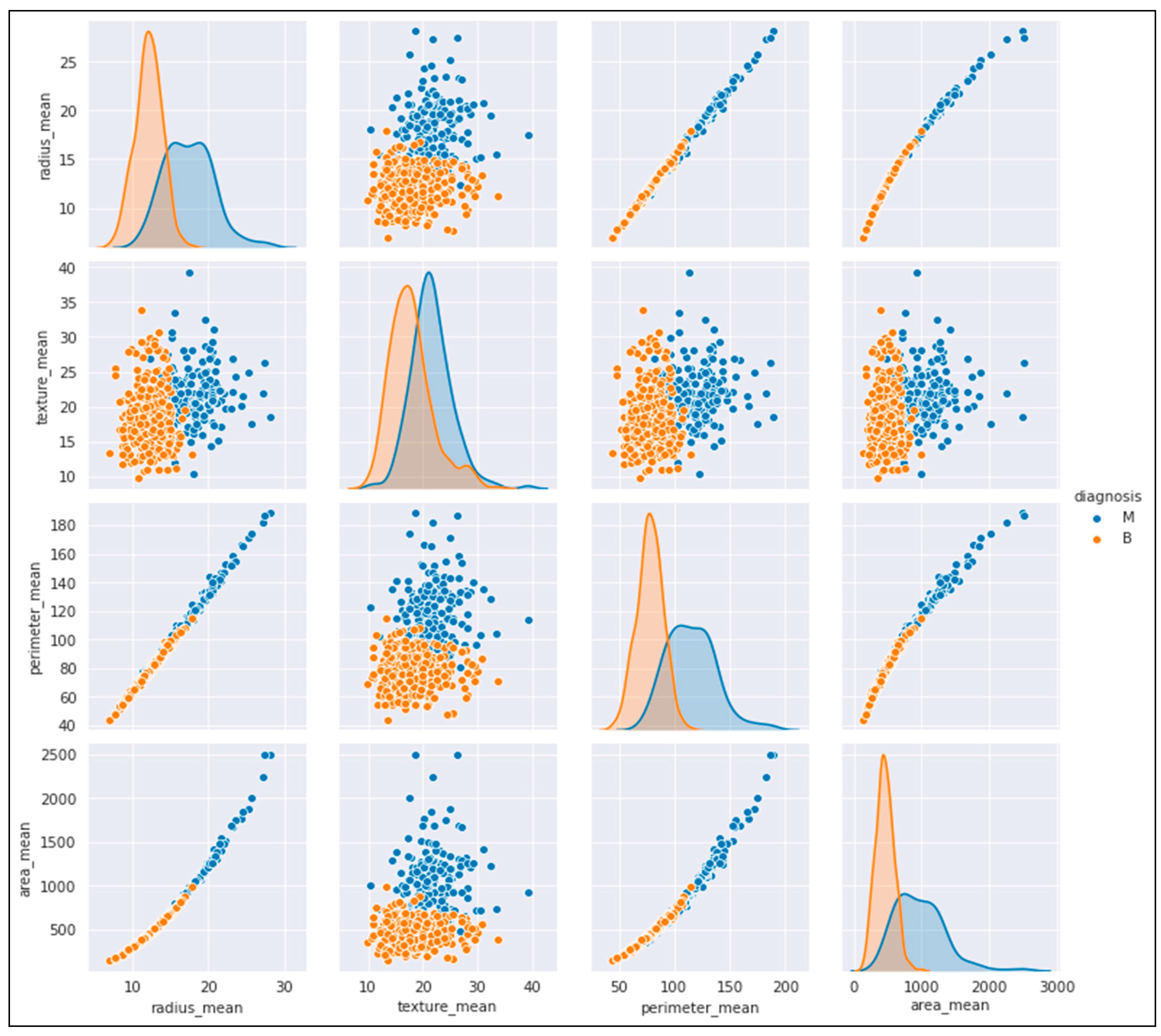
A distribution plot is a visual representation of the distribution of a sample dataset by comparing its empirical distribution with the theoretical values expected given a specific distribution. The range and distribution of a set of numerical values are shown in a distribution plot. This graph can be displayed in three different ways: with just the value points to show the distribution; with the bounding box to show the range, or with a combination of both to show the distribution and the range. Figure 2 shows the distribution plots of different features (radius_mean, texture_mean, perimeter_mean, area_mean) of the selected dataset used for this research.

When attempting to portray distribution, histograms are typically the plot type of choice. The data are divided into equal-sized intervals or classes and thus display the frequency with which certain values occur. In this way, we can obtain a rough idea of the probability distribution of the quantitative data.

3.2.2. Correlation between Features Analysis

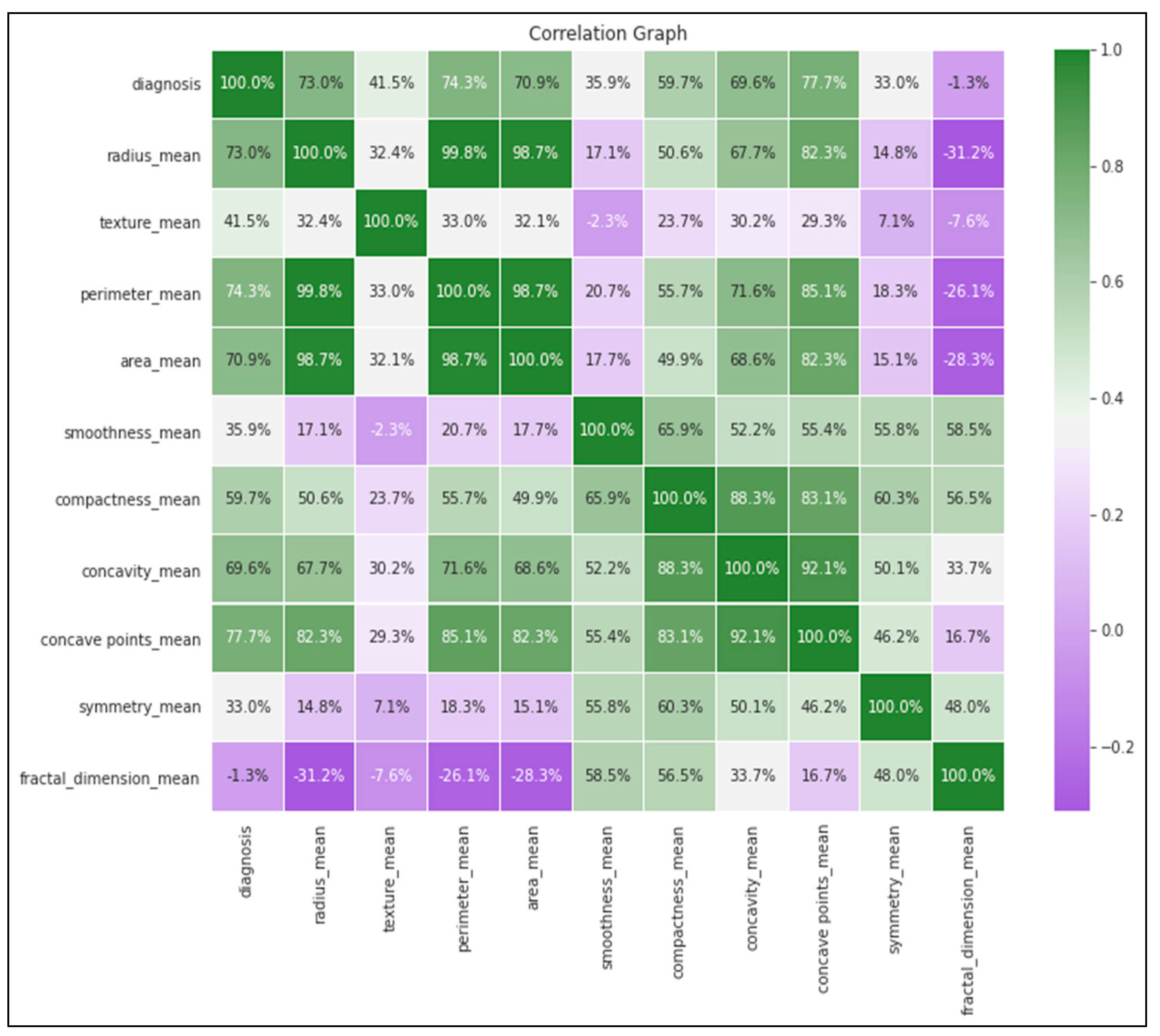
A heatmap is a graphical representation in which the values of a matrix are shown as colors. A heatmap is highly useful when trying to see the concentration of data in two dimensions of a matrix. We can find out how closely two variables are linked by performing correlation analysis on them. Calculating the correlation coefficient, which tells how much one variable changes when the other does, and vice versa is the process of correlation analysis. A linear relationship between two variables can be determined via correlation analysis. In Figure 3, each value in the dataset is represented by a different color in a two-dimensional matrix. Using a simple heatmap, a user can gain a comprehensive understanding of the data. Two-dimensional cell values that are greater than zero suggest a positive correlation between attributes, whereas values that are less than zero imply that there is a negative correlation between attributes. The lighter the color, the stronger the negative correlation, while the darker the color, the stronger the positive correlation observed in the heatmap.

The Pearson correlation coefficient, which measures the linear association between two variables, is one technique to quantify this relationship. It has a value between -1 and 1 and is calculated as follows:

• −1 is used for negative linear correlation between two features of the dataset;
• 0 is used for no linear correlation between two different features of the dataset;
• 1 is used for positive linear correlation between two different features of the dataset.

3.2.3. Feature Importance

The phrase “Feature Importance” refers to a collection of methods for assessing the relative values of various input data points in a predictive model. For regression and classification problems, which both have to do with predicting a number, it is possible to figure out scores of how important each feature is. Feature relevance ratings can be used to obtain insight into the dataset. The relative scores can be used to determine which aspects matter most to the target audience and which features matter the least. It is possible to use this as a jumping-off point to gather additional or different information. To obtain a better understanding of how the model functions, feature importance scores can be used. For the most part, the relevant results were derived using predictive models that were trained on a large sample of data. It is possible to gain a sense of how significant a model is by looking at the importance score, which shows which features are most and least crucial to the model. This form of analysis can make use of models that support this interpretation. The relevance of a feature can help enhance a prediction model. It is possible to achieve this goal by using relevance ratings to identify which features should be removed and which should be kept (highest scores). This strategy for choosing which features to use could make the problem easier to understand, speed up the modelling process (which is called “dimensionality reduction”), and possibly make the model work better. Figure 4 shows the class-level features that are important from the breast cancer Wisconsin dataset.

3.2.4. Explore Target Attribute

A particular category of an attribute is what a supervised model intends to zero in on as its target. The historical values that were used in the training of the model are stored in the target column of the training data. In the test data, the column labelled “target” contains the historical values that are used to evaluate the accuracy of the forecasts. Benign tumors are not believed to be cancerous for the following reasons: their cells appear to be close to normal; they develop slowly, and they do not infiltrate neighboring tissues or spread to other parts of the body. Malignant tumors are malignant growths, as their name suggests. In Figure 5, of 569 instances from the selected dataset, two class values, benign tumors (B) and malignant tumors (M), are distributed at 357 and 212, respectively.

3.2.5. Outlier Detection

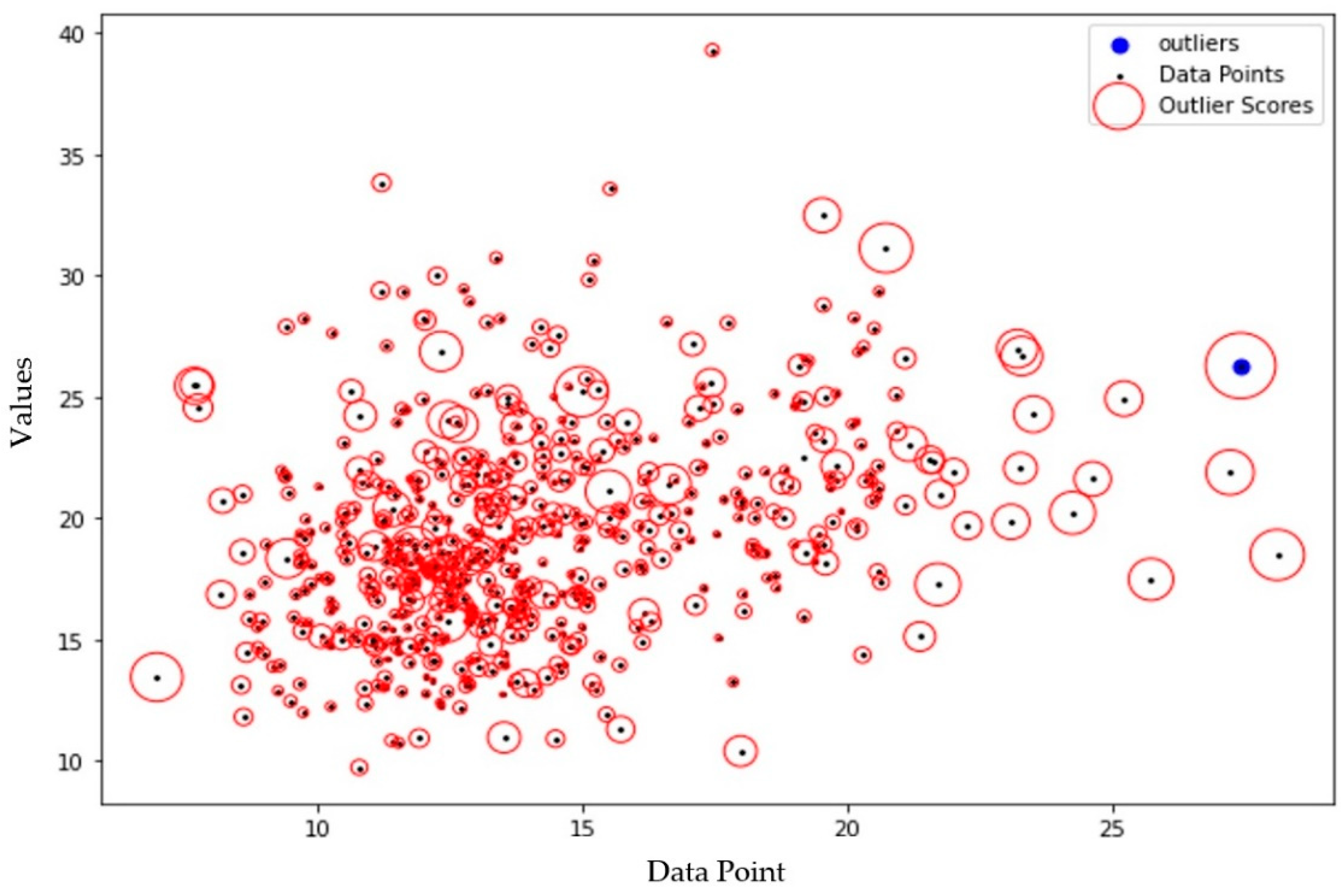
During the exploratory data analysis stage of the data science project management process, a model’s capacity to solve a business problem is contingent on how well it manages outliers. This is because managing outliers is an integral part of this stage. Data points are referred to as “outliers” when they do not appear to match the rest of the data in any way, shape, or form. The most common kind of outlier is one that is significantly removed from most of the observations or the average of the data. When we only have one or two variables, it is easy to show the data with a simple histogram or scatter plot. However, when we have a high-dimensional input feature space, this task becomes much harder. It is possible that straightforward statistical methods, such as those that rely on standard deviations or the interquartile range to find outliers, will not work in this scenario. During the process of training machine learning algorithms for predictive modelling, it may be essential to identify and eliminate any data points that are outliers. Outliers have the potential to skew statistical measurements and data distributions, which can obscure the underlying nature of the data and the relationships between the variables. It is possible to increase the fit of the data and, as a result, the accuracy of the predictions if the training data are prepared for modelling by removing outliers. Figure 6 shows the outlier detection analysis of the breast cancer Wisconsin dataset used for this study.

3.3. Classification Algorithms

In general, a classification algorithm is a function that weights the input features in such a way that the output distinguishes between one class’s positive values and the other class’s negative values. The training of the classifier is carried out to locate the weights (and functions) that provide the clearest and most precise demarcation between the two categories of data. The act of identifying, comprehending, and organizing concepts and objects into predetermined categories or “sub-populations” is the process that is referred to as classification. Machine learning systems utilize a variety of methods to classify future datasets. These algorithms are honed using pre-classified datasets. In the field of machine learning, training data are used by an algorithm to make predictions about whether new data will fit into one of the predetermined categories.

3.3.1. K-Nearest Neighbors

Traditional machine learning techniques have been extended to work with big datasets, such as those used in data mining. When it comes down to it, a large amount of training data must be used to define each data point. Each point is conceptually displayed in a high-dimensional space, where every axis in the space corresponds to a different individual variable. When evaluating a new data point, we try to find the K nearest ones. The most prevalent kind of measurement for distance is called the Euclidean distance. Euclidean distance is sometimes simply referred to as distance, as shown in Equation (1), where pi and qi are the two nearest points.

$$\mathrm{d}(\mathrm{p},\mathrm{q})=\mathrm{d}(\mathrm{q},\mathrm{p})=\sqrt{{\left({\mathrm{q}}_1-{\mathrm{p}}_1\right)}^2+{\left({\mathrm{q}}_2-{\mathrm{p}}_2\right)}^2+\cdots +{\left({\mathrm{q}}_{\mathrm{n}}-{\mathrm{p}}_{\mathrm{n}}\right)}^2)}=\sqrt{{{\displaystyle \sum }}_{\mathrm{i}=1}^{\mathrm{n}}{\left({\mathrm{q}}_{\mathrm{i}}-{\mathrm{p}}_{\mathrm{i}}\right)}^2}$$

(1)

Using the Euclidean distance measure is strongly recommended when dealing with a large volume of continuous or dense data. The Euclidean distance is the most accurate measure of proximity. The length of the line segment that joins two points is the measure of the Euclidean distance between them. This distance between two places can be calculated using the Pythagorean theorem. The L2 norm, which is also called the L2 distance, is like the Euclidean norm, but it is more general.

3.3.2. Random Forest

The random forest algorithm helps machine learning researchers with regression and classification. Ensemble learning combines multiple classifiers to handle complex problems. A random forest uses many decision trees. The random forest algorithm can be trained using bagging or bootstrap aggregation. Bagging, an ensemble of other algorithms, can improve machine learning algorithm accuracy. A random forest approach determines the outcome after considering decision tree forecasts. It calculates the average or means of all tree outputs. Increasing the forest’s tree count improves accuracy. A random forest selects random samples from a dataset to build a decision tree and make a prediction. It is considered group learning. Samples are taken till one reaches the node to calculate the probability, then divided by the total samples. When running random forests on classification data, the Gini index is used to figure out how the nodes on a decision tree branch are spread out.

$$\mathrm{Gini}\mathrm{Index}=1-{{\displaystyle \sum }}_{\mathrm{i}=1}^{\mathrm{c}}{({\mathrm{p}}_{\mathrm{i}})}^2$$

(2)

Equation (2) considers both the class and the probability when calculating the Gini value of each branch on a node. This allows one to decide which of the branches is more likely to take place. In this case, pi is going to stand for the relative frequency of the class that you are observing in the dataset, and c will stand for the total number of classes. Entropy is another tool we may use to figure out how the nodes in a decision tree branch out.

$$\mathrm{Entropy}={{\displaystyle \sum }}_{\mathrm{i}=1}^{\mathrm{c}}-{\mathrm{p}}_{\mathrm{i}}\times {\log }_2\left({\mathrm{p}}_{\mathrm{i}}\right)$$

(3)

Entropy is a method for determining how a node should branch based on the probability of a particular result by looking at all the possible branches as shown in Equation (3). Since the logarithmic function is used to figure it out, it takes a lot more calculation work to figure out than the Gini index.

3.3.3. Logistic Regression

It is one of the most extensively used machine learning techniques that fall outside the scope of the supervised learning approach. It is possible to forecast the categorical dependent variable using a specified set of independent factors. A categorical dependent variable can be predicted using logical regression. A statistical model that determines the relationship between variables and produces a yes-or-no answer. First, it compares the outcome without any predictors to the baseline outcome, and then it calculates the difference. The found variable is used as part of the equation that calculates the regression coefficient. A multilevel logistic regression model is seen in Equation (4).

$$\mathrm{logit}\left(\mathrm{Pr}\right({\mathrm{A}}_{\mathrm{ij}}=1\left)\right)={\propto }_0+{\propto }_{0_{\mathrm{j}}}+{\propto }_1{\mathrm{B}}_{1_{\mathrm{ij}}}+\cdots +{\propto }_{\mathrm{k}}{\mathrm{B}}_{{\mathrm{k}}_{\mathrm{ij}}}+{\mathsf{\beta }}_1{\mathrm{z}}_{1_{\mathrm{j}}}+\cdots +{\mathsf{\beta }}_{\mathrm{m}}{\mathrm{z}}_{{\mathrm{m}}_{\mathrm{j}}}$$

(4)

In this model, the letters A_ij stand for the binary variable, while the letters ${\mathrm{B}}_{1_{\mathrm{ij}}}$ through ${\mathrm{B}}_{{\mathrm{k}}_{\mathrm{ij}}}$ represents the k predictor or explanatory variables that were assessed for this model. In the end, we will call ${\mathrm{z}}_{1_{\mathrm{j}}}$ through ${\mathrm{z}}_{{\mathrm{m}}_{\mathrm{j}}}$ the m predictor variables that were tested on the ${\mathrm{j}}^{\mathrm{th}}$ cluster.

3.3.4. Decision Tree

Decision trees, a form of supervised machine learning, are used to divide the data indefinitely according to a particular parameter. Nodes and leaves can be used to characterize the tree in terms of their relationships to other nodes and other leaves. The leaves reflect the decisions or repercussions in their entirety. Decided nodes are where the data are split into smaller chunks. Many different algorithms, such as ID3, CART, and C4.5, are used to build a decision tree to gather the essential information to decide. Classification and regression problems can be solved using this strategy.

3.3.5. Support Vector Machine

Classification and regression can both be performed using a support vector machine (SVM), which is a supervised machine learning technique. Even though we also cover regression issues, its utilization is more suited to classification tasks than regression tasks themselves. The SVM algorithm can help with analyzing data points in an N-dimensional space. The SVM approach is used to find a hyperplane in a space of N dimensions where the data points may be classified in a way that is distinct from one another. Hyperplanes can be selected from a wide range of options to distinguish between the two types of data points. We have assigned ourselves the task of finding a plane with the biggest margin, or the maximum distance between data points from both classes. To make it easier to classify the next set of data, some reinforcement is given when the margin distance is as large as it can be. When using the SVM approach, we are trying to obtain hyperplane and data points as far apart as feasible. One way to increase the margin is to use a loss function known as hinge loss.

3.3.6. AdaBoost Classifier

The AdaBoost algorithm is part of a boost strategy known as “Adaptive Boosting” in which boosts are redistributed for each instance in adaptive boosting, with higher weights applied to instances that were incorrectly classified. To minimize bias and variation, boosting is employed in supervised learning. It is built on the idea of incremental improvement through time. Except for the first, all subsequent students are built upon the foundation of their predecessors. As a result, weak students become strong ones. With a few exceptions, the AdaBoost algorithm is based on the same ideas as the boosting method. In each round of the AdaBoost algorithm, a misclassified instance is given more weight. This is done by combining the weak classifier with the strong classifier to improve classification accuracy.

$${\mathrm{E}}_{\mathrm{t}}={{\displaystyle \sum }}_{\mathrm{i}}\mathrm{E}\left[{\mathrm{F}}_{t-1}\left({\mathrm{x}}_{\mathrm{i}}\right)+{\alpha }_t\mathrm{h}\left({\mathrm{x}}_{\mathrm{i}}\right)\right]$$

(5)

In Equation (5), E_t demonstrates how a weak learner uses an object x, h(x_i) is assumed, and the coefficient for each weak learner is α_t in a way that minimizes the total amount of training errors.

3.3.7. Gradient Boosting Classifier

In machine learning, gradient boosting is a type of boosting. When combined with previous models, it is assumed that the overall prediction error is minimized. The fundamental idea is to describe the desired results for this new model to limit the risk of making mistakes. Regressors can be used to forecast both continuous and categorical target variables using the gradient boosting method (as a classifier). A mean square error (MSE) is the cost function for regressors, while a log loss is the cost function for classifiers.

3.3.8. Stochastic Gradient Boosting Classifier

The stochastic gradient boosting (SGB) method proposed by Friedman, J. H. [29] combines bagging and boosting techniques. By weighing the ensemble members of all trees, this ensemble learning technique, which combines boosting and decision trees, generates a forecast. The new model is constructed during the iteration in the gradient descent direction of the prior tree’s loss function. The goal of SGB is to train the classification function to reduce the loss function between it and the real function. The classification issue is discussed in the prediction of construction accidents. SGB is the name given to this variant of boosting. A random subsample of training data is taken from the entire training dataset for each iteration. The whole sample is then thrown away, and the randomly chosen subsample is used to fit the base learner.

3.3.9. CatBoost Classifier

CatBoost is a machine learning technique created by Yandex, N.V. [30] that uses a boosted decision tree. There are many similarities between this method and other gradient-boosted algorithms such as XGBoost, but it also includes categorical variable support out of the box and has a greater level of accuracy without modifying parameters. CatBoost uses a novel gradient-boosting approach to reduce overfitting when building models. CatBoost is 13–16 times faster at learning and making predictions than other algorithms since it takes advantage of distributed GPUs.

3.3.10. XGBoost Classifier

XGBoost is a machine-learning technique that uses structured and tabular data to classify objects. XGBoost is a gradient-boosted decision tree solution that is optimized for speed. A technique known as XGBoost, which stands for “extreme gradient boost” has been developed. There are a lot of different parts to this machine learning process. Extensive and complex datasets can be handled by XGBoost. XGBoost is a method for ensemble modelling. XGBoost is an approach to collective learning. One machine learning model’s output is not always enough to decide. Using a systematic approach, ensemble learning combines the predictive capacities of multiple students. As a result, the output of many models is combined into a single model. Models can be treated as classifiers or regressors in the SciKit-learn framework using XGBoost’s wrapper class. The SciKit-learn package can be used in full with XGBoost models. The XGBoost model used for classification is called XGBClassifier. Afterward, we can use our training data to make it work.

3.4. Performance Metrics

Evaluating a machine learning model’s performance is one of the most important steps in the process of creating an efficient model. There are a variety of metrics that are utilized to evaluate the quality of the model, and these measurements are referred to as either performance metrics or evaluation metrics. With the use of these performance indicators, we can evaluate how successfully our model worked with the data that were provided. We can improve the performance of the model by adjusting the hyper-parameters. When it comes to evaluation, the tasks of regression and classification each use their unique metrics. In this subsection, we are going to talk about the metrics that are utilized for classification and regression tasks. The KPIs that are used to compare how well the proposed solution works to how well the existing solutions work are discussed below.

3.4.1. Accuracy

The accuracy of a machine learning algorithm is one way to measure how often it is successful in classifying a data point correctly. Accuracy refers to the percentage of data points that were correctly predicted out of all the data points. Accuracy is calculated by dividing the total number of true positives and true negatives samples by the total number of true positive, true negative, false positive, and false negative samples. Data that the algorithm correctly detects as true or untrue are “true positive” or “true negative” data points. A false positive or false negative, on the other hand, is a data point that the algorithm incorrectly classified.

$$\mathrm{Accuracy}=\frac{\left(\mathrm{tp}+\mathrm{tn}\right)}{\left(\mathrm{tp}+\mathrm{fp}+\mathrm{fn}+\mathrm{tn}\right)}$$

(6)

In Equation (6), tp = true positive values, tn = true negative, fp = false positive, and fn = false negative.

3.4.2. Precision

In mathematics, precision is calculated by dividing the total number of true positive samples by the total number of true positive and false positive samples. High precision results in fewer false positives. The following equation is used to arrive at the result.

$$\mathrm{Precision}=\left(\mathrm{tp}\right)/\left(\mathrm{tp}+\mathrm{fp}\right)$$

(7)

3.4.3. Recall

Recall is calculated by dividing the total number of true positive samples by the total number of true positive and false negative samples. The recall measure is used to assess the model’s ability to identify positive samples. There are more positive samples when the recall is higher. Equation (8) can be used to express the recall rate:

$$\mathrm{Recall}=\left(\mathrm{tp}\right)/\left(\mathrm{tp}+\mathrm{fn}\right)$$

(8)

The occurrence of the event is often referred to as the event’s sensitivity.

3.4.4. F-Measure

To arrive at the F-measure, precision and recall are given equal weight in the harmonic mean. If you are comparing models, it is helpful to know how accurate your model is by utilizing a single score that takes into consideration both precision and recall. Because it is based on average precision and recall, it considers both true positives and false negatives.

$$\mathrm{F}1\mathrm{Score}=\frac{\left(2\times (\mathrm{Recall}\times \mathrm{Precision}\right))}{\left(\mathrm{Recall}+\mathrm{Precision}\right)}$$

(9)

The combined measurements, which benefit from enhanced sensitivity, are presented in Equation (9). Every machine learning model tries to generalize well for data that it has not seen before or new data, and performance metrics are used to help determine how well the model generalizes for the new dataset. In the field of machine learning, every assignment or challenge is broken down into classification and regression.

4. Proposed Optimized Stacking Ensemble Learning (OSEL) Model

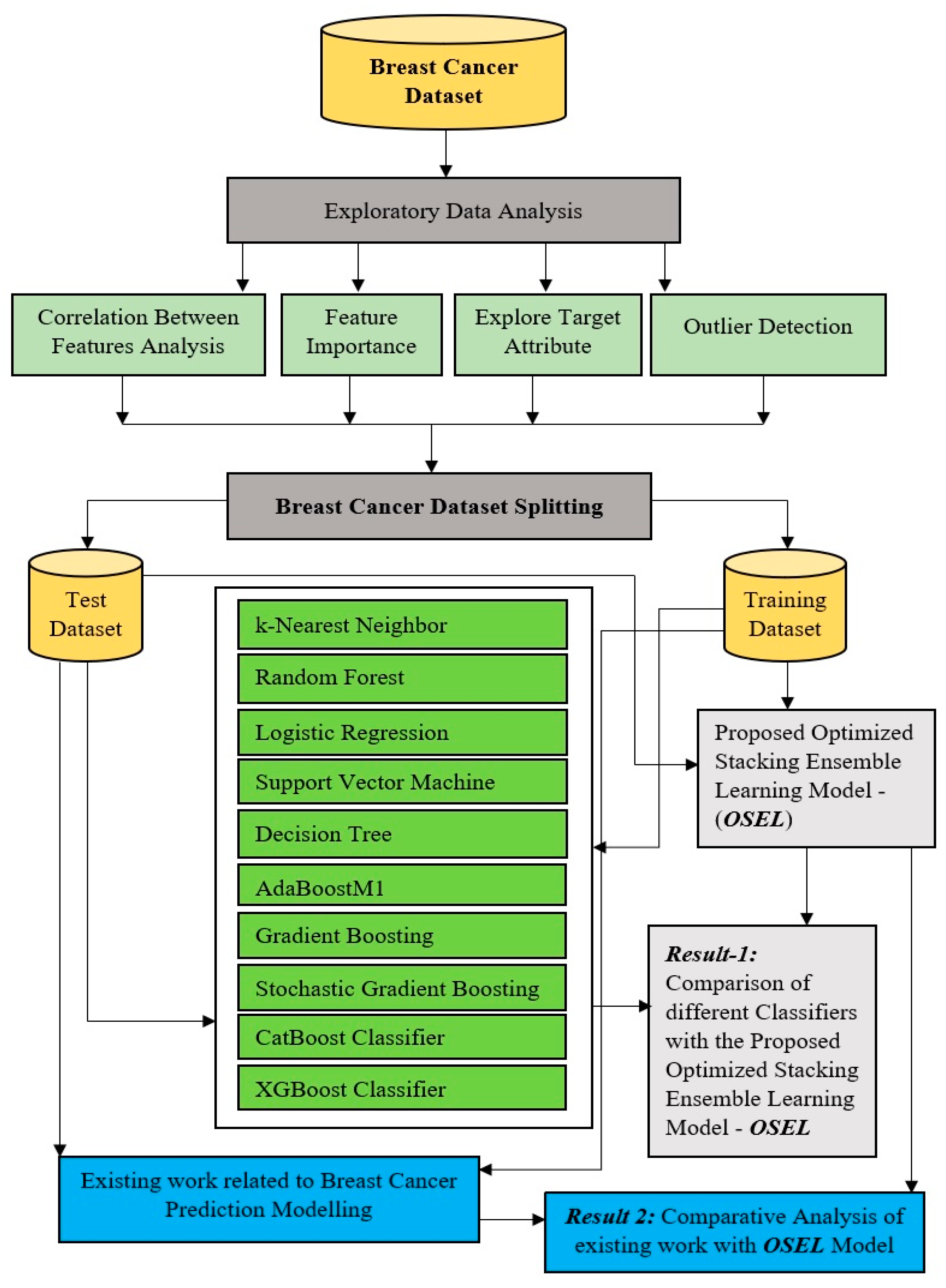
Building predictive models is an iterative process that begins with a hypothesis and continues until a useful outcome is achieved. Predictive models may require statistical analysis, data mining, or data visualization technologies. In Figure 7, an approach to machine learning, including any method of deep learning, can function as a base classifier for the OSEL model. The level of difference between the different base classifiers is a large part of how the base classifiers are chosen.

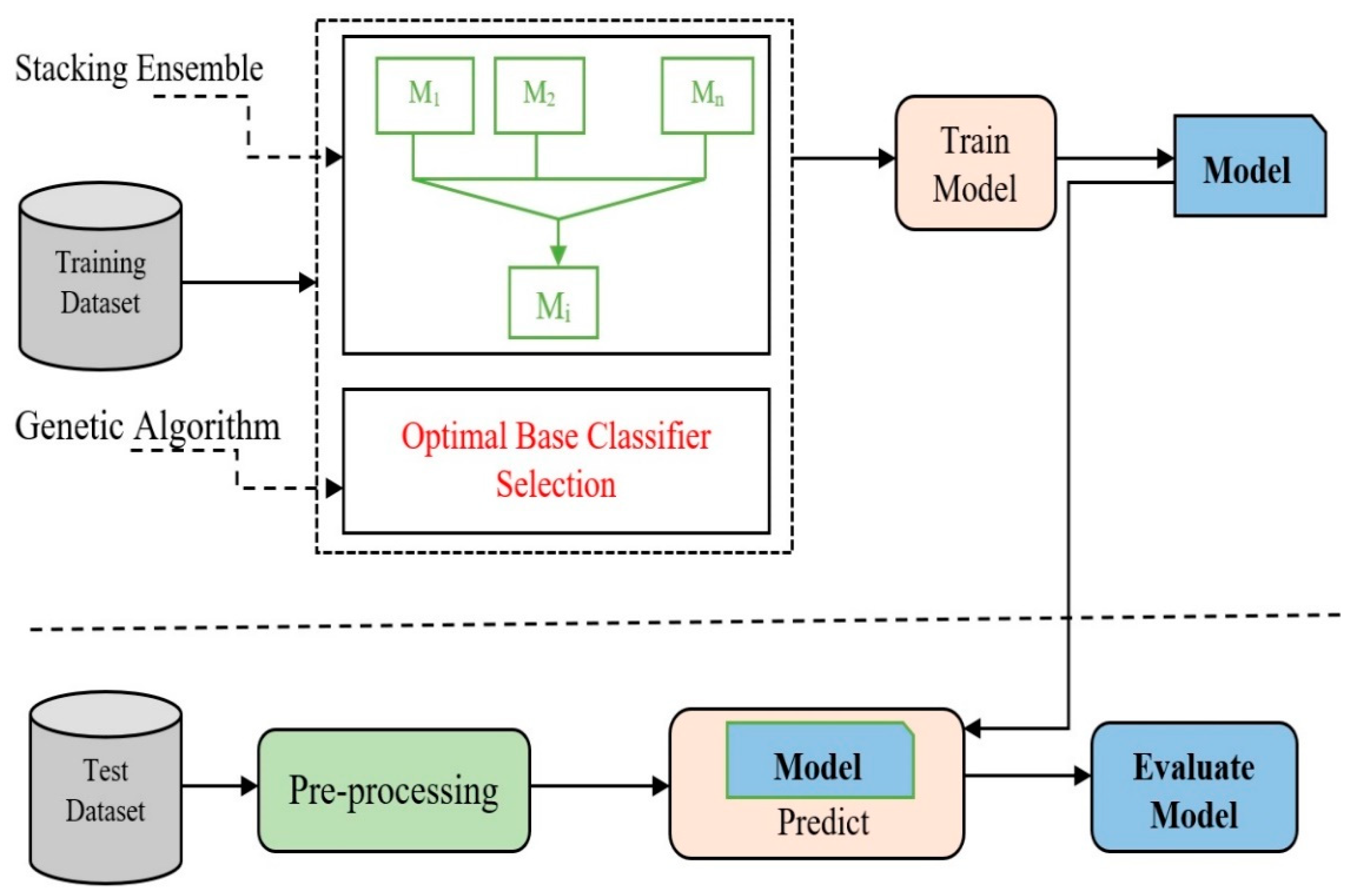
For this model, we consider the following cutting-edge classifiers as possible starting points: k-nearest neighbor; random forest; logistic regression; support vector machine; decision tree; AdaBoostM1; gradient boosting; stochastic gradient boosting; and CatBoost. These classifiers represent cutting-edge classification technology. Figure 7 shows how the proposed model was built using the previously mentioned stacking ensemble model and the genetic algorithm. After stacking up several base classifiers, the OSEL model uses a genetic algorithm to figure out the best way to use them together.

An architectural framework for stacking ensemble learning is given in Figure 8. For the meta-classifier layer, a new feature matrix is generated from the training set, which is used to train the meta-classifier layers. When making a final prediction, the meta-classifier layer chooses which classifier to utilize. One of the most important steps is picking the best possible combination of basic classifiers.

The genetic algorithm is an example of a heuristic optimization technique. The genetic algorithm is commonly used to search input spaces. Enumerating all items is not necessary for the evolutionary algorithm, which is equivalent to using brute force, to achieve its goal of giving the most efficient answer possible. It has the advantage of avoiding performance concerns that can be caused by many queries. In most cases, a genetic algorithm is used to simulate the process of naturalization. The adoption of the probabilistic optimization method allows the evolutionary algorithm to automatically get guidance on the optimal search space. After the optimization is complete, we do not have to worry about setting up the rules again.

Algorithm for Selecting Optimized Base Classifier for Stacking

Our proposed optimized base classifier for stacking uses different base classifiers and meta classifiers that are discussed in this section. Here, f, b, and d are feature vector sets which are generated from the dataset; b represents the base classifiers set which is implemented on different feature sets and d represents the trained base classifiers set. The n input features vector is represented by f = [f₁, f₂..., f_n]. Let b = [b₁, b₂..., b_k] represents the k-train base classifiers. Finally, let d = [d₁, d₂…, d_m] represent the output of the m-train base classifiers.

The following is an example of what the i^th trained base classifier came up with:

$${\mathrm{d}}_{\mathrm{i}}=\mathrm{b}\left({\mathrm{f}}_{\mathrm{i}}\right)$$

(10)

Among the basis classifiers, the meta classifier m_c is chosen from the b vector, thus the final output p = [p₁, p₂, …, p_n] is represented as follows:

p_i = m_c(d_i)

(11)

The actual value of the dataset sample is represented by y = [y₁, y_2, …, y_n], and we make use of the trained base classifiers having the highest accuracy in making predictions. Trained base classifiers with a greater prediction accuracy are more effective. It is possible, using the OSEL model, to produce k additional meta-classifiers as well as the meta-classifier. The best base classifier was chosen by applying the following criteria:

$$\min \mathrm{j}(\mathsf{\theta })=\frac{1}{\mathrm{m}}{{\displaystyle \sum }}_{\mathrm{i}=1}^{\mathrm{m}}{(\parallel {\mathrm{y}}_{\mathrm{i}}-{\mathrm{p}}_{\mathrm{i}}\parallel )}^{2}s.t\{\begin{array}{c}1\le i\le m\\ {\mathrm{b}}_{\mathrm{i}} \in b\\ {\mathrm{m}}_{\mathrm{c}} \in b\end{array}$$

(12)

where y_i represents the actual value and p_i represents the predicted value.

5. Implementation of the Proposed OSEL Model

An ensemble learning approach integrates numerous independent learning algorithms, and its performance is often either superior to or comparable to that of a single base classifier. As a result, it has grown in popularity and is proving to be an efficient strategy in the field of machine learning. There are fundamental problems that need to be fixed with the ensemble learning approaches. The first problem is figuring out how to mix base classifiers that are “excellent” and “different.” Accuracy, recall, precision, and F1 score are four prominent measures that are utilized while dealing with categorization issues. In the first place, accuracy can judge the overall judgement skill of the categorization work. The percentage of the actual sample that can be predicted can be calculated using recall. Finding the harmonic mean of the precision score and the recall score is the first step in calculating the F1 score. For the dataset of breast cancer cases in Wisconsin presented in

Table 2. Accuracy by machine learning algorithms.

Classifier Model	Accuracy	Precision	Recall	F-Measure
k-Nearest Neighbor (k-NN)	95.32%	0.97	0.91	0.94
Random Forest (RF)	95.90%	0.97	0.91	0.94
Logistic Regression (LR)	97.66%	0.98	0.95	0.97
Support Vector Machine (SVM)	97.66%	0.98	0.95	0.97
Decision Tree (DT)	91.22%	0.88	0.89	0.89
Proposed OSEL Model	99.45%	0.99	0.98	0.99

, a variety of categorization approaches were evaluated. Based on the different findings and a close look at them, the suggested ensemble model was built on top of the learning models that were chosen. We compared the OSEL model’s performance to other state-of-the-art classification algorithms to demonstrate its efficacy. The algorithms are as follows: k-nearest neighbor, random forest, logistic regression, support vector machine, decision tree, AdaBoostM1, gradient boosting, stochastic gradient boosting, XGBoost classifier, and CatBoost.

Table 2 summarizes the outcomes of implementing a variety of machine learning algorithms that use k-fold cross-validation. Every dataset attribute was considered in the development of these algorithms. We also considered the accuracy of the system’s recall, precision, and F-measure in our evaluations. When compared to other well-known classifiers, our suggested OSEL model does better in terms of recall, precision, and F-measure.

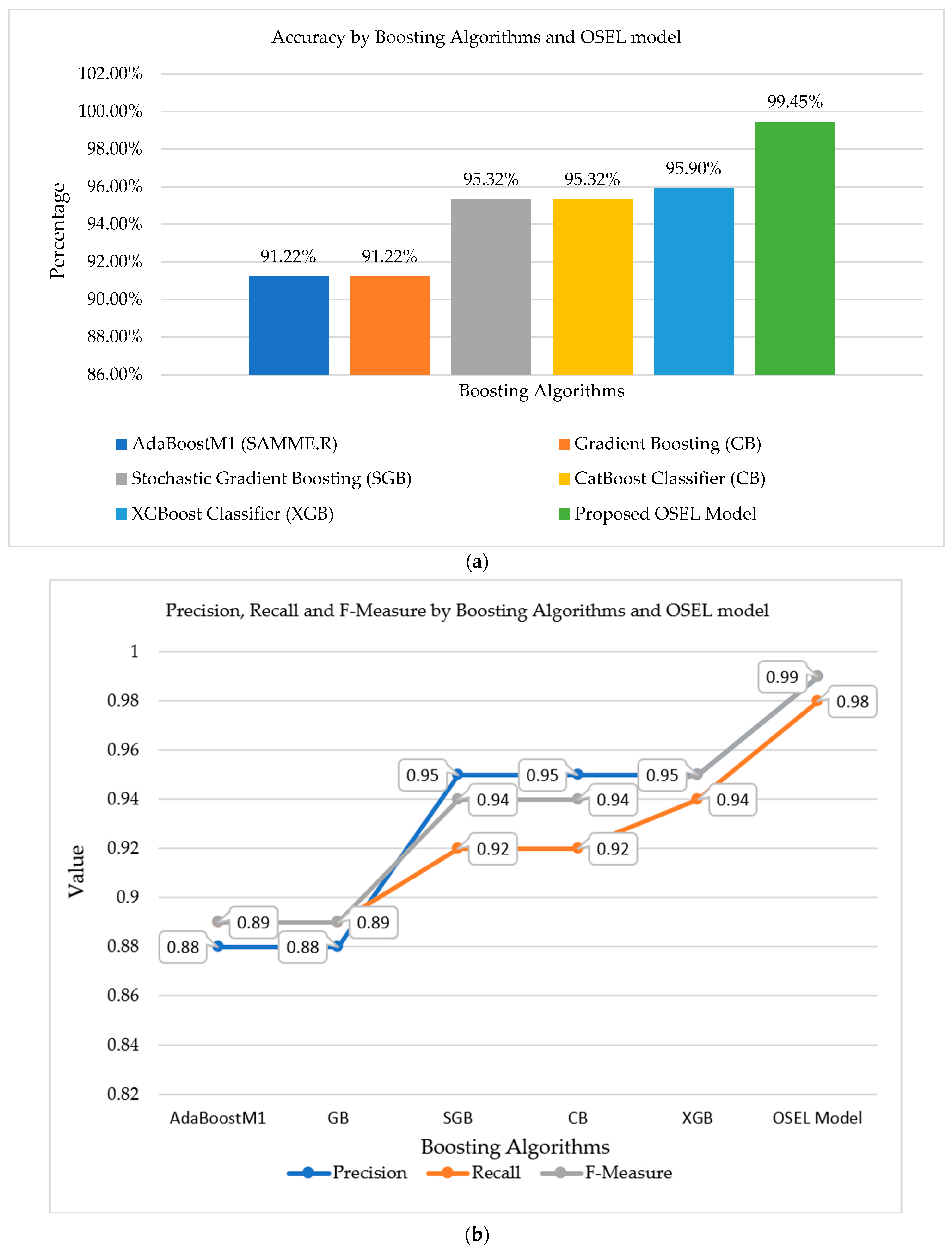
When compared to existing models’ performance metrics, the results of the suggested model reveal that it has shown better results. A diagrammatic representation of all the classifiers used on a given dataset is shown in Figure 9. With a maximum of 99.45%, the proposed OSEL model is shown in Figure 9. The decision tree algorithm has the lowest accuracy (91.22%). In

Table 3. Accuracy by boosting algorithms on breast cancer Wisconsin dataset.

Classifier Model	Accuracy	Precision	Recall	F-Measure
AdaBoostM1 (SAMME.R)	91.22%	0.88	0.89	0.89
Gradient Boosting (GB)	91.22%	0.88	0.89	0.89
Stochastic Gradient Boosting (SGB)	95.32%	0.95	0.92	0.94
CatBoost Classifier (CB)	95.32%	0.95	0.92	0.94
XGBoost Classifier (XGB)	95.90%	0.95	0.94	0.95
Proposed OSEL Model	99.45%	0.99	0.98	0.99

, the implementation results of five different boosting algorithms along with the proposed OSEL model are mentioned. In boosting algorithms, only CatBoost, XGBoost, and stochastic gradient boosting classifiers achieved maximum accuracies of 95.32%, 95.90%, and 95.32%, respectively. However, the proposed model achieved a maximum accuracy of up to 99.45% as compared to other well-known boosting classifiers.

A graphical representation of all the classifiers applied to the specified dataset is shown in Figure 10. The proposed classification model (OSEL) had a maximum accuracy of 99.45%, as shown in Figure 10. AdaBoostM1 (SAMME.R) and gradient boosting (GB) have the lowest accuracy, up to 91.22%, whereas other boosting algorithms reached accuracies of up to 95.9%.

The suggested model’s results clearly show that it outperforms the existing model in terms of performance parameters. Figure 10 depicts a graphical representation of all the classifiers used on the chosen dataset. According to Figure 10, the proposed OSEL model had a maximum accuracy of up to 99.45%. The AdaBoostM1 (SAMME.R) algorithm has the lowest accuracy of 91.22%.

6. Comparison of OSEL Model with Existing Models

In the section below,

Table 4. Comparison of the proposed OSEL model with existing models.

Authors/Ref. No.	Machine Learning Algorithm Used	Accuracy
Nguyen, Q. H. et al. [31]	Feature selection and ensemble voting	98.00%
Osman, A. H. et al. [32]	Ensemble learning using Radial Based Function Neural Network models (RBFNN)	97.00%
Nahato, K. B. et al. [33]	Backpropagation neural network	98.60%
Chen, H. L. et al. [34]	An SVM classifier with rough set-based feature selection (RS-SVM)	96.72%
Kumari, M. et al. [35]	k-NN classification algorithm	99.28%
Dumitru, D. et al. [36]	Naïve Bayesian classification	74.24%
Shaikh, T. A. et al. [37]	Dimensionality reduction and SVM	97.91%
Alickovic, E. et al. [38]	Normalized multi-layer perceptron neural network	99.27%
Kaushik, D. et al. [39]	Ensemble learning via MLP, RF and RT	83.50%
Proposed OSEL Model		99.45%

displays the results of numerous models applied to the same Wisconsin breast cancer dataset by various authors. The proposed OSEL model is significantly more effective at predicting breast cancer in patients. Although a great deal of research has been conducted on the topic, only a small subset of recent contributions was selected for comparison and discussion in this article. As well as varying degrees of precision, each model also has its unique benefits and drawbacks. Therefore, in this investigation, we compare various classification models by using a wide range of classification algorithms, using accuracy as a metric. These elements are considered during the production process. Classifier accuracy, model type, and construction technique are all summarized in Table 4.

According to the scaling and main component analyses of Nguyen, Q. H. et al. [31], the ensemble voting technique is effective as a breast cancer prediction model. Subsequently, the random forest method is used to construct the reference model. After performing operations such as principal component analysis and feature scaling on the data, several models are trained and evaluated. The results of the cross-validation show that our model is reliable. The ensemble-voting classifier, SVM tuning, logistics regression, and AdaBoost models were the only ones that reached a minimum of 98% accuracy.

The RBF neural network (RBFNN) was developed by Osman, A. H. et al. [32], and the properties of the ensemble were incorporated into it. When the accuracy of the proposed method was compared to that of other breast cancer diagnosis methods, such as logistic regression, k-NN, SVM, decision tree, CNN, and naïve Bayes, before and after using ensemble boosting, the proposed method was found to have a higher degree of accuracy than the other methods. Based on a limited set of clinical parameters, they developed a classifier that can determine whether a disease is present. Nahato, K. B. et al. [33] proposed a rough set indiscernibility relation approach with a backpropagation neural network (RS-BPNN). On the dataset containing breast cancer cases, the suggested technique achieved an accuracy of 98.6%. The suggested system delivers a powerful way to classify clinical datasets that can be used to classify them.

The RS-BPNN approach is employed by Chen, H. L. et al. [34] to determine the approximate indistinctness of sets. Breast cancer is detected with 98.6% accuracy. This strategy also works well for categorizing cases of breast cancer. The RS reduction method can be used with the SVM, which is used in the suggested method (RS-SVM), to improve diagnostic accuracy even more. The Wisconsin breast cancer dataset is used to test the RS-SVM’s accuracy, sensitivity, specificity, confusion matrix, and receiver operating characteristic (ROC) curves. RS-SVM may be able to accurately categorize things up to 696.72% based on the results of the tests.

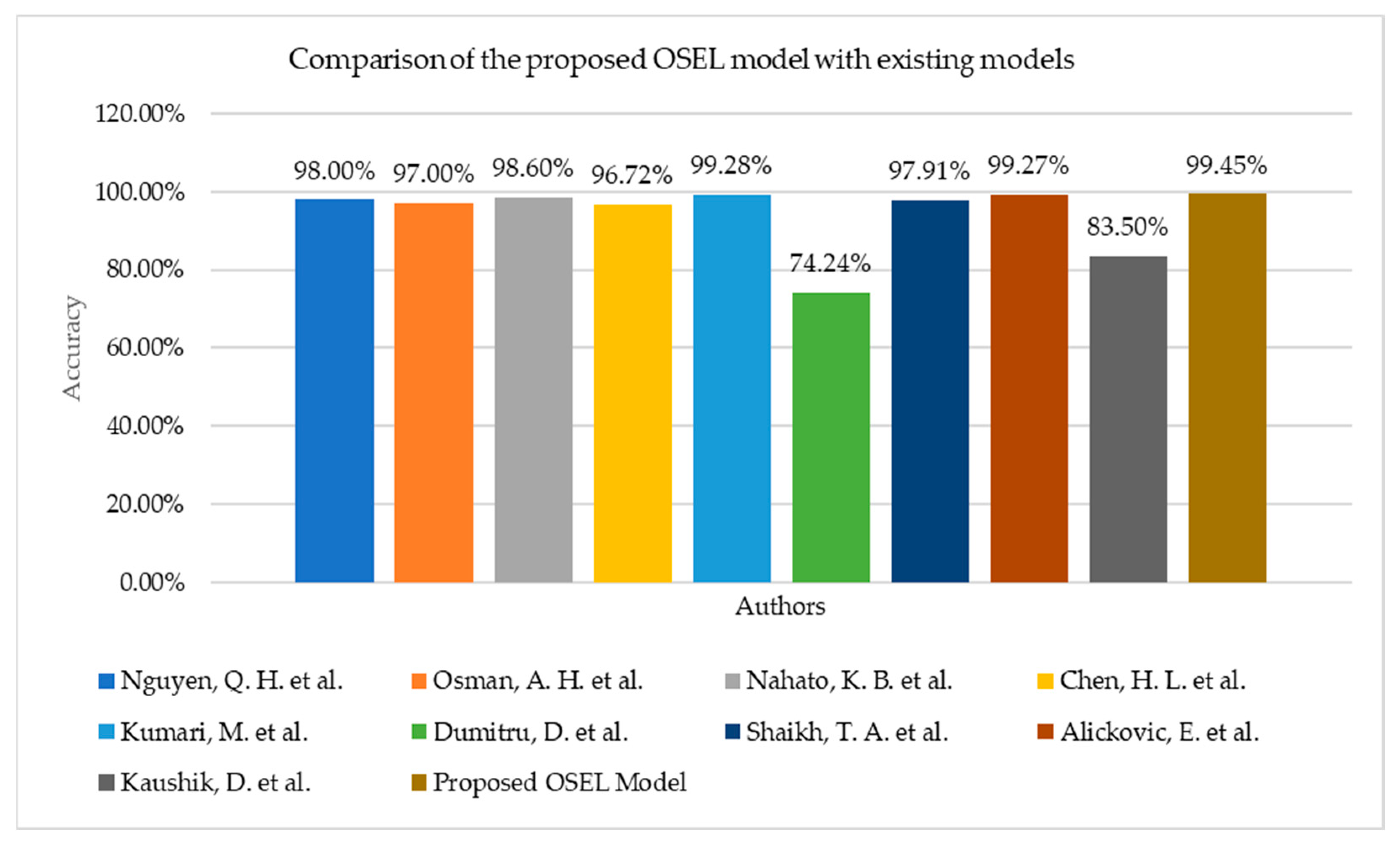
Kumari, M. et al. [35] developed a prediction algorithm for early breast cancer detection by analyzing a small subset of clinical dataset attributes. The potential of the suggested approach is evaluated by contrasting the true and anticipated classification accuracy. The results show that the goal of 99.28% accuracy in categorization was met. Dumitru, D. et al. [36] examined the potential use of the naïve Bayesian classification approach as an accurate aid in the computer-aided diagnosis of such events using the widely-used Wisconsin prognostic breast cancer dataset. The outcomes proved that when comparing computing effort and speed, the naïve Bayes classifier is the most effective machine learning method. As shown by the results, the best classification accuracy (74.24%) was achieved. Figure 11 shows the graphical representation of different models implemented by authors on the same Wisconsin breast cancer dataset with their achieved accuracy. Shaikh, T. A. et al. [37] used Weka’s WrapperSubsetEval dimensionality reduction algorithm on the Wisconsin breast cancer dataset to reduce the dataset’s size. It was found that the naïve Bayes, J48, k-NN, and SVM models had raised their accuracy from 97.91% in the case of the Wisconsin dataset to 99.97% in the closing tests.

Alickovic, E. et al. [38] used a normalized multi-layer perceptron neural network to design a model for accurately classifying breast cancer. The results reveal a level of accuracy of up to 99.27% based on the findings. This study has a lot of promise when compared to previous ones that used artificial neural networks. To predict the outcome of a biopsy based on attributes gleaned from the dataset, Kaushik, D. et al. [39] recommended employing a data mining technique based on an ensemble of classifiers. According to the results of this investigation, the accuracy of the findings is 83.5%. With an F1-score of 0.914 and 0.974, respectively, Saxena, A. et al. [40] compared the performance of AlexNet and MobileNet. They concluded that the latter deep learning approach performs better in classifying the ultrasound images of breast tissues in benign and malignant cancer types. According to Pathak, P. et al. [41], there are two types of approaches utilized in computer-aided design (CAD) systems: the traditional technique and the artificial intelligence approach. Preprocessing, segmentation, feature extraction, and classification are only a few of the fundamental phases in image processing that are covered by the traditional method. Mangal, A. et al. [42] used convolutional and deep learning networks for diagnostics that are covered under the AI methodology. The power of machine learning classifiers was used in this study to predict breast cancer. For a common dataset, Jain, V. et al. [43] implemented three machine learning classifiers—LR, k-NN, and DT—that are used, and the prediction accuracy of each is measured. According to the outcomes obtained by Lahoura, V. et al. [44] using the Wisconsin diagnostic breast cancer (WBCD) dataset, the cloud-based extreme learning machine (ELM) methodology performs better than competing methods. When comparing standalone and cloud settings, it was discovered that ELM performed well in both cases. Two machine learning models, SVM and RF, are used to evaluate the efficacy of these feature sets. The hog features perform significantly better on these models. With an F1 score of 0.92, the SVM model trained with the hog feature set performs better than the random forest model.

The proposed approach meets the need for a 99.45% accurate optimization model for predicting breast cancer in patients. Figure 11 depicts a graphical representation of the various models and the accuracy obtained, although the proposed model in this study delivers the highest accuracy when compared to another model. Classification models that employed only one classification method in their model performed worse than those that used a combination of several classifications to generate a model. Kumari, M. et al. [35] and Alickovic, E. et al. [38] obtained 99.28% and 99.27% accuracy, respectively. To obtain the highest accuracy, the authors used hybrid classification algorithms.

7. Conclusions

Early detection is crucial because breast cancer is one of the leading causes of mortality in women. Early breast cancer tumor detection can be enhanced with the use of advanced machine learning classifiers. It is common knowledge that the success of improving a model’s predictive performance is dependent on a variety of model variables. An ensemble learning approach integrates numerous independent learning algorithms, and its performance is often either superior to or comparable to that of a single base classifier. As a result, it has grown in popularity and is proving to be an efficient strategy in the field of machine learning. One of the most important problems that need to be fixed concerns ensemble learning approaches. The problem is figuring out how to mix base classifiers that are both “excellent” and “different”. As a solution to these problems, we suggest using a novel model called the OSEL model. The OSEL model incorporates optimization models to determine the most effective combination of base classifiers. We employ the accuracy of the classifiers as the fitness function, and the genetic algorithm is the technique that we use for OSEL’s optimization. The “white box” that is created by stacking allows for a variety of different combinations. The genetic algorithm constantly makes small adjustments to the meta-classifier combination that is stored in the “white box” to achieve the best possible performance. When measured against the other 10 state-of-the-art classification methods created by a variety of authors, OSEL achieves the best or equivalent results in terms of accuracy, recall, and F1 score. Because of this, we have reason to think that OSEL may be a good way to solve classification problems. Although the OSEL performs well when it comes to classification in this work, there is still potential for improvement. OSEL does not consider the best possible choice of base-classifier hyper-parameters for each base-classifier section that is utilized in the ensemble in the work that has been done up until this point. This model was made for the specific purpose of determining whether a patient’s tumors were benign or malignant. The microscopic classification of abnormalities is a promising area for further study. Soon, complicated characteristics can be handled using a multilayered neural network design.

Further research can be carried out to determine their proportionality, and appropriate optimization strategies can be designed for improved future performance. Recent studies in relevant engineering fields, using automatic detection of Alzheimer’s disease progression [45], centralized convolutional neural network (CNN)-based dual deep Q-learning (DDQN) [46], two-tier framework based on GoogLeNet and YOLOv3 [47], feature extraction-based machine learning models [48], fuzzy convolutional neural networks [49], hybrid SFNet models [50], and intuitionistic-based segmentation models [51] can provide insight if used in related ensemble learning approaches research. There is also room to explore other recent methods [52,53].

References

1. Breast Cancer. Available online: https://www.who.int/news-room/fact-sheets/detail/breast-cancer (accessed on 9 November 2021).
2. Mao, N.; Yin, P.; Wang, Q.; Liu, M.; Dong, J.; Zhang, X.; Hong, N. Added value of radiomics on mammography for breast cancer diagnosis: A feasibility study. J. Am. Coll. Radiol. 2019, 16, 485–491. [Google Scholar] [CrossRef] [PubMed]
3. Wang, H.; Feng, J.; Bu, Q.; Liu, F.; Zhang, M.; Ren, Y.; Lv, Y. Breast mass detection in digital mammogram based on gestalt psychology. J. Healthc. Eng. 2018, 2018, 4015613. [Google Scholar] [CrossRef] [PubMed] [Green Version]
4. Valvano, G.; Santini, G.; Martini, N.; Ripoli, A.; Iacconi, C.; Chiappino, D.; Latta, D.D. Convolutional neural networks for the segmentation of microcalcification in mammography imaging. J. Healthc. Eng. 2019, 2019, 9360941. [Google Scholar] [CrossRef] [PubMed]
5. Devi, R.D.H.; Devi, M.I. Outlier detection algorithm combined with decision tree classifier for early diagnosis of breast cancer. Int. J. Adv. Eng. Technol. 2016, 12, 93–98. [Google Scholar]
6. Khan, S.; Islam, N.; Jan, Z.; Din, I.U.; Rodrigues, J.J.C. A novel deep learning-based framework for the detection and classification of breast cancer using transfer learning. Pattern Recognit. Lett. 2019, 125, 1–6. [Google Scholar] [CrossRef]
7. Huang, Q.; Chen, Y.; Liu, L.; Tao, D.; Li, X. On combining bi-clustering mining and AdaBoost for breast tumour classification. IEEE Trans. Knowl. Data Eng. 2019, 32, 728–738. [Google Scholar] [CrossRef]
8. Kharya, S.; Soni, S. Weighted naive Bayes classifier: A predictive model for breast cancer detection. Int. J. Comput. Appl. 2016, 133, 32–37. [Google Scholar] [CrossRef]
9. Chaurasia, V.; Pal, S.; Tiwari, B.B. Prediction of benign and malignant breast cancer using data mining techniques. J. Algorithms Comput. Technol. 2018, 12, 119–126. [Google Scholar] [CrossRef] [Green Version]
10. Verma, D.; Mishra, N. Analysis and prediction of breast cancer and diabetes disease datasets using data mining classification techniques. In Proceedings of the 2017 International Conference on Intelligent Sustainable Systems (ICISS), Palladam, India, 7–8 December 2017; IEEE: New York, NY, USA, 2017; pp. 533–538. [Google Scholar]
11. Ojha, U.; Goel, S. A study on prediction of breast cancer recurrence using data mining techniques. In Proceedings of the 2017 7th International Conference on Cloud Computing, Data Science & Engineering-Confluence, Noida, India, 12–13 January 2017; IEEE: New York, NY, USA, 2017; pp. 527–530. [Google Scholar]
12. Kumar, V.; Mishra, B.K.; Mazzara, M.; Thanh, D.N.; Verma, A. Prediction of malignant and benign breast cancer: A data mining approach in healthcare applications. In Advances in Data Science and Management; Springer: Singapore, 2020; pp. 435–442. [Google Scholar]
13. Sahu, B.; Mohanty, S.; Rout, S. A hybrid approach for breast cancer classification and diagnosis. EAI Endorsed Trans. Scalable Inf. Syst. 2019, 6, e2. [Google Scholar] [CrossRef]
14. Abdar, M.; Makarenkov, V. CWV-BANN-SVM ensemble learning classifier for an accurate diagnosis of breast cancer. Measurement 2019, 146, 557–570. [Google Scholar] [CrossRef]
15. Abdar, M.; Zomorodi-Moghadam, M.; Zhou, X.; Gururajan, R.; Tao, X.; Barua, P.D.; Gururajan, R. A new nested ensemble technique for automated diagnosis of breast cancer. Pattern Recognit. Lett. 2020, 132, 123–131. [Google Scholar] [CrossRef]
16. Jeyasingh, S.; Veluchamy, M. Modified bat algorithm for feature selection with the wisconsin diagnosis breast cancer (WDBC) dataset. Asian Pac. J. Cancer Prev. APJCP 2017, 18, 1257. [Google Scholar] [PubMed]
17. Kong, H.; Lai, Z.; Wang, X.; Liu, F. Breast cancer discriminant feature analysis for diagnosis via jointly sparse learning. Neurocomputing 2016, 177, 198–205. [Google Scholar] [CrossRef]
18. Gerasimova-Chechkina, E.; Toner, B.; Marin, Z.; Audit, B.; Roux, S.G.; Argoul, F.; Arneodo, A. Combining multifractal analyses of digital mammograms and infrared thermograms to assist in early breast cancer diagnosis. In AIP Conference Proceedings; AIP Publishing LLC: Melville, NY, USA, 2016; Volume 1760, p. 020018. [Google Scholar]
19. Tariq, N. Breast cancer detection using artificial neural networks. J. Mol. Biomark. Diagn. 2017, 9, 1–6. [Google Scholar] [CrossRef]
20. Alqudah, A.; Alqudah, A.M. Sliding window-based support vector machine system for classification of breast cancer using histopathological microscopic images. IETE J. Res. 2019, 68, 59–67. [Google Scholar] [CrossRef]
21. Rasti, R.; Teshnehlab, M.; Phung, S.L. Breast cancer diagnosis in DCE-MRI using mixture ensemble of convolutional neural networks. Pattern Recognit. 2017, 72, 381–390. [Google Scholar] [CrossRef] [Green Version]
22. Wahab, N.; Khan, A.; Lee, Y.S. Two-phase deep convolutional neural network for reducing class skewness in histopathological images-based breast cancer detection. Comput. Biol. Med. 2017, 85, 86–97. [Google Scholar] [CrossRef]
23. Bhardwaj, A.; Tiwari, A. Breast cancer diagnosis using genetically optimized neural network model. Expert Syst. Appl. 2015, 42, 4611–4620. [Google Scholar] [CrossRef]
24. Dhahbi, S.; Barhoumi, W.; Zagrouba, E. Breast cancer diagnosis in digitized mammograms using curvelet moments. Comput. Biol. Med. 2015, 64, 79–90. [Google Scholar] [CrossRef]
25. Alfian, G.; Syafrudin, M.; Fahrurrozi, I.; Fitriyani, N.L.; Atmaji, F.T.D.; Widodo, T.; Rhee, J. Predicting Breast Cancer from Risk Factors Using SVM and Extra-Trees-Based Feature Selection Method. Computers 2022, 11, 136. [Google Scholar] [CrossRef]
26. Safdar, S.; Rizwan, M.; Gadekallu, T.R.; Javed, A.R.; Rahmani, M.K.I.; Jawad, K.; Bhatia, S. Bio-Imaging-Based Machine Learning Algorithm for Breast Cancer Detection. Diagnostics 2022, 12, 1134. [Google Scholar] [CrossRef] [PubMed]
27. Mohamed, E.A.; Rashed, E.A.; Gaber, T.; Karam, O. Deep learning model for fully automated breast cancer detection system from thermograms. PLoS ONE 2022, 17, e0262349. [Google Scholar] [CrossRef]
28. Breast Cancer Wisconsin (Diagnostic) Data Set. Available online: https://archive.ics.uci.edu/ml/datasets/Breast+Cancer+Wisconsin+(Diagnostic) (accessed on 9 January 2021).
29. Friedman, J.H. Stochastic gradient boosting. Comput. Stat. Data Anal. 2002, 38, 367–378. [Google Scholar] [CrossRef]
30. CatBoost Regression. Available online: https://towardsdatascience.com/catboost-regression-in-6-minutes-3487f3e5b329 (accessed on 28 September 2022).
31. Nguyen, Q.H.; Do, T.T.; Wang, Y.; Heng, S.S.; Chen, K.; Ang, W.H.M.; Chua, M.C. Breast cancer prediction using feature selection and ensemble voting. In Proceedings of the 2019 International Conference on System Science and Engineering (ICSSE), Dong Hoi, Vietnam, 20–21 July 2019; IEEE: New York, NY, USA, 2019; pp. 250–254. [Google Scholar]
32. Osman, A.H.; Aljahdali, H.M.A. An effective of ensemble boosting learning method for breast cancer virtual screening using neural network model. IEEE Access 2020, 8, 39165–39174. [Google Scholar] [CrossRef]
33. Nahato, K.B.; Harichandran, K.N.; Arputharaj, K. Knowledge mining from clinical datasets using rough sets and backpropagation neural network. Comput. Math. Methods Med. 2015, 2015, 460189. [Google Scholar] [CrossRef] [PubMed]
34. Chen, H.L.; Yang, B.; Liu, J.; Liu, D.Y. A support vector machine classifier with rough set-based feature selection for breast cancer diagnosis. Expert Syst. Appl. 2011, 38, 9014–9022. [Google Scholar] [CrossRef]
35. Kumari, M.; Singh, V. Breast cancer prediction system. Procedia Comput. Sci. 2018, 132, 371–376. [Google Scholar] [CrossRef]
36. Dumitru, D. Prediction of recurrent events in breast cancer using the Naive Bayesian classification. Ann. Univ. Craiova-Math. Comput. Sci. Ser. 2009, 36, 92–96. [Google Scholar]
37. Shaikh, T.A.; Ali, R. Applying Machine Learning Algorithms for Early Diagnosis and Prediction of Breast Cancer Risk. In Proceedings of the 2nd International Conference on Communication, Computing and Networking, Islamabad, Pakistan, 26–27 December 2019; pp. 589–598. [Google Scholar]
38. Alickovic, E.; Subasi, A. Normalized neural networks for breast cancer classification. In International Conference on Medical and Biological Engineering; Springer: Cham, Switzerland, 2019; pp. 519–524. [Google Scholar]
39. Kaushik, D.; Kaur, K. Application of Data Mining for high accuracy prediction of breast tissue biopsy results. In Proceedings of the 2016 Third International Conference on Digital Information Processing, Data Mining, and Wireless Communications (DIPDMWC), Piscataway, NJ, USA, 6–8 July 2016; IEEE: New York, NY, USA, 2016; pp. 40–45. [Google Scholar]
40. Saxena, A. Comparison of two Deep Learning Methods for Classification of Dataset of Breast Ultrasound Images. In IOP Conference Series: Materials Science and Engineering; IOP Publishing: Bristol, UK, 2021; Volume 1116, p. 012190. [Google Scholar]
41. Pathak, P.; Jalal, A.S.; Rai, R. Breast Cancer Image Classification: A Review. Curr. Med. Imaging 2021, 17, 720–740. [Google Scholar] [CrossRef]
42. Mangal, A.; Jain, V. Prediction of Breast Cancer using Machine Learning Algorithms. In Proceedings of the 2021 Fifth International Conference on I-SMAC (IoT in Social, Mobile, Analytics and Cloud) (I-SMAC), Palladam, India, 11–13 November 2021; IEEE: New York, NY, USA, 2021; pp. 464–466. [Google Scholar]
43. Jain, V.; Agrawal, M. Breast Cancer Prediction Using Advance Machine Learning Algorithms. In Proceedings of the 2022 8th International Conference on Advanced Computing and Communication Systems (ICACCS), Coimbatore, India, 25–26 March 2022; IEEE: New York, NY, USA, 2022; Volume 1, pp. 1737–1740. [Google Scholar]
44. Lahoura, V.; Singh, H.; Aggarwal, A.; Sharma, B.; Mohammed, M.A.; Damaševičius, R.; Cengiz, K. Cloud computing-based framework for breast cancer diagnosis using extreme learning machine. Diagnostics 2021, 11, 241. [Google Scholar] [CrossRef]
45. El-Sappagh, S.; Ali, F.; Abuhmed, T.; Singh, J.; Alonso, J.M. Automatic detection of Alzheimer’s disease progression: An efficient information fusion approach with heterogeneous ensemble classifiers. Neurocomputing 2022, 512, 203–224. [Google Scholar] [CrossRef]
46. Din, A.; Ismail, M.Y.; Shah, B.; Babar, M.; Ali, F.; Baig, S.U. A deep reinforcement learning-based multi-agent area coverage control for smart agriculture. Comput. Electr. Eng. 2022, 101, 108089. [Google Scholar] [CrossRef]
47. Ali, F.; Khan, S.; Abbas, A.W.; Shah, B.; Hussain, T.; Song, D.; Singh, J. A Two-Tier Framework Based on GoogLeNet and YOLOv3 Models for Tumor Detection in MRI. Comput. Mater. Contin. 2022, 72, 73. [Google Scholar] [CrossRef]
48. Sharma, A.; Yadav, D.P.; Garg, H.; Kumar, M.; Sharma, B.; Koundal, D. Bone Cancer Detection Using Feature Extraction Based Machine Learning Model. Comput. Math. Methods Med. 2021, 2021, 7433186. [Google Scholar] [CrossRef]
49. Bhalla, K.; Koundal, D.; Sharma, B.; Hu, Y.-C.; Zaguia, A. A Fuzzy Convolutional Neural Network for Enhancing Multi-Focus Image Fusion. J. Vis. Commun. Image Represent. 2022, 84, 103485. [Google Scholar] [CrossRef]
50. Yadav, D.P.; Sharma, A.; Athithan, S.; Bhola, A.; Sharma, B.; Dhaou, I.B. Hybrid SFNet Model for Bone Fracture Detection and Classification Using ML/DL. Sensors 2022, 22, 5823. [Google Scholar] [CrossRef]
51. Koundal, D.; Sharma, B.; Guo, Y. Intuitionistic Based Segmentation of Thyroid Nodules in Ultrasound Images. Comput. Biol. Med. 2020, 121, 103776. [Google Scholar] [CrossRef]
52. Hailemariam, Y.; Yazdinejad, A.; Parizi, R.M.; Srivastava, G.; Dehghantanha, A. An empirical evaluation of AI deep explainable tools. In Proceedings of the 2020 IEEE Globecom Workshops (GC Wkshps), Taipei, Taiwan, 8–10 December 2020; IEEE: New York, NY, USA, 2020; pp. 1–6. [Google Scholar]
53. Shah, W.; Aleem, M.; Iqbal, M.A.; Islam, M.A.; Ahmed, U.; Srivastava, G.; Lin, J.C. A Machine-Learning-Based System for Prediction of Cardiovascular and Chronic Respiratory Diseases. J. Healthc. Eng. 2021, 2021, 2621655. [Google Scholar] [CrossRef]
Figure 1. The general architecture of the stacking ensemble learning.
Sustainability 14 13998 g001
Figure 2. Distribution plots of different attributes (radius_mean, texture_mean, perimeter_mean, area_mean) of the breast cancer Wisconsin dataset.
Sustainability 14 13998 g002
Figure 3. Correlation between features analysis of the breast cancer Wisconsin dataset.
Sustainability 14 13998 g003
Figure 4. Features importance analysis of the breast cancer Wisconsin dataset.
Sustainability 14 13998 g004
Figure 5. A target attribute analysis of the breast cancer Wisconsin dataset.
Sustainability 14 13998 g005
Figure 6. Outlier detection analysis of the breast cancer Wisconsin dataset.
Sustainability 14 13998 g006
Figure 7. Proposed optimized stacking ensemble learning (OSEL) model.
Sustainability 14 13998 g007
Figure 8. Model for selecting optimized base classifier for stacking.
Sustainability 14 13998 g008
Figure 9. (a,b) Representation of the accuracy, precision, recall and F-measure by base classifiers and OSEL model.
Sustainability 14 13998 g009
Figure 10. (a,b) Representation of the accuracy, precision, recall and F-measure by boosting algorithms and the OSEL model.
Sustainability 14 13998 g010
Figure 11. Comparison of various classifier models with the proposed model [29,30,31,32,33,34,35,36,37].
Sustainability 14 13998 g011