Article

The Impact of the Neighborhood Built Environment on the Walking Activity of Older Adults: A Multi-Scale Spatial Heterogeneity Analysis

1
School of Traffic and Logistics Engineering, Taiyuan University of Science and Technology, Taiyuan 030024, China
2
Center of Tibetan Studies (Everest Research Institute), Tibet University, Lhasa 850001, China
3
School of Transportation, Southeast University, Nanjing 211189, China
4
Department of Geography, Ghent University, 9000 Ghent, Belgium
*
Author to whom correspondence should be addressed.
Sustainability 2022, 14(21), 13927; https://doi.org/10.3390/su142113927
Submission received: 2 October 2022 / Revised: 21 October 2022 / Accepted: 22 October 2022 / Published: 26 October 2022
(This article belongs to the Section Sustainable Transportation)

Abstract

:
Walking, as a major mode of travel or activity among older adults, deserves more attention in research on travel behavior related to the neighborhood built environment. However, most previous research has examined global relationships or assumed that all spatial scales are identical rather than focusing on the intensity of spatial scale differences between explanatory variables and travel behavior. Therefore, this paper employs a multi-scale, geographically weighted regression model to analyze the effect of the neighborhood built environment on the walking activities of 863 older adults in Taiyuan, China, using survey data. The results indicate that the influence intensity of the explanatory variables is determined, in descending order, by the number of retail establishments, the number of pedestrian crossings, the number of restaurants, the residential density, the land use combination, the number of recreation facilities, and the location and the number of bus stops. Moreover, the spatial scales of the number of recreation and public service facilities are greater than those of the other explanatory variables. This research can contribute to a better understanding of the relationships between the built environment of a neighborhood and walking activities and provide case support for the sustainable development of age-friendly transportation services.

1. Introduction

Due to the increase in life expectancy and the decline in fertility rates, the proportion of people aged over 60 in China is expected to increase from 10% to 28% in just 20 years, making older adults one of the fastest-growing populations [1]. This massive demographic shift presents new challenges for urban transport services, particularly in regard to how to preserve the health and quality of life of older adults. Walking is a moderate-intensity activity that reduces the risk of chronic diseases such as cardiovascular disease, diabetes, and depression [2,3,4]. Moreover, the walking habit of older adults is beneficial in that it enhances their independence, satisfaction, and happiness [5,6,7]. Furthermore, the neighborhood built environment, for older adults, has positive associations with various transport modes, particularly walking and cycling, in the United States [8], France [5], the Netherlands [9], Australia [10], and Colombia [11].
Many scholars have demonstrated that the neighborhood built environment correlates with the walking activities of older adults [12,13,14]. The correlation effect is primarily reflected in two aspects. On the one hand, due to their weaker immunity or slower movement, the walking activities of older adults are susceptible to the influence of the neighborhood built environment, especially public transportation facilities [15,16]. On the other hand, the implementation of appropriate interventions in the neighborhood built environment is able to increase the possibility of walking activities among older adults, e.g., the enhancement of land use diversity [17,18]. The impact analysis of significant factors affecting the walking activity of older adults is essential for establishing a theoretical foundation aimed at enhancing the walking environment of older adults [2,6,19,20,21,22]. Empirical studies (see Table 1) demonstrate that a variety of significant factors, such as the residential density, land use mixture, and the number of retail establishments, etc., can affect the travel behavior of older adults. Evidently, these factors are also able to explain the walking behaviors of older adults. Therefore, in this paper, the residential density, land use mixture, number of retail establishments, and other factors related to walking are considered as explanatory variables in order to analyze the effect of the neighborhood built environment on the walking activity of older adults.
In most previous studies, the analysis of the influence of the neighborhood built environment on the walking activities of older adults was analyzed from two perspectives: global regression, using the ordinary least squares model (OLS) [17,30], and local spatial regression, using the geographically weighted regression model (GWR) [6,20]. OLS is used to study the relationships between the neighborhood built environment and walking activities among older adults, but the local spatial variation in the samples is ignored [6,39]. Although GWR can analyze the local spatial variation in the samples, it cannot take into account the scale variation between different variables [40,41]. Hence, the multi-scale, geographically weighted regression model (MGWR) was selected for this paper, because it permits different variables to adopt their own distinct spatial scales (i.e., bandwidth), thereby accounting for scale variation and yielding more accurate estimation results [42,43].
In summary, this paper combines the effective survey results of 863 older adults in Taiyuan. It analyzes the effect of the neighborhood built environment on the walking activities of older adults, utilizing MGMR to provide a case study for the urban design of “age-friendly” sustainable transport. The main research aims include an in-model comparison (Section 4.2) and four model indexes (including the R 2 , adjusted R 2 , AICc value, and residual sum of squares) and the bandwidth, which are analyzed to demonstrate that MGMR is superior to OLS and GWR. In the section on spatial features (Section 4.3), the local spatial difference between, and influence intensity of, the different explanatory variables on the walking activities of older adults are analyzed using the statistical description of the regression coefficients from the MGMR in order to propose the corresponding improved policies. The rest of this paper is organized as follows. Section 2 is a literature review. Section 3 presents the collected data and explains MGWR. Section 4 provides the analysis of the results of the model application. Section 5 concludes the paper with a summary and future research objectives.

2. Literature Review

The neighborhood built environment typically begins with the residents’ homes and expands into built environments within a certain range [10,25]. Hanibuchi et al. [22] resolved the quantification issue of the “neighborhood”. They defined the “neighborhood” by establishing a buffer zone around the respondents’ residences based on a street network, such as the radial distances of 250 m, 500 m, and 1000 m. Referring to the actual situation in the study area, this paper uses a radial distance of 500 m for the buffer zone surrounding each older adult’s residence. This section is divided into two parts based on the research requirements: the relationship between the neighborhood built environment and the walking activities of older adults, and the spatial scales and primary benefits of MGWR.

2.1. Neighborhood Built Environment and Walking Activities

In the past, many scholars have asserted that the built environment can influence people’s travel habits and have classified the explanatory variables as the five Ds: density, diversity, design, distance to public transportation, and destination accessibility [12,24,34]. Many studies have clearly noted that the built environments of different geographical levels are an important determinant of people’s travel activities, such as the urban built environment, neighborhood built environment, and community built environment [12,26]. Yang et al. [37] discovered that the term “neighborhood” is ideally suited for analyzing the effect of built environments on older adults’ walking activity. Thus, this paper focuses on the relationship between the built environments of older adults’ neighborhoods and their walking activities and reviews the relevant literature in order to better understand their travel activities.
According to the above-mentioned five Ds and some of the literature [6,30,32,44,45,46], the research team divided the neighborhood built environment variables into nine categories, namely, the residential density, land use mixture, the number of road intersections, the number of pedestrian crossings, the number of bus stops, the number of retail establishments, the number of restaurants, the number of recreation facilities, and the number of public service facilities. Cheng et al. [6] identified that an increase in diverse land use and the number of bus stops is beneficial in encouraging older adults’ walking. Vegetable markets, chess and card rooms, open squares, and parks are closely related to the walking activities of the elderly, according to Feng’s [30] research. Corseuil et al. [45] revealed that the building of certain public facilities and group activity spaces can increase the walking enthusiasm of the elderly. Hou et al. [32] reported that libraries, museums, and other cultural facilities are favored by the elderly and become potential walking destinations for their leisure and entertainment.
Regarding the analysis of the neighborhood built environment and walking activities among older adults, the existing cases [47,48,49] primarily focus on global relationships, whereas few studies [6,43] consider local spatial variation. Therefore, this paper reveals and expands on the spatially heterogeneous effect of the neighborhood’s built environment on older adults’ walking activities. The results can assist policymakers in proposing effective walking measures for older adults.

2.2. Spatial Scale and Main Advantage

In previous studies, OLS, as a typical statistical method, was used to analyze the global effect relationship between the neighborhood built environment and travel behavior [39], but it cannot account for the geographical spatial location of subjects. GWR is a statistical method commonly used to study the local effect relationship between different variables of the neighborhood built environment and travel behavior as a function of the geographical spatial location [40]. Hence, GWR has been found to be superior to OLS, because most of the variables relating to the built environment of a neighborhood undergo spatial changes [6]. However, GWR ignores the spatial scale variation between various explanatory variables, resulting in unreliable estimation results and a diminished practical significance [40,42]. Furthermore, the influence intensity variety of spatial scale differences between explanatory variables on the walking of older adults is essential. For instance, Geng et al. [43] reported that the scale is a crucial parameter for describing and explaining the walking difficulties of older adults.
Given the significance of these varying spatial scales, Fotheringham et al. [40] proposed, in 2017, an MGWR based on the generalized additive model by assigning diverse bandwidths to different variables. The model overcomes the limitation of using the same spatial scale for the explanatory variables in GWR and represents a convincing and interpretable method [40,41,42]. Compared with GWR, the MGWR has the following three improvements: firstly, each explanatory variable is permitted to have its own distinct spatial smoothing level, thereby correcting the shortcomings of GWR; secondly, the specific bandwidth of each explanatory variable can be used as an indicator of the spatial scale in each spatial process; thirdly, the results produced by the multi-scale method are closer to reality and adhere to regularity [42,43]. Therefore, MGWR is a powerful extension of GWR in the context of case research, which reveals that the influence relationship is spatial heterogeneity and measures the operation scales of different explanatory variables [33,41,50].
Research on MGWR mostly appears in the fields of geography, ecology, health, etc. [41,50,51]. Additionally, MGWR not only considers that the change in the spatial location has a certain impact on the walking activities of older adults, which is similar to GWR, but also analyzes the intensity of the impacts of explanatory variables on various spatial scales on the walking activities of older adults in detail. Given that there is little research on traffic behavior (particularly among older adults) using MGWR, this paper employs MGWR to analyze the effect of the neighborhood built environment on the walking activities of older adults. It obtains the spatial scales and influence intensities of various explanatory variables to demonstrate the benefits of this method.

3. Data and Methodology

3.1. Data Sources

Many scholars believe that as the residential location of older adults grows closer to the favorable neighborhood built environment, the walking trips and travel time of older adults increase [6,12,37]. Hence, we take the residential location of each older adult as the spatial unit and the weekly frequency of walking trips as the dependent variable to analyze the impact of the neighborhood built environment on walking activities among older adults.
Taiyuan, the capital city of Shanxi Province in China, is the province’s political, economic, cultural, and international exchange hub. The total area and permanent population of Taiyuan were 6988 square kilometers and 5.39 million people in 2021, respectively. More than 0.85 million people were older adults (60 or older), accounting for 16.11% of the total population. The survey area (See Figure 1) comprises the Jiancaoping district, Wanbailin district, Jinyuan district, Xinghualing district, Yingze district, and Xiaodian district, all of which have a high economic level and population density in Taiyuan. The survey method was face-to-face interviews. Participants were required to complete a structured questionnaire that inquired about their residential location, frequency of weekday travel, personal information (including registered residence, gender, occupation, household income, and disability degree), etc. The weekly trip frequency was assessed from 14 March to 20 March 2022. On a voluntary basis, the participants were required to be over the age of 60 (i.e., older adults) and to have resided in the survey area for at least half a year so as to ensure that they were familiar with the local environment. Referring to the sampling survey methods of Cheng et al. [6] and Feng [30], the sample size was determined based on the proportion of older adults among the population in different communities within the survey area, and the sample was then distributed throughout the entire survey area. Finally, 975 samples of structured questionnaires were successfully collected, and 863 valid questionnaires were deemed acceptable according to their verification by the research team. As shown in Figure 1, the sample was distributed on both sides of the Fenhe River, with the eastern side being more densely populated than the western side, which is consistent with the permanent population distribution in Taiyuan [52].
In this study, the data on each older adult related to the neighborhood built environment include the neighborhood range (500 m radial buffer zone), residential density, land use mixture, the number of road intersections, the number of pedestrian crossings, the number of bus stops, the number of retail establishments, the number of restaurants, the number of recreation facilities, and the number of public service facilities. These data were obtained from points of interest (POI) on https://map.baidu.com, accessed on 10 October 2022 (the most popular Chinese map application) [20]. All above data are collected in Table S1 of Supplementary Materials. In addition, the land use mixture considers the following five categories: residential, commercial, recreational, office sites, and public services. The calculation formula is as follows:
L = r ( P r l n ( P r ) ) / l n ( I ) , r = 1 , 2 , , I
where L represents the land use mixture, which ranges from 0 (homogeneity) to 1 (diversity), P r denotes the proportion of the r th land use type, and I is the number of land use types.
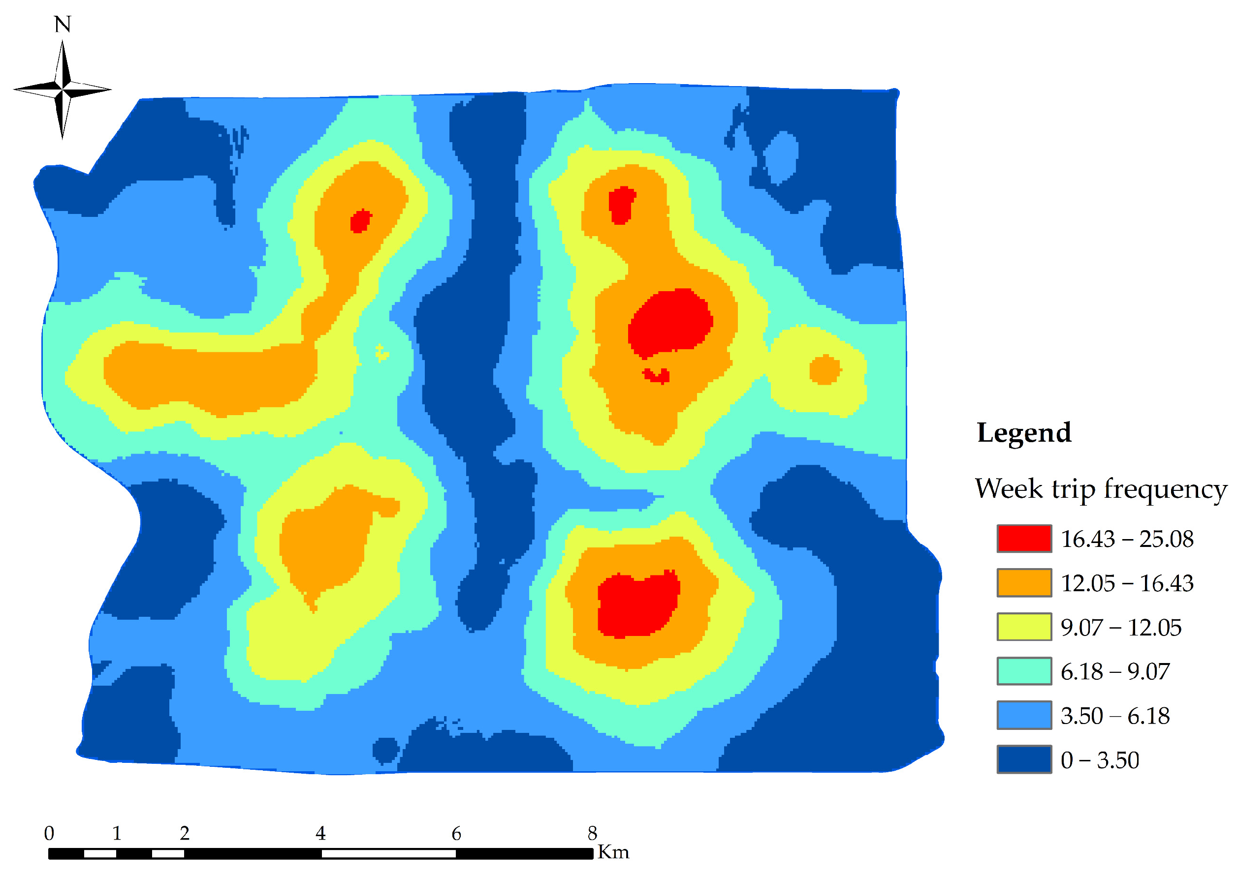
The spatial distribution of the older adults’ walking activities is depicted in Figure 2. The average weekly trip frequency of older adults is 9.01. It can be seen from the figure that their weekly trip frequency shows an obvious “circle-layer” structure in the Wanbailin district, Xinghualing district, Yingze district, and Xiaodian district, which is specifically manifested as higher in the center and lower in the periphery. The Fenhe River divides the overall weekday walking trip frequency of the older adults into two regions. In the eastern part, the higher value of the weekly trip frequency is between 16.43~25.08. However, there is a downward trend in the western region (most of the higher value ranges are 12.05~16.43), indicating that the weekly trip frequency is closely related to the population density (see Figure 1).
The personal information of the older adults is shown in Table 2. Older women and those with rural household registration are overrepresented at 51.80% and 52.38%, respectively. The percentage of retired older adults is greater, reaching 55.97%. The household income of most of the older adults is between RMB 20,000 and 80,000 (68.37%), and 23.75% of the older adults have physical disabilities.
Table 3 contains the statistical data for the variables of the neighborhood built environment. The mean residential density is 11.13/1000 m2 and the mean land use mixture is 0.72, indicating that most elderly citizens reside in densely populated neighborhoods and that the diversity of land use is generic. There are nine road intersections, twenty sidewalks, and four bus stops per buffer zone, indicating that travel is relatively convenient in the survey area. From a retail establishment, restaurant, recreation, and public service perspective, the mean number of recreation facilities in the neighborhood is relatively low, indicating that the entertainment facilities in the survey area may not be able to accommodate the diversified leisure-related travel of older adults.

3.2. Model Method

3.2.1. MGWR Model

The introduction of GWR serves as the theoretical foundation for MGWR. Based on the non-parametric methods of locally weighted regression, GWR embeds the data of the geographic location into the regression parameters to enable a point-by-point estimation and obtain the spatial effect [53], as follows:
Y i = β 0 ( u i , v i ) + k = 1 m β k ( u i , v i ) X i k + ε i , i = 1 , 2 , , n
where ( u i , v i ) denotes the residential location coordinates of the i th older adult, Y i represents the weekly walking trip frequency of the i th older adult, X i k denotes the k th neighborhood built environment variable of the i th older adult, β 0 ( u i , v i ) represents the intercept of the model, β k ( u i , v i ) denotes the regression coefficient of the k th neighborhood built environment variable and the weekly walking trip frequency of the i th older adult, ε i is the error term of the i th older adult, n represents the number of samples (older adults), and m is the number of neighborhood built environment variables.
However, GWR cannot account for the varying spatial scales of variables within the built environment of a neighborhood. Therefore, Fotheringham et al. [40] proposed the MGWR, which permits each built environment variable within a neighborhood to have its own spatial scale. The formula is as follows:
Y i = β 0 ( u i , v i ) + k = 1 m β b k ( u i , v i ) X i k + ε i , i = 1 , 2 , , n
where b k represents the bandwidth used for the regression coefficient of the k th neighborhood built environment variable (or the number of adjacent sample points in a function projection), and β b k ( u i , v i ) is similar to β k ( u i , v i ) and is considered in MGWR.
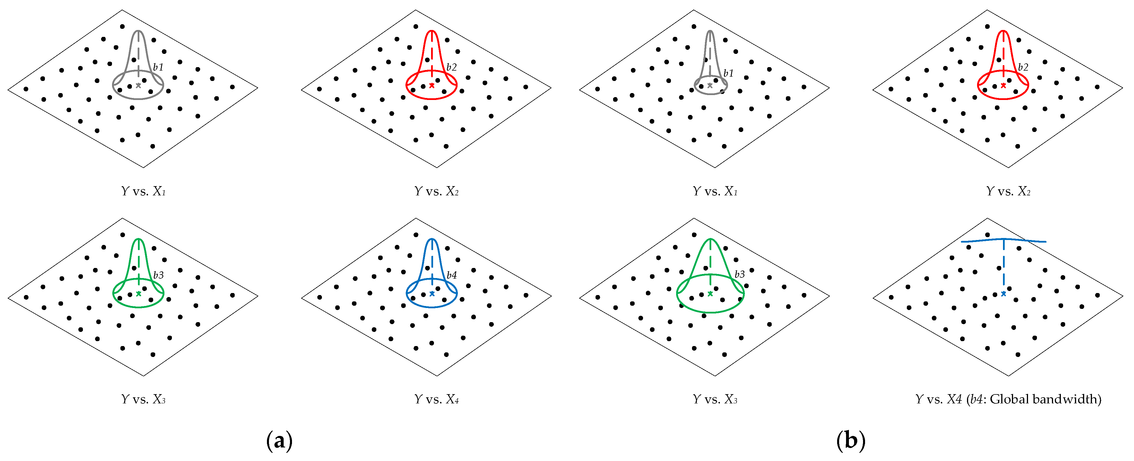
Compared to GWR, the primary advantage of MGWR is the consideration of the spatial heterogeneity between the neighborhood built environment variables [40,41,42,43]. As shown in Figure 3, GWR mandates that the bandwidth of the neighborhood built environment variables be identical and equal to the mean value. However, MGWR recognizes that the bandwidths of neighborhood built environment variables can vary, indicating that each neighborhood built environment variable has its own appropriate bandwidth.

3.2.2. Model Weight

As with GWR, the spatial weight of MGWR is described using the Gaussian kernel function, as follows:
W i = [ w i 1 0 0 0 0 0 w i 2 0 0 0 0 0 w i j 0 0 0 0 0 w i n ]
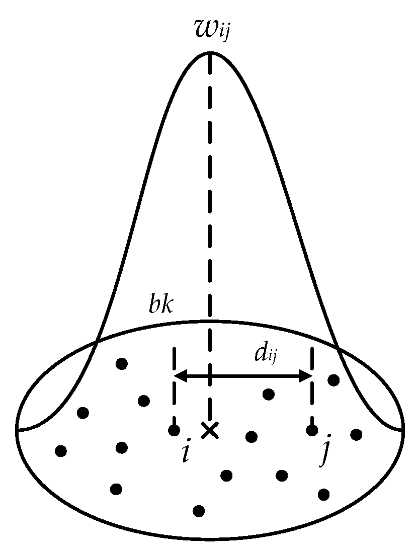
w i j = e 1 2 ( d i j b k ) 2
where W i represents the spatial weight matrix of the i th older adult, w i j denotes the spatial weight of the j th old adult in relation to the i th old adult, d i j is the distance between the i th and the j th older adult, and b k is the number of adjacent sample points in the Gaussian kernel function projection for the i th old adult.
The Gaussian kernel function of the spatial weight matrix element w i j is shown as follows (Figure 4):
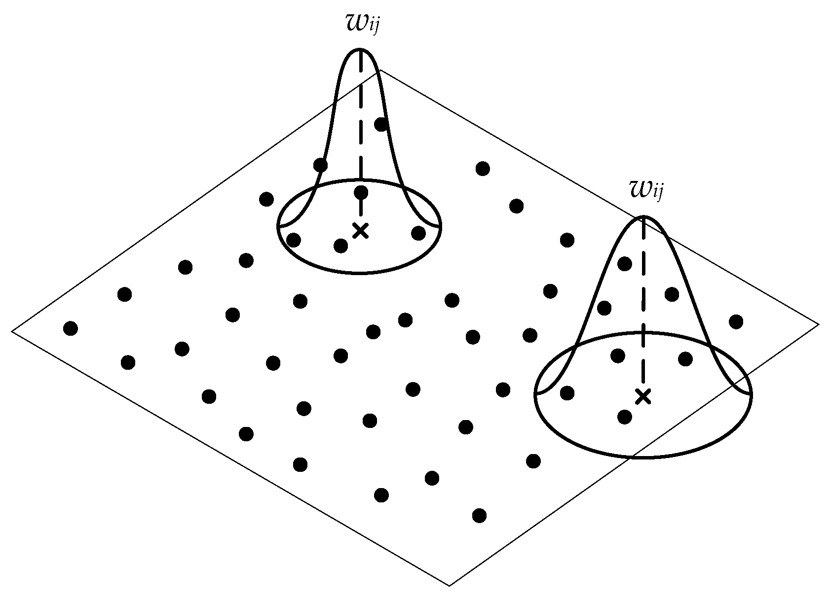
This study determines the bandwidth b k through two steps. In the first step, the Gaussian kernel function is projected onto the geographical space using the adaptive kernel by considering the adjacent sample points, as the adaptive method is more capable of dealing with the uneven spatial distribution and irregular regional periphery [41]. The second step involves determining the bandwidth using the golden section method and the corrected Akaike information criterion (AICc), as shown in Figure 5.

3.2.3. Model Estimation

The regression coefficient in MGWR is estimated based on the calculation of GWR using OLS, which can be considered a generalized additive model [54] and is presented in Equation (6):
Y = k = 1 m f k + ε
f k = β b k X k
where f k represents the k th additive item, ε denotes the residual term of the model, and X k represents the k th neighborhood built environment variable.
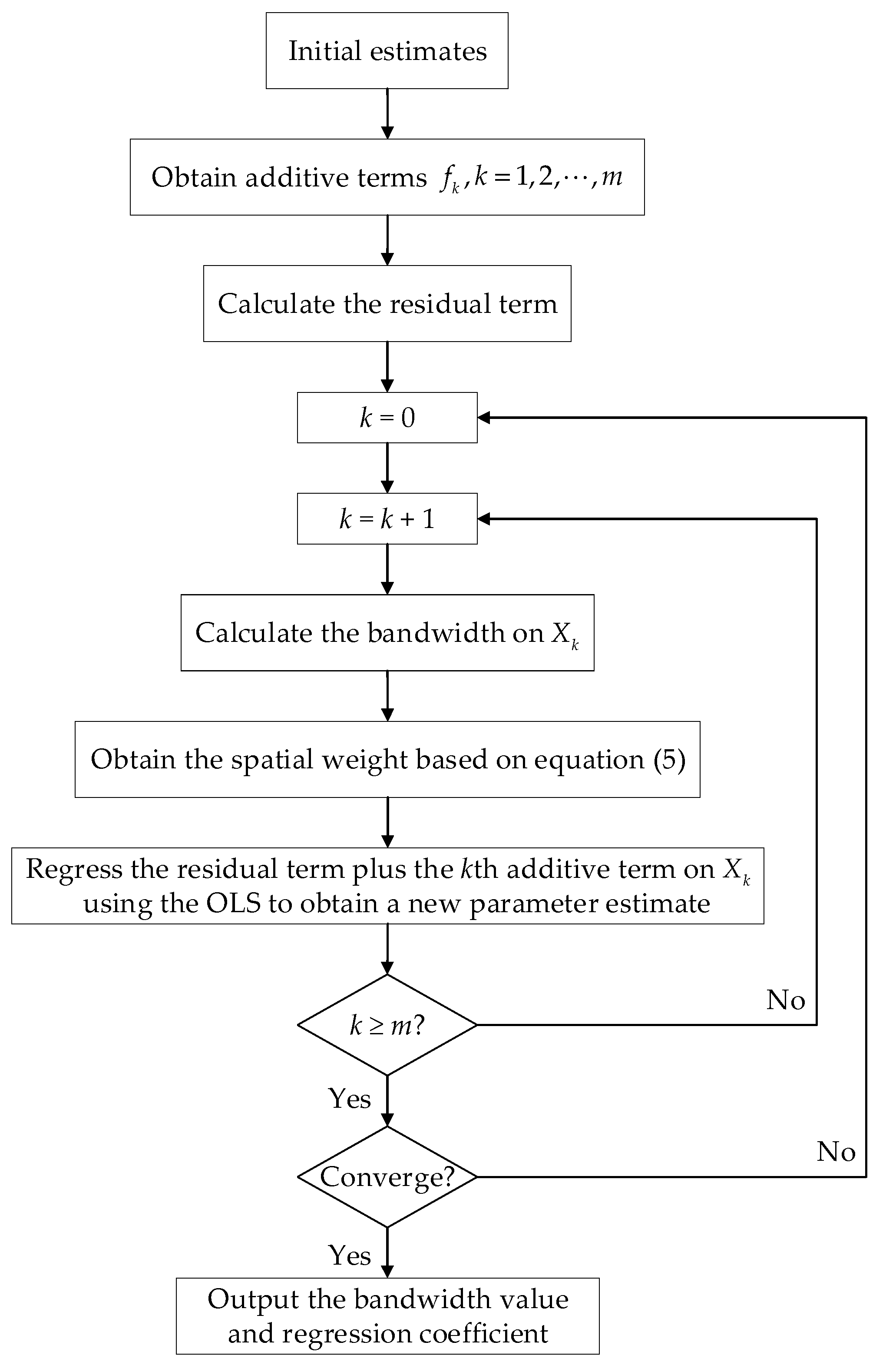
The parameter estimation of the generalized additive model can be calculated by calibrating each item using the back-fitting algorithm based on the smoothing method [40,41,42]. A flow chart of the back-fitting algorithm is shown in Figure 6, including the following steps:
Step 1: The evaluation results of GWR are selected as the initial estimates.
Step 2: Obtain the additive terms f k from the initial estimates.
Step 3: Calculate the difference between the actual and predicted values, i.e., the residual term of the model ε .
Step 4: The bandwidth b k is calculated (see the end of the model method, Section 3.2).
Step 5: The spatial weight is obtained based on Equation (5).
Step 6: The residual term plus the k th additive term ε + f k is regressed on X k to obtain a new parameter estimate using the OLS.
Step 7: If k m , proceed to the next step; otherwise, return to step 4.
Step 8: If SOC R S S reaches a minimum value in the iteration, proceed to the next step; otherwise, return to step 4. The formula for SOC R S S is as follows:
SOC R S S = | RSS n e w RSS old RSS n e w |
where RSS old denotes the residual sum of the squares in the previous step, and RSS n e w represents the residual sum of the squares in this step.
Step 9: Yield the bandwidth value and final regression coefficient of each neighborhood built environment variable.

3.2.4. Model Evaluation

In this study, we also use four common indices to compare the evaluation results of OLS, GWR, and MGWR, including the R 2 , adjusted R 2 , AICc value, and residual sum of squares. Among these indices, R 2 is a classic index used to measure the goodness-of-fit of the model. If R 2 is closer to 1, it indicates that the fitting effect is better [55]. The formula for R 2 is as follows:
R 2 = 1 ( Y i Y ^ i ) 2 ( Y i Y ¯ ) 2
where Y ^ i represents the fitting value of the weekly walking trip frequency of the i th older adult, and Y ¯ is the average value of the weekly walking trip frequency of all the older adults.
However, R 2 is usually replaced by the adjusted R 2 in the practical analysis. The adjusted R 2 is the index that eliminates the influence of the variable number on R 2 [55]. The formula for the adjusted R 2 is expressed as:
A d j . R 2 = 1 [ ( 1 R 2 ) ( n 1 ) ( n m 1 ) ]
Furthermore, the evaluation criteria of the AICc value and residual sum of squares are the same. If the value is smaller, then the model fitting effect is better [43,55].

4. Results

4.1. Variable Inspection

Figure 7 shows the spatial autocorrelation of the weekly walking trip frequency of the older adults based on the global Moran’s I theory. In the study area, the Moran’s index is 0.65, the z-score is 10.93, and the p-value is 0.00, indicating that older adults’ weekly walking trip frequency has a significant spatial clustering effect (the weekly walking trip frequency of 297 older adults has a high–high cluster distribution, and that of 270 older adults has a low–low cluster distribution). This indicates that the MGWR is more appropriate for studying changes in the spatial location and that the weekly walking trip frequency of older adults can accurately represent their walking activities.
Then, the tolerance and variance inflation factor (VIF) are employed to select statistically significant variables via collinearity diagnosis [6,20]. As shown in Table 4, it is found that the number of road intersections and the number of pedestrian crossings have a collinearity problem in the first collinearity diagnosis. In the final collinearity diagnosis, the number of road intersections is eliminated because there is no collinearity problem among explanatory variables. Therefore, the explanatory variables from the final diagnosis of collinearity are utilized in the subsequent analysis.

4.2. Model Comparison

Table 5 compares the model evaluation results of OLS, GWR, and MGWR to demonstrate the superiority of MGWR in analyzing the effect of the neighborhood built environment on the walking activities of older adults. In terms of the R 2 , adjusted R 2 , AICc value, and residual sum of squares, GWR and MGWR are better than OLS, indicating that OLS omits the spatial changes in the samples [6,43]. Comparing GWR and MGWR, they show little difference in the R 2 , adjusted R 2 , and residual sum of squares. However, in terms of the AICc value, MGWR is superior to GWR, which indicates that GWR ignores the scale differences between the explanatory variables [43].
The bandwidth of OLS is non-existent because it considers the global spatial distribution rather than the local spatial distribution. Hence, the research team further compared the bandwidth differences between GWR and MGWR. Table 6 demonstrates that MGWR can directly reflect the varying scales of various explanatory variables, whereas GWR can only obtain the average scale of all the explanatory variables [40,41,42], i.e., GWR has a bandwidth of 71. In the MGWR, the bandwidth of the location, land use mixture, the number of pedestrian crossings, the number of retail establishments, and the number of restaurants is 43, representing 4.98% of the sample size, while the bandwidths of the residential density and number of bus stops are 46 and 48, representing 5.33% and 5.56% of the sample size, respectively. Consequently, these explanatory variables exhibit spatial heterogeneity. However, the bandwidth of the number of recreation facilities and the number of public service facilities is 862, which indicates that these two explanatory variables are relatively stable in terms of geographic space. These results indicate that MGWR can produce regression results that are more representative of the actual value and actual situation than GWR.

4.3. Spatial Feature

The parameter estimation generated by MGWR can reflect the spatial heterogeneity resulting from the built environment’s effect on the walking activities of older adults [42]. The statistical description of the regression coefficients is shown in Table 7. Note that the location is equivalent to the model’s intercept, which is a new explanatory variable. According to the mean value of the regression coefficient, the variables excluding the location are related to the increase in the older adults’ weekly frequency of walking trips. The minimum and maximum values of the regression coefficient indicate that other explanatory variables have both positive and negative effects on the weekly walking trip frequency of older adults, in addition to the number of recreation facilities and the number of public service facilities.
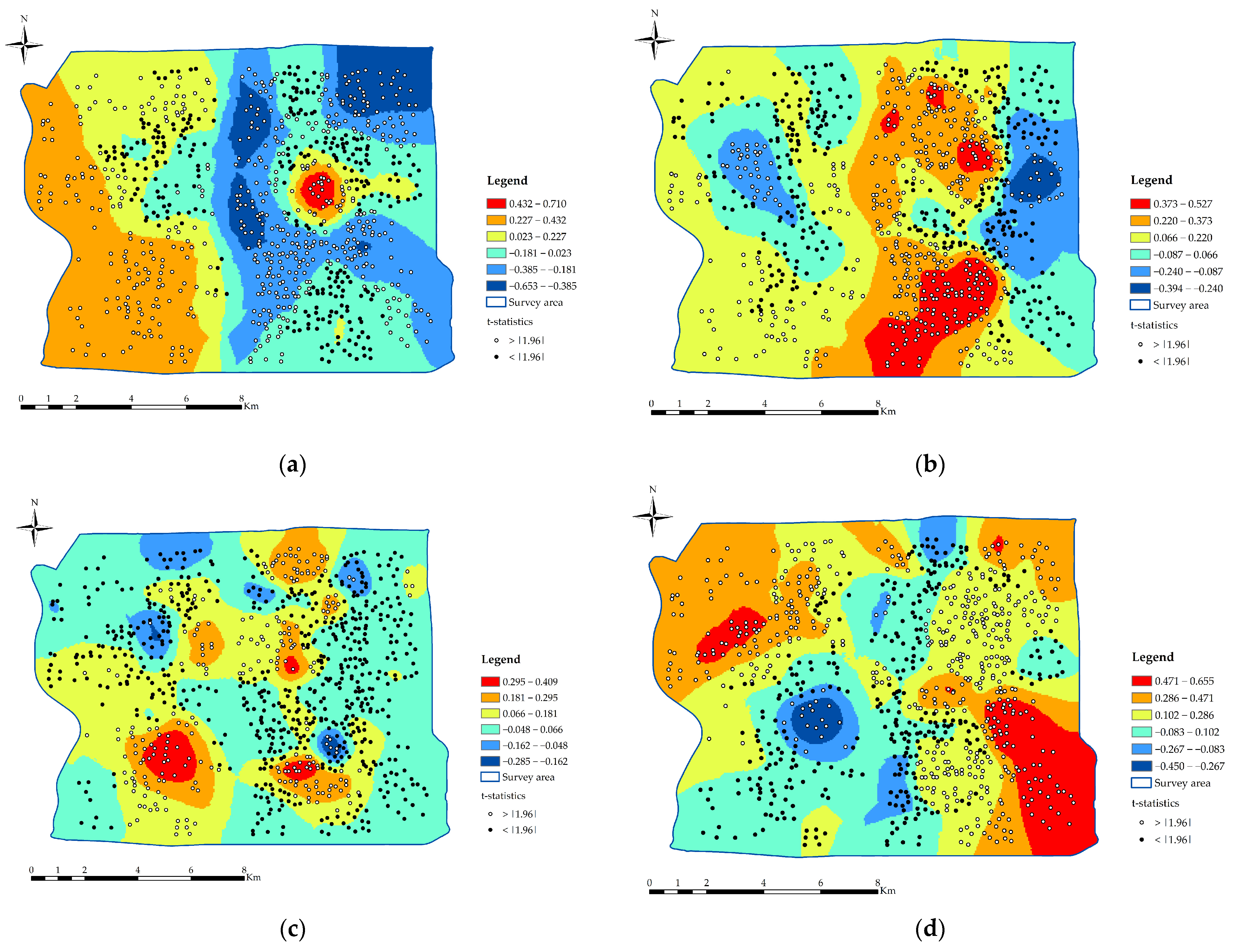
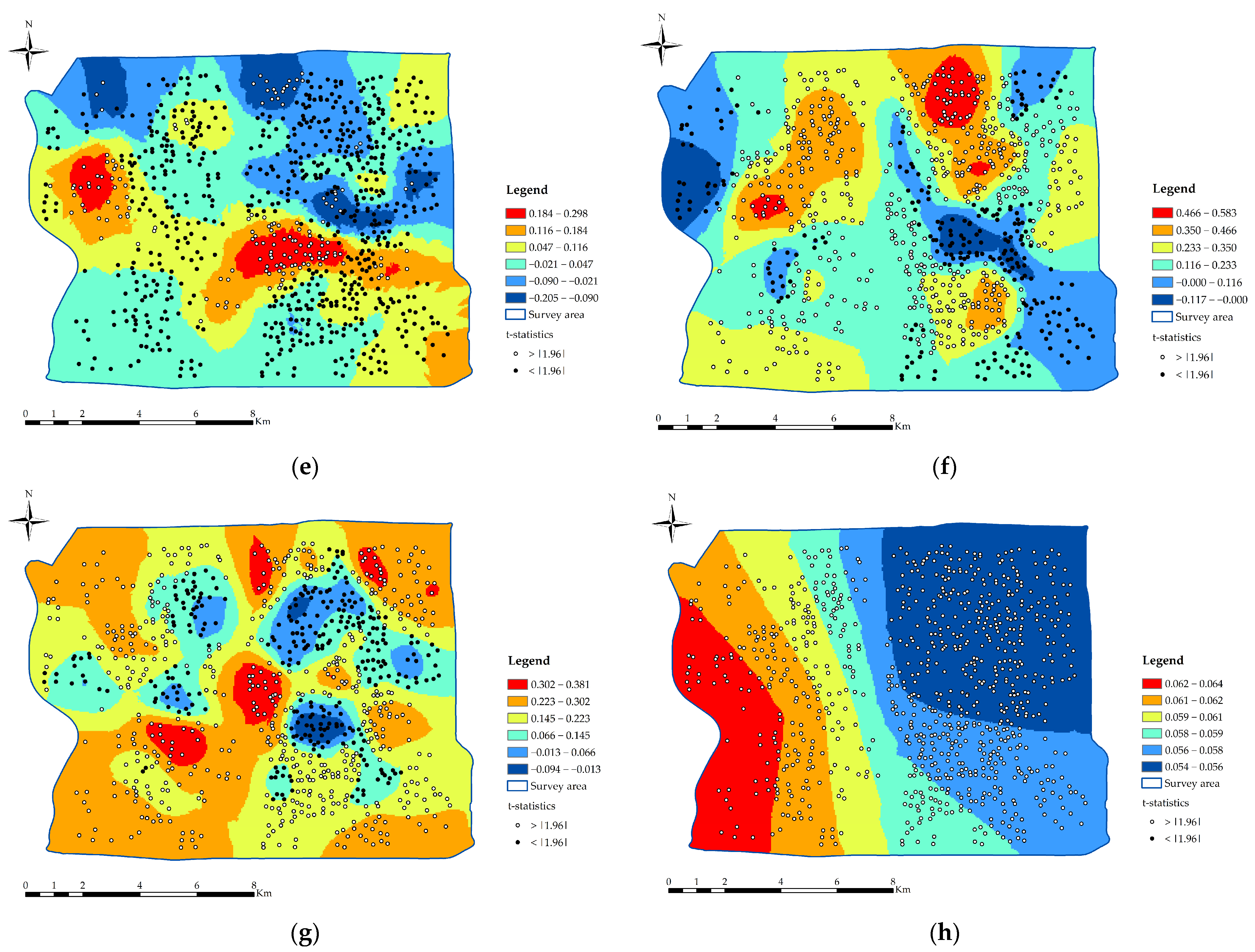
Figure 8 depicts a geospatial visualization of the study area that can be used to analyze the influence of each explanatory variable on the walking of older adults, with t-statistics used to demonstrate the significant effects of the residential location on older adults’ activities. There is a certain correlation between the entire study area and the neighborhood, as the influence effect in the study area is based on 863 neighbors (one older adult is counted as a neighborhood). Additionally, the influence effects of two neighbors under the same explanatory variable are similar in the study area. All regression coefficients and t-statistics are shown in Table S2 of Supplementary Materials. The number of public service facilities is not discussed in the following analysis because its regression coefficient is not statistically significant.
  • Location
The location regression coefficient ranges from −0.653 to 0.710, with a mean value of −0.056 and SD of 0.257. The areas with significant effects are the southwestern part of the Wanbailin district, Xinghualing district, Yingze district, and the northern part of Xiaodian district, as shown in Figure 8a. Based on the absolute value of the coefficient, its influence intensity is generic among all the explanatory variables. The spatial differences in location between different regions are larger. Higher values are primarily concentrated in the central part of the Yingze district, whereas lower values are primarily concentrated in the northern part of the Xinghualing district and the east side of the Fenhe River. This indicates that a neighborhood with a good location can encourage older adults to walk to some extent, but not vice versa. For instance, in the central part of the Yingze district, the weekly trip frequency of older adults who walk can increase by 0.432~0.710 when the location increases by one unit. However, in the northeastern part of the Xinghualing district, the weekly walking trip frequency among older adults can decrease by 0.385~0.653 when the location increases by one unit.
  • Residential density
The residential density regression coefficient ranges between −0.394 and 0.527, with a mean value of 0.142 and SD of 0.186. The areas with significant effects are the southern part of the study area and the Xinghualing district, as shown in Figure 8b. In terms of the coefficient’s absolute value, its influence intensity is greater, as are the spatial differences between regions. Higher values are concentrated in the districts of Xiaodian and Xinghualing, while lower values are concentrated in the northern part of the Wanbailin district and the eastern part of the study area. This means that older adults living in high-density neighborhoods often travel together, which promotes their activities, such as walking and socializing, and reduces the instance of sedentary lifestyles. This finding is similar to that of Chaudhury et al. [56], who reported that older adults living in high-density neighborhoods are more likely to form groups. Moreover, the transportation facilities in high-density residential environments are more comprehensive than those in low-density residential environments, which may also improve older adults’ walking quality.
  • Land use mixture
The regression coefficient of the land use mixture is between −0.285 and 0.409, with a mean value of 0.078 and SD of 0.106. As shown in Figure 8c, the areas with significant effects are the southern part of the Wanbailin district, the western part of the Xinghualing district, and the Xiaodian district. The absolute value of the coefficient indicates that the intensity of the influence is generic, indicating that the spatial variation in the land use mixture in various regions is also generic. Higher values are concentrated in the southern part of the Wanbailin district, while lower values are concentrated within the local scope of the study area as a whole. The results indicate that a greater variety of land use types can provide more opportunities for walking activities among older adults [6,30]. For instance, in the southern part of the Wanbailin district, the weekly trip frequency of older adults who walk can increase by 0.295~0.409 if the land use mixture increases by one unit. Nonetheless, older adults in high-mixed neighborhoods may undertake multiple trips for a travel purpose, thereby reducing their walking trip frequency, as in the northern part of the Xiaodian district [6].
  • Number of pedestrian crossings
The regression coefficient for the number of pedestrian crossings ranges from −0.450 to 0.655, with a mean value of 0.191 and SD of 0.190. The areas with significant effects are the northwestern and eastern parts of the study area, as shown in Figure 8d. Regarding the regression coefficient, its intensity of influence is greater, as is the difference in influence between regions. Higher values are mainly concentrated in the study area’s perimeter, while lower values are mainly concentrated in the study area’s interior. This difference can be explained by the fact that in the interior of the study area (e.g., the central part of the Wanbailin district), the pedestrian crossings are often crowded and noisy and more likely to be damaged and occupied than those in the periphery due to the higher population density, which affects the walking activities of older adults.
  • Number of bus stops
The regression coefficient for the number of bus stops ranges from −0.205 to 0.298, with a mean of 0.035 and SD of 0.092. The areas with significant effects are the western part of the Wanbailin district, the northern part of the Xiaodian district, and the Jiancaoping district, as shown in Figure 8e. Regarding the absolute value of the coefficient, the intensity of its influence is lower, indicating that the spatial difference in the number of bus stops between regions is common. The higher values are concentrated in the western part of the Wanbailin district and the northern part of the Xiaodian district, and the lower values are concentrated in the Jiancaoping district and Yingze district. This indicates that providing more neighborhoods with bus stops may contribute to the walking activities of older adults [30,57] because bus trips are always accompanied by walking to and from bus stops and walking constitutes a portion of each trip [6,58]. For example, in the northern part of the Xiaodian district, the weekly walking trip frequency among older adults can increase by 0.184~0.298 when the number of bus stops increases by one unit.
  • Number of retail establishments
The regression coefficient of the number of retail establishments is between −0.117 and 0.583, with a mean value of 0.235 and SD of 0.146. The areas with significant effects are the northern part of the Wanbailin district, Xinghualing district, Yingze district, and Xiaodian district, as shown in Figure 8f. This variable has the greatest impact on the analysis of the regression coefficients, and the spatial differences between regions are also the greatest. The higher values are concentrated in the Xinghualing district and the northern part of the Yingze district. Lower values are concentrated in the western part of the Wanbailin and the southern part of Yingze. This indicates that retail establishments (such as stores and markets) are more accessible and convergent, thereby meeting the needs of older adults to some extent [57]. Furthermore, if the number of retail establishments is excessive in well-developed economic areas with high population densities, the crowding phenomenon of walking activities occurs frequently [58], resulting in a decline in outdoor activities among older adults, as in the Xiaodian district.
  • Number of restaurants
The regression coefficient for the number of restaurants ranges from −0.094 to 0.381, with a mean of 0.172 and SD of 0.091. The areas with significant effects are the local area of the Wanbailin district, Xiaodian district, and the northeastern part of the study area, as shown in Figure 8g. In terms of the absolute value of the coefficient, its influence intensity is greater, and regional spatial disparities are prevalent. Higher values are concentrated in the northeastern part of the Xinghualing district and the western part of the Yingze district, and the lower values are concentrated in the western and central parts of the Xinghualing district and the northern part of the Xiaodian district. This demonstrates that there are many restaurants and food courts in close proximity to the neighborhood, which increases the likelihood that older adults will eat out, thereby increasing their walking trips [32], as in the northeastern part of the Xinghualing district. Nonetheless, based on Figure 2 and Figure 8g, we found that the number of restaurants has a negative effect on the walking activities of older adults. The reason for this is that most restaurants mainly cater to the tastes of young people and lack basic, barrier-free indoor facilities for older adults.
  • Number of recreation facilities
The number of recreation facilities has a regression coefficient between 0.054 and 0.064, with a mean value of 0.057 and SD of 0.003. As shown in Figure 8h, the areas with significant effects are the entire study area. Regarding the regression coefficient, its influence degree is generic. Nonetheless, the spatial differences between regions are smaller, exhibiting a “step-like” structure from west to east. The higher values are concentrated in the Wanbailin district, and the lower values are concentrated in the Xinghualing district and Yingze district. This indicates that the number of recreational facilities affects the total walking activities of older adults. In Section 3.1, on data sources, we found that the number of recreation facilities in each buffer zone is low (the mean value is 1.22). These results further support the conclusion, i.e., the fact that “the entertainment facilities in the survey area may not be able to meet the diversified leisure travel of older adults”, mentioned at the end of Section 3.1.

5. Conclusions

Using Taiyuan as a case study, in this paper, we employed MGWR to examine the effect of the built environment on older adults’ walking activities. This study demonstrates that the built environment of a neighborhood is strongly associated with the walking activities of older adults, and that these relationships vary geographically.
The main results are presented below.
Previous studies based on OLS and GWR have flaws, whereas MGWR can reflect the spatial scales of various explanatory variables, resulting in more reliable regression results. The spatial scales of the location, residential density, land use mixture, number of pedestrian crossings, number of bus stops, number of retail establishments, and number of restaurants are smaller, whereas the spatial scales of the number of recreation facilities and number of public service facilities are global across the study area.
Regarding the walking activities of older adults, the pattern of the influence intensity, moving from higher to lower, is the number of retail establishments, number of pedestrian crossings, number of restaurants, residential density, land use mixture, the number of recreation facilities, location, and the number of bus stops. The location, residential density, the number of pedestrian crossings, and the number of retail establishments are the major spatial differences. The generic spatial differences are the mixture of land use types, the number of bus stops, and the number of restaurants, while the effect of the number of recreation facilities in each neighborhood is small, and its spatial difference is minimal.
In light of our findings, the following six policies are proposed:
(a) Some attractive places for older adults (such as activity centers) should be added to neighborhoods in poor locations, such as the northeastern part of the study area.
(b) Pedestrian crossings should be checked frequently and crossing facilities (such as underground passages and overpasses) should be increased in neighborhoods with a high population density, e.g., in the eastern part of the study area.
(c) The planning of bus stops in each neighborhood should be improved, and in the northern part of the study area, attention should be paid to the effective connection between the residential locations of older adults and attractive places (such as retail establishments, restaurants, and recreation).
(d) The arrangement of retail establishments should consider the connection with neighborhoods. However, this must be implemented with caution, because a high number of these establishments may increase street congestion, thereby affecting the walking activities of older adults.
(e) Restaurants for senior citizens should be expanded and placed in convenient areas, particularly in the western and central parts of the Xinghualing and Xiaodian districts.
(f) Recreational facilities for older adults should be planned and built to enhance the recreational trips and quality of life of older adults in all street spaces and building structures within the study area.
These findings can not only aid researchers and urban planners in comprehending the relationship between the built environment of a neighborhood and the walking activities of older adults but also contribute to the sustainable development of a “walking-friendly” transportation city system for older adults. Nonetheless, this study has limitations that must be addressed in future research. At the data source level, additional explanatory variables should be added, such as the street connectivity [6] and perceptions of the built environment [59]. At the model method level, the temporal dimension should be introduced to enrich the research on the walking activities of older adults. At the result analysis level, more quantitative studies (e.g., quasi-experimental analysis) are required [6,60]. In addition, the proposed MGWR should be applied to analyses of the travel behavior of other populations to demonstrate its reliability and applicability.

Supplementary Materials

The following supporting information can be downloaded at: https://www.mdpi.com/article/10.3390/su142113927/s1, Table S1 is the data of week trip frequency for walking of older adults, related to the residential density, land use mixture, number of road in-tersections, number of pedestrian crossings, number of bus stops, number of retail establishments, number of restaurants, number of recreation facilities, and number of public-service facilities (Section 3.1); Table S2 shows the output results of MGWR, including regression coefficients and t-statistics (Section 4.3).

Author Contributions

In this paper, Q.J. and T.Z. conceived the idea and wrote the article. L.C., G.C., and M.J. provided guidance, comments, and key suggestions. This version was read and approved by all the authors. All authors have read and agreed to the published version of the manuscript.

Funding

This work was supported in part by the National Natural Science Foundation of China (grant No. 51968063), in part by the Fundamental Research Program of Shanxi Province (grant Nos. 20210302124455 and 202103021223301), in part by the research project supported by the Shanxi Scholarship Council of China (grant No. 2022-159), in part by the Excellent Doctor Award Fund for Work in Shanxi (grant Nos. 20202029 and 20212057), and in part by the Scientific and Technological Innovation Programs of Higher Education Institutions in Shanxi (grant Nos. 2020L0348 and 2021L335).

Institutional Review Board Statement

Not applicable.

Informed Consent Statement

Not applicable.

Data Availability Statement

Data are contained within the article. Any elaborations are available, upon request, from the authors.

Acknowledgments

The authors would like to thank the editor, Natrika Sirinapaspokin, and anonymous referees for their valuable comments and suggestions on the earlier drafts of the paper. We are also grateful to the investigators and respondents, who helped with our data collection.

Conflicts of Interest

The authors declare no conflict of interest.

References

  1. World Health Organization. Caring for the Health of the Elderly in China; World Health Organization: Geneva, Switzerland, 2021.
  2. Barnett, D.W.; Barnett, A.; Nathan, A.; Van Cauwenberg, J.; Cerin, E. Built environmental correlates of older adults’ total physical activity and walking: A systematic review and meta-analysis. Int. J. Behav. Nutr. Phys. Act. 2017, 14, 103. [Google Scholar] [CrossRef] [PubMed] [Green Version]
  3. Cerin, E.; Nathan, A.; Van Cauwenberg, J.; Barnett, D.W.; Barnett, A. The neighbourhood physical environment and active travel in older adults: A systematic review and meta-analysis. Int. J. Behav. Nutr. Phys. Act. 2017, 14, 15. [Google Scholar] [CrossRef] [PubMed] [Green Version]
  4. Amaya, V.; Chardon, M.; Klein, H.; Moulaert, T.; Vuillerme, N. What do we know about the use of the walk-along method to identify the perceived neighborhood environment correlates of walking activity in healthy older adults: Methodological considerations related to data collection—A systematic review. Sustainability 2022, 14, 11792. [Google Scholar] [CrossRef]
  5. Feuillet, T.; Commenges, H.; Menai, M.; Salze, P.; Perchoux, C.; Reuillon, R.; Kesse-Guyot, E.; Enaux, C.; Nazare, J.A.; Hercberg, S.; et al. A massive geographically weighted regression model of walking-environment relationships. J. Transp. Geogr. 2018, 68, 118–129. [Google Scholar] [CrossRef]
  6. Cheng, L.; Shi, K.; De Vos, J.; Cao, M.; Witlox, F. Examining the spatially heterogeneous effects of the built environment on walking among older adults. Transp. Policy 2021, 100, 21–30. [Google Scholar] [CrossRef]
  7. Yun, H.Y. Neighborhood built environments, walking, and self-rated health among low-income older adults in St. Paul, Minnesota. Sustainability 2021, 13, 3501. [Google Scholar] [CrossRef]
  8. Herbolsheimer, F.; Mahmood, A.; Ungar, N.; Michael, Y.L.; Oswald, F.; Chaudhury, H. Perceptions of the neighborhood built environment for walking behavior in older adults living in close proximity. J. Appl. Gerontol. 2021, 40, 1697–1705. [Google Scholar] [CrossRef]
  9. Kemperman, A.; Timmermans, H. Influences of built environment on walking and cycling by latent segments of aging population. Transport. Res. Rec. 2009, 2134, 1–9. [Google Scholar] [CrossRef]
  10. Gong, Y.; Gallacher, J.; Palmer, S.; Fone, D. Neighbourhood green space, physical function and participation in physical activities among elderly men: The Caerphilly Prospective study. Int. J. Behav. Nutr. Phys. Act. 2014, 11, 40. [Google Scholar] [CrossRef] [Green Version]
  11. Gómez, L.F.; Parra, D.C.; Buchner, D.; Brownson, R.C.; Sarmiento, O.L.; Pinzón, J.D.; Moreno, J.; Lobelo, F. Built environment attributes and walking patterns among the elderly population in Bogotá. Am. J. Prev. Med. 2010, 38, 592–599. [Google Scholar] [CrossRef]
  12. Cheng, L.; De Vos, J.; Shi, K.; Yang, M.; Chen, X.; Witlox, F. Do residential location effects on travel behavior differ between the elderly and younger adults? Transp. Res. D Transp. Environ. 2019, 73, 367–380. [Google Scholar] [CrossRef]
  13. Zhang, Y.; Li, C.; Ding, C.; Zhao, C.; Huang, J. The built environment and the frequency of cycling trips by urban elderly: Insights from Zhongshan, China. J. Asian Archit. Build. 2016, 15, 511–518. [Google Scholar] [CrossRef]
  14. Paydar, M.; Fard, A.K.; Khaghani, M.M. Walking toward metro stations: The contribution of distance, attitudes, and perceived built environment. Sustainability 2020, 12, 10291. [Google Scholar] [CrossRef]
  15. Cerin, E.; Sit, C.H.P.; Barnett, A.; Johnston, J.M.; Cheung, M.C.; Chan, W.M. Ageing in an ultra-dense metropolis: Perceived neighbourhood characteristics and utilitarian walking in Hong Kong elders. Public Health Nutr. 2012, 17, 225–232. [Google Scholar] [CrossRef] [PubMed]
  16. Feuillet, T.; Salze, P.; Charreire, H.; Menai, M.; Enaux, C.; Perchoux, C.; Hess, F.; Kesse-Guyot, E.; Hercberg, S.; Simon, C.; et al. Built environment in local relation with walking: Why here and not there? J. Transp. Health 2016, 3, 500–512. [Google Scholar] [CrossRef]
  17. Böcker, L.; Van Amen, P.; Helbich, M. Elderly travel frequencies and transport mode choices in Greater Rotterdam, the Netherlands. Transportation 2016, 44, 831–852. [Google Scholar] [CrossRef] [Green Version]
  18. Lee, E.; Dean, J. Perceptions of walkability and determinants of walking behaviour among urban seniors in Toronto, Canada. J. Transp. Health 2018, 9, 309–320. [Google Scholar] [CrossRef]
  19. Ding, C.; Lin, Y.; Liu, C. Exploring the influence of built environment on tour-based commuter mode choice: A cross-classified multilevel modeling approach. Transp. Res. D Transp. Environ. 2014, 32, 230–238. [Google Scholar] [CrossRef]
  20. Ma, X.; Zhang, J.; Ding, C.; Wang, Y. A geographically and temporally weighted regression model to explore the spatiotemporal influence of built environment on transit ridership. Comput. Environ. Urban 2018, 70, 113–124. [Google Scholar] [CrossRef]
  21. Cheng, L.; Wang, K.; De Vos, J.; Huang, J.; Witlox, F. Exploring non-linear built environment effects on the integration of free-floating bike-share and urban rail transport: A quantile regression approach. Transp. Res. Part A Policy Pract. 2022, 162, 175–187. [Google Scholar] [CrossRef]
  22. Hanibuchi, T.; Kawachi, I.; Nakaya, T.; Hirai, H.; Kondo, K. Neighborhood built environment and physical activity of Japanese older adults: Results from the Aichi Gerontological Evaluation Study (AGES). BMC Public Health 2011, 11, 657. [Google Scholar] [CrossRef] [PubMed] [Green Version]
  23. Xiao, L.; Yang, L.; Liu, J.; Yang, H. Built environment correlates of the propensity of walking and cycling. Sustainability 2020, 12, 8752. [Google Scholar] [CrossRef]
  24. Ewing, R.; Cervero, R. Travel and the built environment: A meta-analysis. J. Am. Plan. Assoc. 2010, 76, 265–294. [Google Scholar] [CrossRef]
  25. Smith, G.; Gidlow, C.; Davey, R.; Foster, C. What is my walking neighbourhood? A pilot study of English adults’ definitions of their local walking neighbourhoods. Int. J. Behav. Nutr. Phys. Act. 2010, 7, 34. [Google Scholar] [CrossRef] [PubMed] [Green Version]
  26. Ding, C.; Cao, X.; Wang, Y. Synergistic effects of the built environment and commuting programs on commute mode choice. Transp. Res. A Policy Pract. 2018, 118, 104–118. [Google Scholar] [CrossRef]
  27. Yang, H.; Zhai, G.; Yang, L.; Xie, K. How does the suspension of ride-sourcing affect the transportation system and environment? Transp. Res. D Transp. Environ. 2022, 102, 103131. [Google Scholar] [CrossRef]
  28. Nagel, C.L.; Carlson, N.E.; Bosworth, M.; Michael, Y.L. The relation between neighborhood built environment and walking activity among older adults. Am. J. Epidemiol. 2008, 168, 461–468. [Google Scholar] [CrossRef] [Green Version]
  29. Zhang, Y.; Li, Y.; Liu, Q.; Li, C. The built environment and walking activity of the elderly: An empirical analysis in the Zhongshan metropolitan area, China. Sustainability 2014, 6, 1076–1092. [Google Scholar] [CrossRef] [Green Version]
  30. Feng, J. The influence of built environment on travel behavior of the elderly in urban China. Transp. Res. D Transp. Environ. 2016, 52, 619–633. [Google Scholar] [CrossRef]
  31. Yang, H.; Huo, J.; Pan, R.; Xie, K.; Zhang, W.; Luo, X. Exploring built environment factors that influence the market share of ridesourcing service. Appl. Geogr. 2022, 142, 102699. [Google Scholar] [CrossRef]
  32. Hou, Y. Polycentric urban form and non-work travel in Singapore: A focus on seniors. Transp. Res. D Transp. Environ. 2019, 73, 245–275. [Google Scholar] [CrossRef]
  33. Li, Z.; Fotheringham, A.S.; Oshan, T.M.; Wolf, L.J. Measuring bandwidth uncertainty in multiscale geographically weighted regression using Akaike weights. Ann. Amer. Assoc. Geogr. 2020, 110, 1500–1520. [Google Scholar] [CrossRef]
  34. Cheng, L.; Chen, X.; Yang, S.; Cao, Z.; De Vos, J.; Witlox, F. Active travel for active ageing in China: The role of built environment. J. Transp. Geogr. 2019, 76, 142–152. [Google Scholar] [CrossRef]
  35. Cheng, L.; De Vos, J.; Zhao, P.; Yang, M.; Witlox, F. Examining non-linear built environment effects on elderly’s walking: A random forest approach. Transp. Res. D Transp. Environ. 2020, 88, 102552. [Google Scholar] [CrossRef]
  36. Engels, B.; Liu, G.J. Social exclusion, location and transport disadvantage amongst non-driving seniors in a Melbourne municipality, Australia. J. Transp. Geogr. 2011, 19, 984–996. [Google Scholar] [CrossRef]
  37. Yang, S.; Fan, Y.; Deng, W.; Cheng, L. Do built environment effects on travel behavior differ between household members? A case study of Nanjing, China. Transp. Policy 2017, 81, 360–370. [Google Scholar] [CrossRef]
  38. Hou, Y.; Moogoor, A.; Dieterich, A.; Song, S.; Yuen, B. Exploring built environment correlates of older adults’ walking travel from lifelogging images. Transp. Res. D Transp. Environ. 2021, 96, 102850. [Google Scholar] [CrossRef]
  39. Bao, J.; Shi, X.; Zhang, H. Spatial analysis of bikeshare ridership with smart card and POI data using geographically weighted regression method. IEEE Access 2018, 6, 76049–76059. [Google Scholar] [CrossRef]
  40. Fotheringham, A.S.; Yang, W.; Kang, W. Multiscale geographically weighted regression (MGWR). Ann. Am. Assoc. Geogr. 2017, 107, 1247–1265. [Google Scholar] [CrossRef]
  41. Oshan, T.M.; Li, Z.; Kang, W.; Wolf, L.J.; Fotheringham, A.S. MGWR: A python implementation of multiscale geographically weighted regression for investigating process spatial heterogeneity and scale. ISPRS Int. J. Geo-Inf. 2019, 8, 269. [Google Scholar] [CrossRef]
  42. Yu, H.; Fotheringham, A.S.; Li, Z.; Oshan, T.; Kang, W.; Wolf, L.J. Inference in multiscale geographically weighted regression. Geogr. Anal. 2020, 52, 87–106. [Google Scholar] [CrossRef]
  43. Geng, S.; Ma, M.; Hu, X.; Yu, H. Multi-scale geographically weighted regression modeling of urban and rural construction land fragmentation—A case study of the Yangtze River Delta Region. IEEE Access 2021, 10, 7639–7652. [Google Scholar] [CrossRef]
  44. Corseuil-Giehl, M.W.; Hallal, P.C.; Brownson, R.C.; d’Orsi, E. Exploring associations between perceived measures of the environment and walking among Brazilian older adults. J. Aging Health 2017, 29, 45–67. [Google Scholar] [CrossRef] [PubMed]
  45. Corseuil, M.W.; Schneider, I.J.C.; Silva, D.A.S.; Costa, F.F.; Silva, K.S.; Borges, L.J.; d’Orsi, E. Perception of environmental obstacles to commuting physical activity in Brazilian elderly. Prev. Med. 2011, 53, 289–292. [Google Scholar] [CrossRef]
  46. Gaglione, F.; Cottrill, C.; Gargiulo, C. Urban services, pedestrian networks and behaviors to measure elderly accessibility. Transp. Res. D Transp. Environ. 2021, 90, 102687. [Google Scholar] [CrossRef]
  47. Wu, H.; Wang, H.; Liu, D.; Cao, Y.; Qu, Y. The impact of the neighborhood built environment on the commuting patterns and health of patients with chronic diseases: A case study of Changshu, China. Sustainability 2022, 14, 11201. [Google Scholar] [CrossRef]
  48. Hwang, E.; Brossoie, N.; Jeong, J.W.; Song, K. The impacts of the neighborhood built environment on social capital for middle-aged and elderly Koreans. Sustainability 2021, 13, 756. [Google Scholar] [CrossRef]
  49. Gao, C.; Yu, J.; Zhao, X.; Wang, H.; Liu, Z.; Gu, Y. The effect of built environment on older people leisure-time walking and physical activity in different sex groups in the city of Ningbo, China. Sustainability 2022, 14, 6562. [Google Scholar] [CrossRef]
  50. Liu, P.; Wu, C.; Chen, M.; Ye, X.; Peng, Y.; Li, S. A spatiotemporal analysis of the effects of urbanization’s socio-economic factors on landscape patterns considering operational scales. Sustainability 2020, 12, 2543. [Google Scholar] [CrossRef] [Green Version]
  51. Yang, C.; Zhan, Q.; Lv, Y.; Liu, H. Downscaling land surface temperature using multiscale geographically weighted regression over heterogeneous landscapes in Wuhan, China. IEEE J. Sel. Topics Appl. Earth Observ. Remote Sens. 2019, 12, 5213–5222. [Google Scholar] [CrossRef]
  52. Taiyuan Bureau of Statistics. Main data bulletin of Taiyuan’s sampling survey on population change in 2021; Taiyuan Bureau of Statistics: Taiyuan, China, 2022. [Google Scholar]
  53. Fotheringham, A.S.; Brunsdon, C.; Charlton, M. Geographically Weighted Regression: The Analysis of Spatially Varying Relationships; John Wiley & Sons: Hoboken, NJ, USA, 2002. [Google Scholar]
  54. Hastie, T.; Tibshirani, R. Generalized additive models. Stat. Sci. 1986, 1, 297–318. [Google Scholar] [CrossRef]
  55. Li, Z.; Shang, Y.; Zhao, G.; Yang, M. Exploring the multiscale relationship between the built environment and the metro-oriented dockless bike-sharing usage. Int. J. Environ. Res. Public Health 2022, 19, 2323. [Google Scholar] [CrossRef] [PubMed]
  56. Chaudhury, H.; Mahmood, A.; Michael, Y.L.; Campo, M.; Hay, K. The influence of neighborhood residential density, physical and social environments on older adults’ physical activity: An exploratory study in two metropolitan areas. J. Aging Stud. 2012, 26, 35–43. [Google Scholar] [CrossRef]
  57. Herrmann-Lunecke, M.G.; Mora, R.; Vejares, P. Perception of the built environment and walking in pericentral neighbourhoods in Santiago, Chile. Travel Behav. Soc. 2021, 23, 192–206. [Google Scholar] [CrossRef]
  58. Craney, T.A.; Surles, J.G. Model-dependent variance inflation factor cutoff values. Qual. Eng. 2002, 14, 391–403. [Google Scholar] [CrossRef]
  59. Li, S.; Zhao, P.; Zhang, H.; Quan, J. Walking behavior in the old downtown Beijing: The impact of perceptions and attitudes and social variations. Transp. Policy 2019, 73, 1–11. [Google Scholar] [CrossRef]
  60. Handy, S.; Cao, X.; Mokhtarian, P.L. Self-selection in the relationship between the built environment and walking: Empirical evidence from Northern California. J. Am. Plann. Assoc. 2006, 72, 55–74. [Google Scholar] [CrossRef]
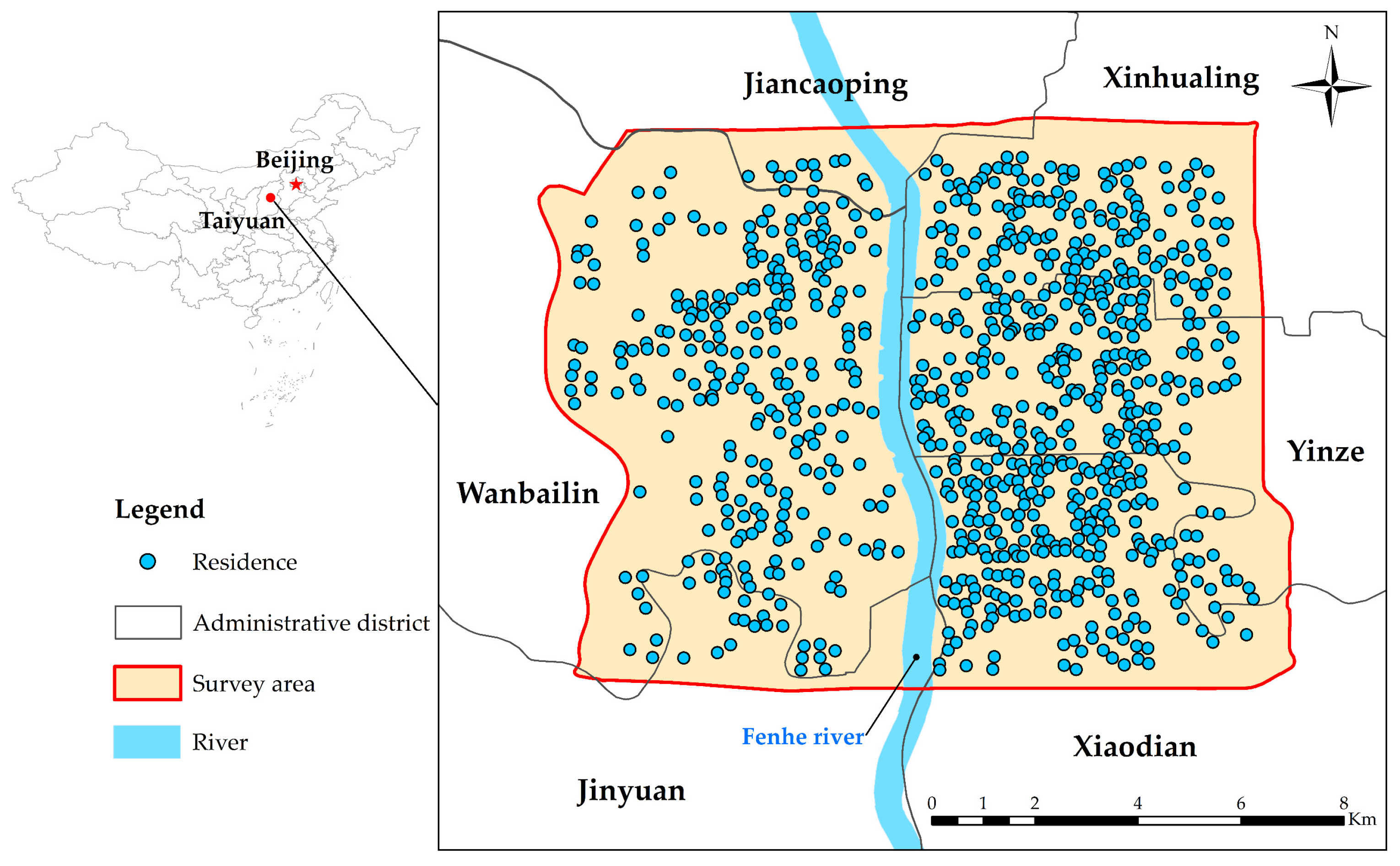
Figure 1. Survey area.
Sustainability 14 13927 g001
Figure 2. Spatial distribution of the weekly trip frequency among older adults.
Sustainability 14 13927 g002
Figure 3. Bandwidths of the different neighborhood built environment variables ( k = 4): (a) GWR; (b) MGWR.
Sustainability 14 13927 g003
Figure 4. Theoretical diagram of the Gaussian kernel function.
Sustainability 14 13927 g004
Figure 5. Spatial distribution of the adaptive bandwidth.
Sustainability 14 13927 g005
Figure 6. Flow chart of the back-fitting algorithm.
Sustainability 14 13927 g006
Figure 7. Spatial autocorrelation of weekly walking trip frequency.
Sustainability 14 13927 g007
Figure 8. Geospatial visualization of the regression coefficients: (a) location; (b) residential density; (c) land use mixture; (d) number of pedestrian crossings; (e) number of bus stops; (f) number of retail establishments; (g) number of restaurants; (h) number of recreation facilities.
Sustainability 14 13927 g008aSustainability 14 13927 g008b
Table 1. List of factors included in the neighborhood built environment.
FactorReference
Residential densityDing et al., 2014 [19]; Böcker et al., 2016 [17]; Cerin et al., 2017 [3]; Ma et al., 2018 [20]
Land use mixtureCerin et al., 2012 [15]; Feuillet et al., 2018 [5]; Cheng et al., 2022 [21]
Number of road intersectionsHanibuchi et al., 2011 [22]; Zhang et al., 2016 [13]; Xiao et al., 2020 [23]
Number of pedestrian crossingsEwing and Cervero, 2010 [24]; Lee and Dean, 2018 [18]
Number of bus stopsSmith et al., 2010 [25]; Ding et al., 2018 [26]; Cheng et al., 2021 [6]; Yang et al., 2022 [27]
Number of retail establishmentsNagel et al., 2008 [28]; Zhang et al., 2014 [29]; Feng, 2016 [30]; Yang et al., 2022 [31]
Number of restaurantsBarnett et al., 2017 [2]; Hou, 2019 [32]; Li et al., 2022 [33]
Number of recreation facilitiesCheng et al., 2019 [34]; Cheng et al., 2020 [35]
Number of public service facilitiesEngels and Liu, 2011 [36]; Yang et al., 2017 [37]; Hou et al., 2021 [38]
Table 2. Personal information statistics of older adults.
CategoryAmountPercentage (%)
Registered residenceRural45252.38
Urban41147.62
GenderMale44751.80
Female41648.20
OccupationEmployed14316.57
Unemployed23727.46
Retired48355.97
Household income (RMB)Less than 20,00013115.18
20,000–49,99927431.75
50,000–79,99931636.62
80,000–149,9999711.24
150,000 or more455.21
Disability degreeNone65876.25
Mild14216.45
Moderate/Severe637.30
Table 3. Neighborhood built environment.
Explanatory VariableDescriptionMeanSD 1
Residential densityNumber of residential buildings per km2 in the radial buffer zone.11.133.20
Land use mixtureLand use mixture measured by Equation (1).0.720.08
Number of road
intersections
Number of road intersections in the radial buffer zone.9.274.95
Number of
pedestrian crossings
Number of pedestrian crossings in the radial buffer zone.19.809.75
Number of bus stopsNumber of bus stops in the radial buffer zone.3.941.73
Number of retail
establishments
Number of stores, vegetable markets, and supermarkets in the radial buffer zone.8.544.69
Number of restaurantsNumber of dining rooms and food courts in the radial buffer zone.6.313.64
Number of
recreation facilities
Number of parks, spaces, and other entertainment equipment in the radial buffer zone.1.221.03
Number of public-service facilitiesNumber of medical care, banks, and telecommunication in the radial buffer zone.4.322.48
1 SD = standard deviation.
Table 4. Collinearity diagnosis of the explanatory variables.
Explanatory VariableFirst Collinearity DiagnosisFinal Collinearity Diagnosis
ToleranceVIFToleranceVIF
Residential density0.4252.3520.4312.323
Land use mixture0.5561.7980.5561.798
Number of road intersections0.2034.935
Number of pedestrian crossings0.1656.0520.4972.011
Number of bus stops0.6721.4880.6721.488
Number of retail establishments0.2723.6810.2723.678
Number of restaurants0.3073.2610.3083.243
Number of recreation facilities0.3682.7170.3682.717
Number of public service facilities0.4342.3050.4352.300
Measurement standardTolerance > 0.2; VIF < 5
Table 5. Comparison of the results of the model indices.
Model IndexOLSGWRMGWR
R 2 0.7490.9400.962
Adjusted R 2 0.7460.9190.949
AICc1276.952634.493235.550
Residual sum of squares216.74751.74332.930
Table 6. Comparison of the results of the model scales.
Explanatory VariableBandwidth
GWRMGWR
Location 17143
Residential density7146
Land use mixture7143
Number of pedestrian crossings7143
Number of bus stops7148
Number of retail establishments7143
Number of restaurants7143
Number of recreation facilities71862
Number of public service facilities71862
1 Location represents the intercept of the model.
Table 7. Statistical description of the regression coefficients.
Explanatory VariableMeanSD 1MinimumMaximum
Location−0.0560.257−0.6530.710
Residential density0.1420.186−0.3940.527
Land use mixture0.0780.106−0.2850.409
Number of pedestrian crossings0.1910.190−0.4500.655
Number of bus stops0.0350.092−0.2050.298
Number of retail establishments0.2350.146−0.1170.583
Number of restaurants0.1720.091−0.0940.381
Number of recreation facilities0.0570.0030.0540.064
Number of public service facilities0.0240.0020.0210.027
Adjusted   R 2 0.949
1 SD = standard deviation.
Publisher’s Note: MDPI stays neutral with regard to jurisdictional claims in published maps and institutional affiliations.