Application of Artificial Intelligence in PV Fault Detection

Abstract

The rapid revolution in the solar industry over the last several years has increased the significance of photovoltaic (PV) systems. Power photovoltaic generation systems work in various outdoor climate conditions; therefore, faults may occur within the PV arrays in the power system. Fault detection is a fundamental task needed to improve the reliability, efficiency, and safety of PV systems, and, if not detected, the cost associated with the loss of power generated from PV modules will be quite high. Moreover, maintenance staff will take more time and effort to fix undetermined faults. Due to the current-limiting nature and nonlinear output characteristics of PV arrays, fault detection is not that easy and the application of artificial intelligence is proposed for the sake of fault detection in PV systems. The idea behind this approach is to compare the faulty PV module with its accurate model (factory fingerprint) by checking every PV array’s I–V and P–V curves using the Artificial Neural Network (ANN) logarithm as a subsection of the Artificial Intelligence’s (AI) techniques. This proposed approach achieves a high performance of fault detection and gives the advantage of determining what type of fault has occurred. The results confirm that the proposed logarithm performance becomes better as the number of distinguishing points extend, providing great value to the Solar PV industry.

1. Introduction

Renewable energy sources are now playing an important role in electrical generation systems. Among them, photovoltaic (PV) systems undoubtedly constitute one of the most promising renewable green energy technologies since they allow the conversion of solar energy into electrical energy. Thus, these systems can be an ideal solution for covering the basic energy needs of contemporary and next-generation societies [1]. The number of Photovoltaic (PV) systems installed around the globe has been exponentially increasing. Since the year 2000, the global cumulative solar photovoltaic capacity has been steadily increasing. Global solar PV capacity was 773.2 gigawatts in 2020, with 138 gigawatts of additional PV capacity installed in the same year [2].

The protection of PV systems has been less investigated. The arrays and relevant wiring of PV systems are outdoor components and, therefore, experience harsh environmental conditions. This makes them susceptible to different faults and abnormal situations. However, the protection of the arrays has some challenges [3].

1.1. Background

Various factors, including maximum power point tracking error, environmental effects like shading and dust or snow buildup on the PV surface, wiring losses and aging, and malfunction in other PV components like the power conditioner unit and the inverter can all have an impact on how well a PV system operates. According to a monitoring study in [4], faults may cause a PV system to generate roughly 18.9 percent less power annually. In order to continually analyze the current, voltage, and output power characteristics of a PV system and find both existing and emerging defects, proper techniques have to be developed.

Table 1. Comparative analysis of external factors on the performance of PV systems [5].

NO	Factors	Nature	Effect on Power Output	Efficiency
1	Irradiation	Variable	Increase	Increase
2	Temperature	Variable	Decrease	Decrease
3	Dust	Variable	Decrease	Decrease
4	Shading	Constant	Decrease	Decrease
5	Angle of tilt	Constant	Depends	Depends
6	Wind velocity	Variable	Depends	Depends
7	Humidity	Variable	Decrease	Decrease
8	Color spectrum	Constant	Variable	Variable
9	Mounting	Constant	Depends	Depends
10	Cable thickness	Constant	Increase	Increase

summarizes how the output power and the efficiency of the PV system be affected by outdoor factors.

1.1.1. Types of Faults in the PV Systems

When there is a decrease in the output power of the PV arrays compared to what it is expected to be, the most common faults in photovoltaic arrays are identified. It could be due to a fault in a PV module or string of PV modules, such as shadowing, soiling, and snow cover, deterioration and corrosion, by-pass or shunted diode failure, or degradation and corrosion [6]. The faults shown in

Table 2. Classification of faults in the DC side of the PV systems [7].

Side	Factors	Nature
DC	Mismatch faults	Partial shading
		Uniform irradiance distribution
		Soiling
		Snow covering and hot spot
	Earth fault	Upper ground fault
		Lower ground fault
	Arc fault	Series arc fault
		Parallel arc fault
		Line-to-line faults
		Bypass diode faults
		Degradation faults
		Bridging fault
		Open-circuit fault
		MPPT faults

can also be caused by poor electrical connections, short circuits, or wire losses. Sometimes the faults occur in the AC side of the PV system as listed in

Table 3. Classification of faults in the AC side of the PV systems [7].

Side	Factors	Nature
AC	Inverter faults	Failure in IGBTs, capacitors, and drive circuitry can result in inverter failure
	Sudden natural disasters	Lightning and storm

.

1.1.2. PV Fault Detection

To clear the faults in the AC side of the PV system, existing AC protection schemes for distribution systems are easily employed and fault clearance can be achieved. However, in the DC side of the PV systems, due to the unpredictable nature of the PV output power generation, various challenges still exist for fault clearance.

In general, PV fault detection methods make it possible to pinpoint the kind and location of various PV system faults. Such methods ought to be strong in order to increase system lifetime and reliability and offer safe functioning. In order to prevent consequences and additional failures, the procedures also need to be quick in spotting evolving faults. The methods are divided into six major categories: electrical methods, machine learning methods, visual methods, imaging solutions, and ARC fault detectors [6].

The performance and efficiency of PV panels are affected by a number of factors, including irradiance, temperature, humidity, wind speed, dust, rain, snow, shade, cell breakdown, and age. As a result, it is challenging to specify specific fault detection boundaries. Machine learning techniques can be utilized to create self-learning systems and get over that limitation because they have the capacity to automatically learn and adjust to specific conditions from a given set of data [8].

1.2. Related Workes

The majority of fault detection systems in the DC side of a PV plant can be classified into one of the methods described in this section as shown in Figure 1. These methods differ in terms of the types of faults detected, the types of measurement sensors required, the most practical application for the proposed method, and the method used to generate the test results, such as whether a simulated computer-aided method or purely experimental validation was performed to present the results.

Direct difference measurement between expected and measured current, voltage, or power (DDM) is based on predicting PV parameter values under various environmental conditions and comparing real-time measurements to these predicted values. Typically, these strategies set thresholds below or above the point at which failure signals appear. For example, in [9], the PSIM software package was used to create a simulation model of a photovoltaic (PV) system. Thereafter, a 3-kW photovoltaic (PV) system was installed. The model created by PSIM with series and parallel connections was used not only for fault analysis but also to represent the I–V and P–V characteristics of the fault at various surface temperatures and isolations during normal operation. Finally, in order to identify the faulting types of a 3 kW PV system, a novel extension diagnosis approach based on the extended correlation function and the matter–element model was introduced. The proposed PSIM-based PV module possessed a higher accuracy in electrical parameters than the conventional mathematic model. Furthermore, the simulated results also emphasized that the proposed fault diagnosis method could easily recognize the main fault category and indicate the possibilities of others. In [10], this study proposed and implemented a method for detecting the number of open and short circuit faults and distinguishing them from partial shading situations. Only the operating voltage of the PV string and the ambient temperature were measured. This method had been successfully validated experimentally using a PV array formed by 8 × 3 PV modules. One more example of the DDM technique is to be found in [11]. In this study, a monitoring system that provided real-time voltage and current readings for each PV module was studied. The performance of a fault detection algorithm formulated as a clustering problem and addressed using the robust minimum covariance determinant (MCD) estimator was evaluated on simulated arc and ground faults. The algorithm was found to perform well on many types of faults commonly occurring in PV arrays.

The second method is the adjacent String Comparison Measurement Technique (ACMT). With this method, the differences in measurements from nearby strings are utilized as a reference for finding faults in the PV string. They are only suitable for PV farms with string inverter systems. As an example of ACMT, the ACMT technique was used in [12] and was found to reduce failure misjudgment and improve failure judgment accuracy by comparing the current output measuring value of the suspected faulted cell module group to that of the surrounding group. Another paper using the ACMT method is [13] wherein a sensor was used to collect the electric current and voltage signal of each series branch. The difference between the maximum current value and the other values was then used to determine the fault. The faulty solar series branch could then be determined by calculating the deviation of each branch. It could determine the fault section in the branch based on the voltage signal. Finally, a failure notification was generated for the maintainer’s immediate attention. The ACMT method has one more advantage in that it does not require weather measurement. For fault detection based on instantaneous PV string current, outlier detection rules have been proposed in [14]. Three rules were discussed in detail in this paper: the 3-Sigma rule, the Hampel identifier, and the Boxplot rule. The Hampel identification and the Boxplot rule were shown to be effective in detecting PV faults. Furthermore, as the number of PV measurements increased, the proposed models became more reliable. For real-time operation, the described approaches might be combined with a PV monitoring system.

The energy losses in the PV system are the basis for The Energy Loss Analysis (PELA) strategy. The rate of energy losses in the PV system is used for fault classification and detection. The authors in paper [15] proposed a detection method based on comparing the estimated production (tension, current, and the inverter’s power) with the actual production. The day’s climatic data (irradiance and temperature) allowed the authors to determine the amount of production. Other authors in [16] proposed a system that allowed for the module-level monitoring of PV plant characteristics such as voltage and current at the working power point. Using these parameters, a Matlab prototype diagnosis tool was created and it was experimentally confirmed in a real rooftop PV generator by introducing various faults. Fixed object shading, localized dirt, generalized dirt, probable hotspots, module degradation, and excessive losses in DC cables were among the issues that the tool can diagnose. Another example of the PELA technique was used for small grid-connected PV systems. A completely automated performance check had been created by [17] in order to ensure maximum energy yields and to optimize system maintenance. The goal was to detect system failures and changing operating conditions early on in order to save energy and money for the operator. The approach was created using satellite-derived solar irradiance data to replace on-site measurements. The expected energy yield of a PV system was calculated using a simulation model. Finally, an automated failure detection method searched for the most likely failure sources and warned the operator if a defined difference between the simulated and actual energy yield occurred.

For fault identification and categorization, the fourth method employs machine-learning techniques. Machine-learning techniques are used to better understand the relationship between the PV system’s input and output characteristics, and then the trained models are utilized to detect and categorize faults. Some of the machine-learning techniques used so far are: paper [18] presented the emerging kernel-based extreme learning machine (KELM) in order to automatically establish the fault diagnosis model. Whereas the input of the fault diagnosis model was proposed based on the key points and model parameters extracted from monitored I–V characteristic curves and environment conditions. Fault experiments were carried out on both the laboratory PV array and the PV model in order to acquire abundant simulated and experimental fault data samples. Finally, KELM was applied to train the fault diagnosis model using the data samples. In addition, the authors in [19] provided a fault detection technique based on a study of theoretical curves that describe the behavior of a PV system in use. Virtual instrumentation (VI) LabVIEW software was used to simulate a number of properties such as voltage ratio (VR) and power ratio (PR). Furthermore, the detection limits were compared to data collected from a 1.1 kW PV system at the University of Huddersfield in the United Kingdom. A fuzzy logic classification system with two inputs and one output was used to process samples that were outside of the detection limits. Different methods of MLTs were used as follows: modified ANN with the extension theory [20], evidence theory and Fuzzy mathematics [21], TSK-FRBS Fuzzy estimator [22], Bayesian belief networks [23], three-layered ANN [24], decision tree-based method [25], and graph-based semi-supervised learning [26].

In the event of a fault, the temperature of the PV module will fluctuate. Heat Exchange and Temperature-Based Models (HETM) approach the use of the heat exchange and module temperature during a faulty situation in order to detect and classify faults. In paper [27], two working points on the PV module, as well as the associated temperature from a thermal camera, were used to calculate essential parameters such as total effective solar energy, total heat exchange coefficient, and ambient temperature. A fault diagnosis method based on the generated model was demonstrated using the model. Finally, experiments were used to validate the model. The authors in [27,28] used the thermal behavior of PV cells caused by electrical faults to model the physical defects of various types of PV cells.

External Injection Method (EIM) approaches depend on external equipment such as signal generators and LCR [inductance (L), capacitance (C), and resistance (R)] meters. To detect and/or characterize the type of faults in the PV system, the response of the PV system to the injected signals is considered. As an example of the use of the EIM technique, the authors in [29,30] compared the input signal to the PV cell, module, or string to the reflected signal from the circuit. The failure point in the line and the type of failure were determined by the signal delay and waveform shape change.

1.3. Scientific Contribution

Over the last decade, solar energy has become increasingly popular as a source of electricity and heat. Photovoltaic (PV) systems, in particular, have established an important role in the electricity energy sectors, contributing to more than 10% of the total power supply today. Grid-connected PV systems are becoming more popular for a variety of reasons, including low installation costs, quick energy, and investment payback, which may include customer incentives. In this case, continuous output energy production needs to be confirmed in order to satisfy the cost-benefit analysis of PV installations [31]. Fault conditions, like those in other power production systems, are unavoidable in PV systems and will be one of the most difficult problems to tackle. Maintaining system reliability and reducing power and energy losses are examples of such difficulties. Failures in the solar cell panel and system components, such as power converters and wiring connections, can be defined as faults in off-grid, on-grid, and hybrid power systems [32]. The main contribution of this paper is the presentation of an Artificial Intelligence technique that has the ability to detect and classify the faults in the DC side of the PV system based on the voltage, current, and outpower curves. Although there are several methods utilized to achieve the same purpose, the AI technique has high accuracy, quick detection, and classification advantages. In this paper, the model was designed based on real data gathered from a weather station located at King Saud University, Kingdom of Saudi Arabia. The most frequent faults in the DC side of the PV system were considered. Three models depending on the Artificial Neural Networks (ANN) configuration were built. The three models achieved high accuracy of detection and classification when compared to the other techniques. The proposed approach will save time and effort for maintenance as well as the cost of sudden power reduction.

The structure of the article is as follows: a brief introduction about the PV system, the background of the factors which affect PV system production, the fault detection problem and its related techniques, and the scientific contribution are provided in Section 1. The methodology, which includes the data-gathering stage, modeling, and fault simulation, is provided in Section 3. Section 4 presents the results and their discussion. Finally, in Section 5, the conclusions of the study are introduced.

2. Methodology

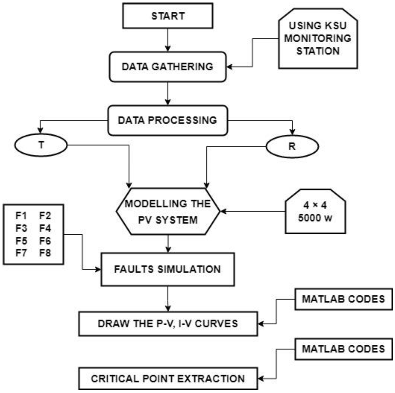
The flowchart of processes that passed through is introduced in Figure 2. In addition, each subsection will clarify the stages starting with the data-gathering stage, passing through the system modeling stage, the fault simulation stage, and, finally, the AI model configuration stage. Matlab and Simulink were utilized to build a 5 kW PV system and simulate the studied faults.

2.1. Radiation and Temperature Data Gathering

Radiation (R) and Temperature (T) affect the output production of the PV system. In order to have an accurate simulation of the PV system, radiation and temperature have to be monitored using accurate devices. In this subsection, the strategy followed to monitor radiation and temperature is explained in addition to the monitoring station specifications.

King Abdullah City for Atomic and Renewable Energy (K.A.CARE) is the sponsor for all the monitoring stations around the Kingdom of Saudi Arabia (KSA). In this paper, King Saud University (KSU) station was utilized for monitoring the needed data.

King Saud University (KSU) has a modern station that was created to monitor weather conditions such as wind speed, wind direction, direct normal radiation, global horizontal radiation, diffuse horizontal radiation, station pressure, humidity, and air temperature. The station registers one reading per minute. This operation continues throughout the year. The main information about the monitoring station is provided in

Table 4. Basic Station Information.

-	Information
Station name	King Saud University Solar Monitoring Station
City	Riyadh
Latitude (N)	24.72359 degrees
Longitude (E)	46.61639 degrees
Station Elevation (A.S.L)	688 m
Station Host	King Saud University
Station Power Source	PV
Operating Since	1 November 2014
Location	Roof

.

Temperature and radiation are the inputs for the PV system.

Table 5. Date, time of monitoring, and the number of readings.

-	Information
Date of monitoring	12 January 2021–14 January 2021
Time of monitoring	11:00 a.m.–01:59 p.m.
No. of radiation readings	570
No. of temperature readings	570

illustrates the preprocessing operation of the monitored data. The data was chosen at a time over the year according to specific criteria. The gathered data was used after processing to simulate the healthy and faulty PV system. The dates and the times of monitoring were chosen based on the following criteria:

• The monitored radiation and temperature have to be close to the ideal conditions (T = 25 °C, R = 1000 w/m²);
• The irregular data or noisy ones (which occur due to devices’ reading failure) should be excluded and replaced with fit ones;
• As the samples of the gathered data increase, the PV model will spend more time for simulation. So, they were kept suitable.

2.2. PV Sytem Modelling

2.2.1. PV Module

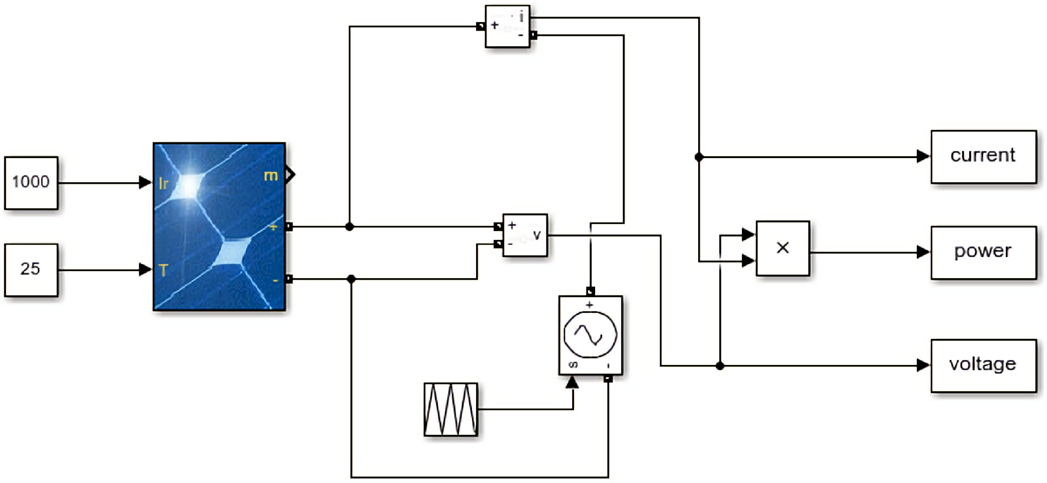
Simulink provides great features that enable users to simulate such physical systems. A solar panel can be simulated as well. A PV solar panel has two inputs, which are radiation (R) and temperature (T). The output voltage (P), current (I), and voltage (V) are worked out. Moreover, the P–V relation and the I–V relation can be plotted and these curves change by changing the weather conditions.

Figure 3 shows the single module configuration and this is used to plot the P–V and I–V curves.

Table 6. PV module characteristics.

PV Module Characteristics	Name
Module	Jenko Solar JMK310-M72
PV Module Data	Value
Maximum Power (Pmax)	309.925 W
Open Circuit Voltage (Voc)	47.1 V
Short Circuit Current (Ish)	8.78 A
Voltage at maximum power point (Vmp)	38.5 V
Current at maximum power point (Imp)	8.05 A
Cells per module	72

illustrates the characteristics of the simulated PV module. These characteristics differ from one module to another.

2.2.2. PV System

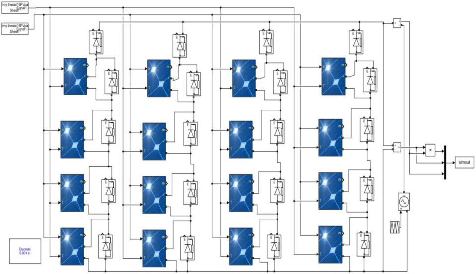
PV systems have a high output capacity in real life. This can be achieved by connecting more than one module. Connecting solar panels increases the voltage and the current of the whole system and, subsequently, the total output power will maximize. A series connection of solar panels can improve the voltage of the system. Moreover, the current can be increased by connecting panels in parallel. In this paper, a PV system of 5000 W is simulated using Simulink software 2019b. All characteristics of the PV system are illustrated in

Table 7. PV system characteristics.

PV System Data	Value
Maximum Power (Pmax)	5000 W
Open Circuit Voltage (Voc)	188.4 V
Short Circuit Current (Ish)	35.49 A
Voltage at maximum power point (Vmp)	154 V
Current at maximum power point (Imp)	32.2 A

.

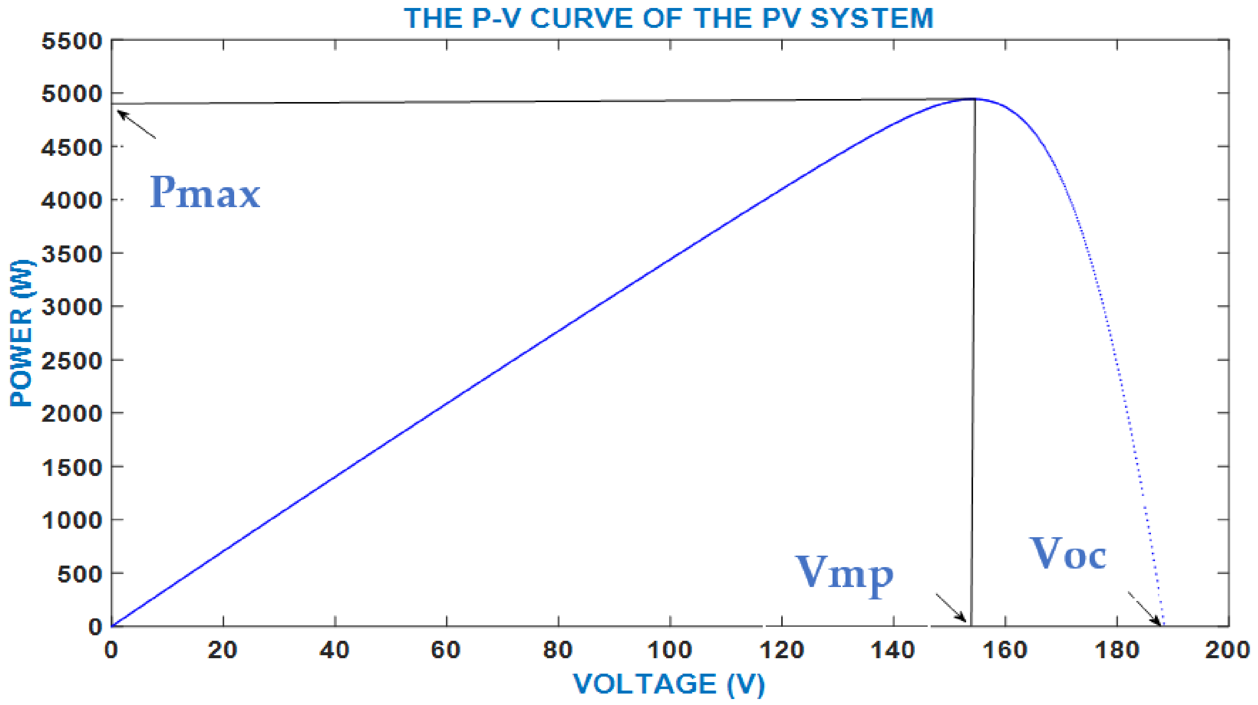
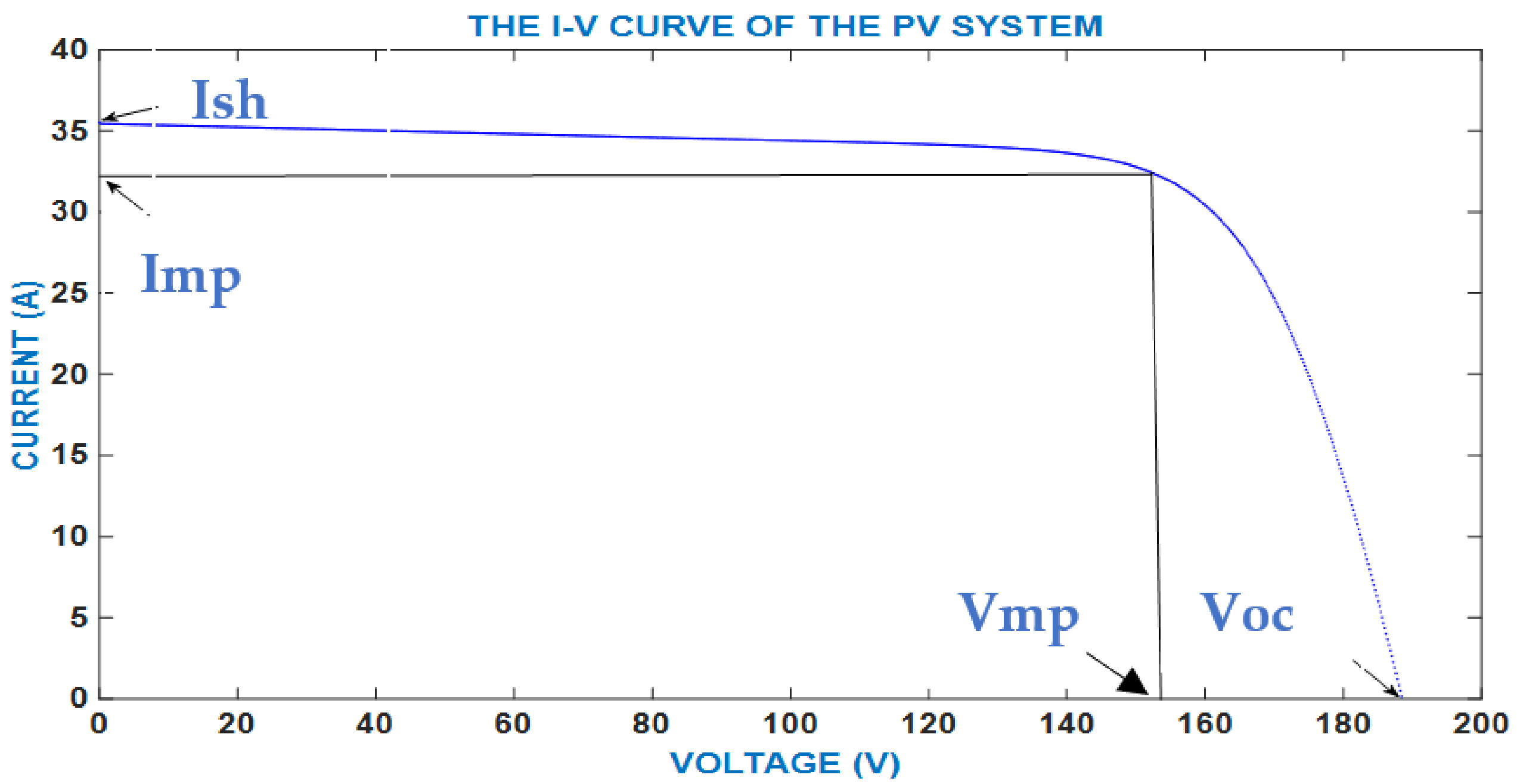
Figure 4 shows the proposed model for the PV system. The output of the PV system is simulated in order to plot the P–V and I–V curves. These curves are important to check whether the system suffers from a fault or not. Their importance will also help later on in order to differentiate between the types of faults. Figure 5 and Figure 6 show these important curves.

There are critical points in the P–V and I–V curves of the PV system. These are necessary in order to differentiate between the different types of faults. These points are the maximum power (Pmax), open circuit voltage (Voc), short circuit current (Ish), Voltage at maximum power (Vmp), and current at maximum power (Imp).

2.3. Fault Simulation

The output power, voltage, and current corresponding to each reading of temperature and radiation registered in the data-gathering phase are now generated using the model in Figure 4. The most frequent faults in the DC side of the PV system (illustrated in

Table 8. The most frequent faults in the DC side of the PV system.

Fault Type	Symbol 1
No Fault	F1
Partial Shading Fault	F2
Line-to-Line Fault	F3
Open Circuit Fault	F4
Degradation Fault	F5
Bridge Fault	F6
Bypass Diode Fault	F7
Hybrid Fault 2	F8

¹ Assumed in order to address the fault symbols F1–F8. ² The Hybrid Fault is assumed to have F3 and F5 when they occurred at the same time.

) are simulated one by one using the Simulink software using the configurations of faults illustrated in

Table 9. PV system configuration of each fault.

Fault Type	Symbol	PV System Configuration
No Fault	F1	Figure 4
Partial Shading Fault	F2	Full or partial-shaded panels can be simulated by decreasing the radiation as input
Line-to-Line Fault	F3	Low-resistance connection between two sites of differing potential in the same string
Open Circuit Fault	F4	Breakdown of panel–panel cables or joints
Degradation Fault	F5	An increase in series resistance between the modules
Bridge Fault	F6	Low-resistance connection between two sites of different voltage in different strings
Bypass Diode Fault	F7	This type of fault can be simulated by shorting the bypass diode across the module.
Hybrid Fault	F8	Two types of faults occur at the same time

. The PV system generates different output values of the power, voltage, and current according to the input radiation and temperature and the type of fault. By using these findings, the P–V and I–V curves are plotted. Then, they are compared with healthy case curves (No Fault status).

The Extracted Results from the Fault Simulation

The PV model provides a result at each moment. Corresponding to each temperature (T) and radiation (D) that the system reads as inputs, voltage, current, and power result. Codes using Matlab are generated to plot the P–V and I–V curves.

Table 10. The extracted results from the fault simulation.

Critical Point	Symbol	Shown in
Maximum power	Pmax	Figure 5 and Figure 6
Open circuit voltage	Voc	Figure 5 and Figure 6
Short circuit current	Ish	Figure 6
Voltage at maximum power	Vmp	Figure 5 and Figure 6
Current at maximum power	Imp	Figure 6

shows some critical points in the generated curves that are also extracted using Matlab codes.

2.4. Formulation of AI Logarithm Inputs

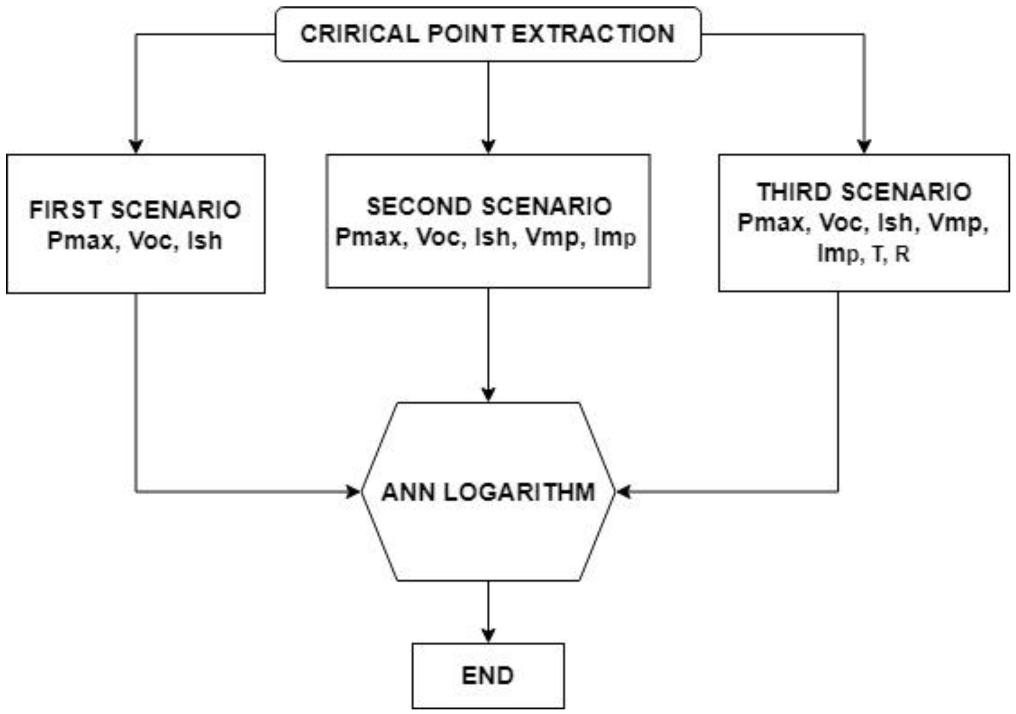
This stage comes after the data has been collected and the faults have been simulated in the PV model. The maximum power (Pmax), open circuit voltage (Voc), short circuit current (Ish), the voltage at maximum power (Vmp), and the current at maximum power (Imp) were used to formulate the AI logarithm. The flow chart in Figure 7 illustrated these processes.

Artificial Neural Networks as Part of Artificial Intelligence

An Artificial Neural Network (ANN) as a kind of Artificial Intelligence (AI) is applied to the PV system output curves in order to detect and classify the faults in the DC side of the PV system.

The ANN logarithm passes through several processes. First, logarithm training. In this phase, the data is collected before it is used in order to train the ANN logarithm so that the inputs and outputs should be identified. The logarithm’s role is to find the relationship between the given inputs and outputs. Second, validating. In the beginning, the data should be divided into three groups for three purposes (training, validating, and testing). The validating data is used to validate the relationship between the inputs and the outputs created in the first phase and then an attempt is made to enhance this relationship until the best connection is reached. Finally, the testing phase. This phase is used to measure the logarithm’s performance.

Three scenarios of ANN application in the PV system for fault detection will then be introduced. The three scenarios differ from each other by the number of inputs. The three scenarios are then tested in order to ascertain the best detection and classification performance.

The ANN logarithm has to be trained using previously collected data. Three scenarios were created according to the number of inputs which were: the maximum power (Pmax), the open circuit voltage (Voc), the short circuit current (Ish), the voltage at the maximum power (Vmp), the current at maximum power (Imp), radiation (D), and temperature (T). It is identified in the previous section how these parameters were extracted from the P–V and I–V curves. Figure 8 shows the logarithm configuration and

Table 11. Results of fault simulation for three scenarios.

Purpose	Number
Total Data	4560
Training Data (75%)	3420
Validation Data (5%)	228
Testing Data (20%)	912
Inputs (First Scenario)	Imax, Voc, Ish
Inputs (Second Scenario)	Imax, Voc, Ish, Vmp, Imp
Inputs (Third Scenario)	Imax, Voc, Ish, Vmp, Imp, R, T
Output	8
Hidden Layers	10

illustrates the three scenarios’ details.

3. Results

The ANN logarithm was applied to the PV system model in order to detect and classify the faults that occurred in the DC side of the PV system. As explained in the last sections, three scenarios were created and each one had its own results. They were considered and assessed in order to check their performance in the detection and classification of PV faults. Several types of assessment techniques were used to make sure that the ANN logarithm caught the highest level of detection and classification.

Comparison between the three scenarios was investigated depending on the assessment tools. In addition, the limitations and features of each scenario were introduced. Finally, an analytical discussion of the findings was presented to decide which scenario achieved the highest performance accuracy.

3.1. Confusion Matrices

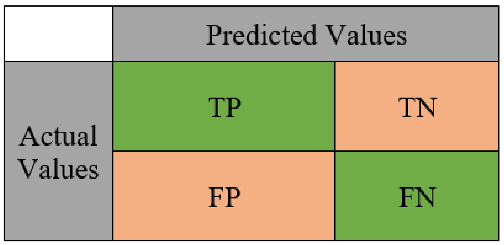
A confusion matrix is a technique used for summarizing the performance of a classification algorithm. Calculating a confusion matrix can give you a better idea of what your classification model is getting right and what types of errors it is making. The following terminologies are important to understand the overall confusion matrix [33], and there are distributed in the matrix as in Figure 9:

• True Positive (TP): You predicted positive and it was true.
• True Negative (TN)): You predicted negative and it was true.
• False Positive (FP): (Type I Error) you predicted positive and it was false.
• False Negative: (Type II Error) you predicted negative and it was false.

The following equation is important for calculating the accuracy: From all the classes (positive and negative), how many of them has the logarithm predicted correctly?

$$\mathrm{accuracy}=\frac{\mathrm{TP}+\mathrm{TN}}{\mathrm{Total}},$$

(1)

3.1.1. First Scenario

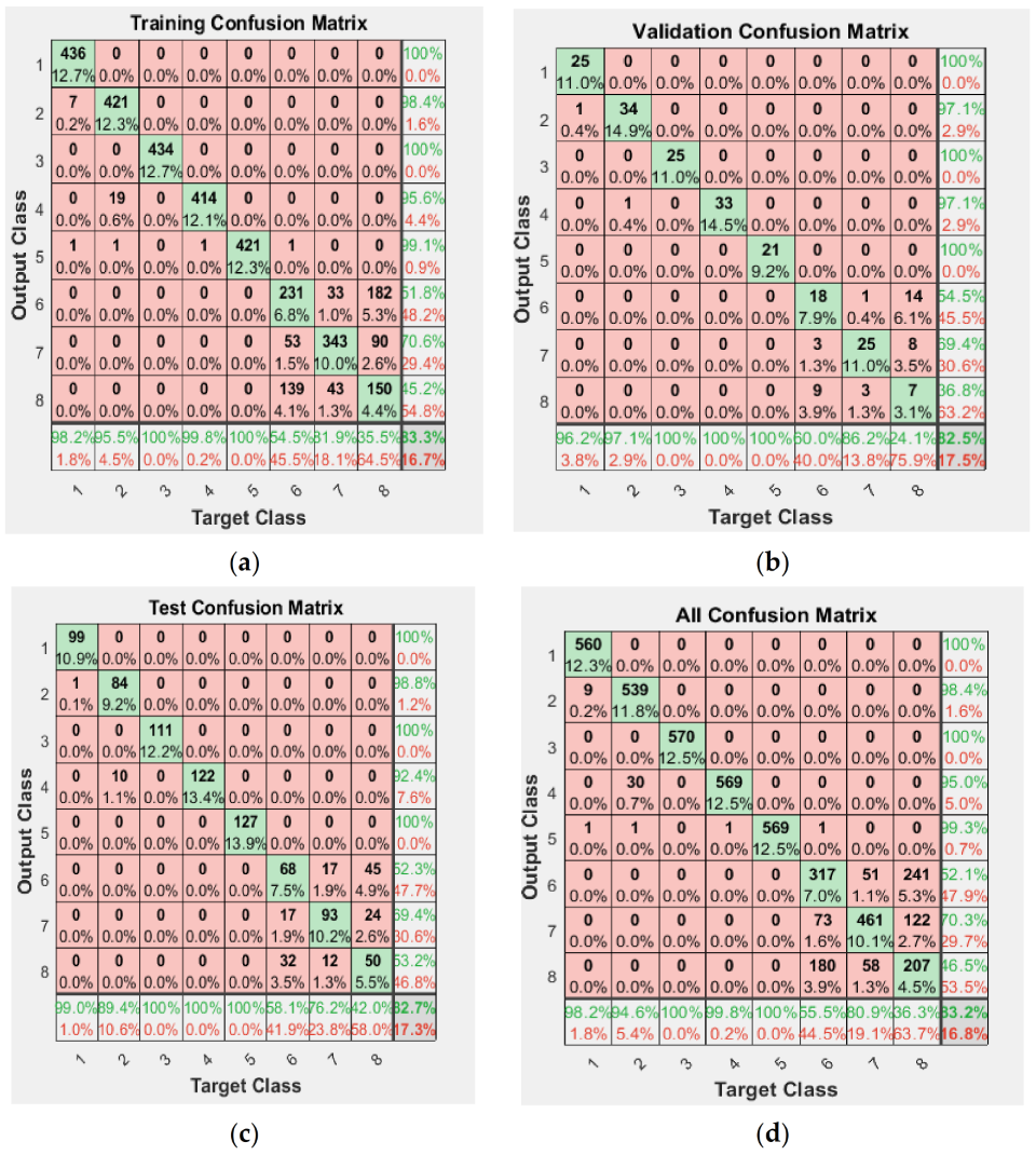
As shown in Table 11, the first scenario depends on Pmax, Voc, and Ish as the inputs of the ANN logarithm. The following confusion matrices (Figure 10) were used to assess the ANN performance.

3.1.2. Second Scenario

The second scenario was built by utilizing Pmax, Voc, and Ish as inputs to the ANN block, which were the same as the first scenario. The difference is to be found by adding two more parameters to the inputs which were Vmp, and Imp as shown in Table 11. The following confusion matrices (Figure 11) were used to assess the ANN performance.

3.1.3. Third Scenario

The new third scenario considered the temperature and radiation in addition to the previous parameters (Pmax, Voc, Ish, Vmp, and Imp) as inputs to the ANN block. The following confusion matrices (Figure 12) were used to assess the ANN performance.

3.2. Error Histogram

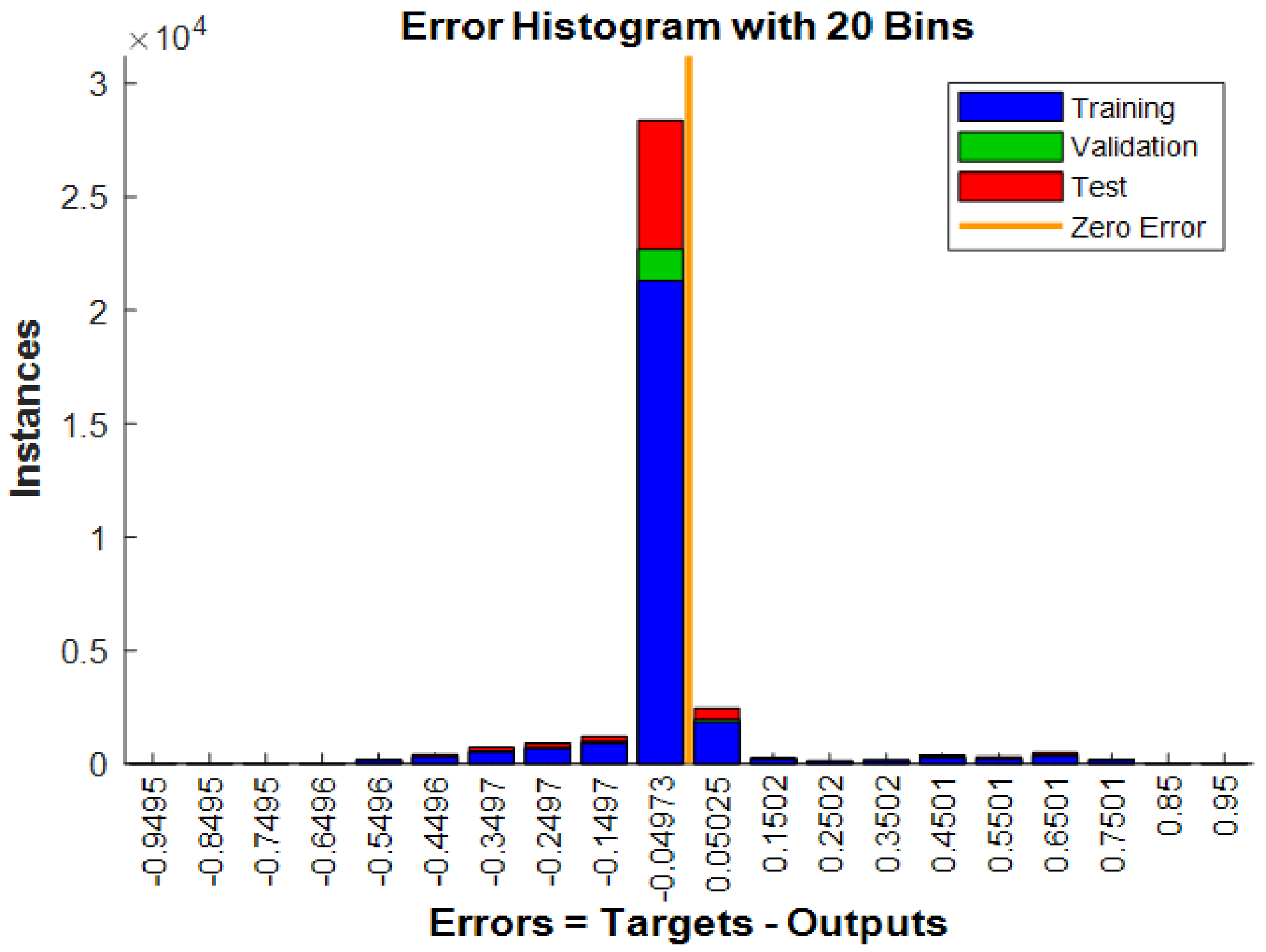
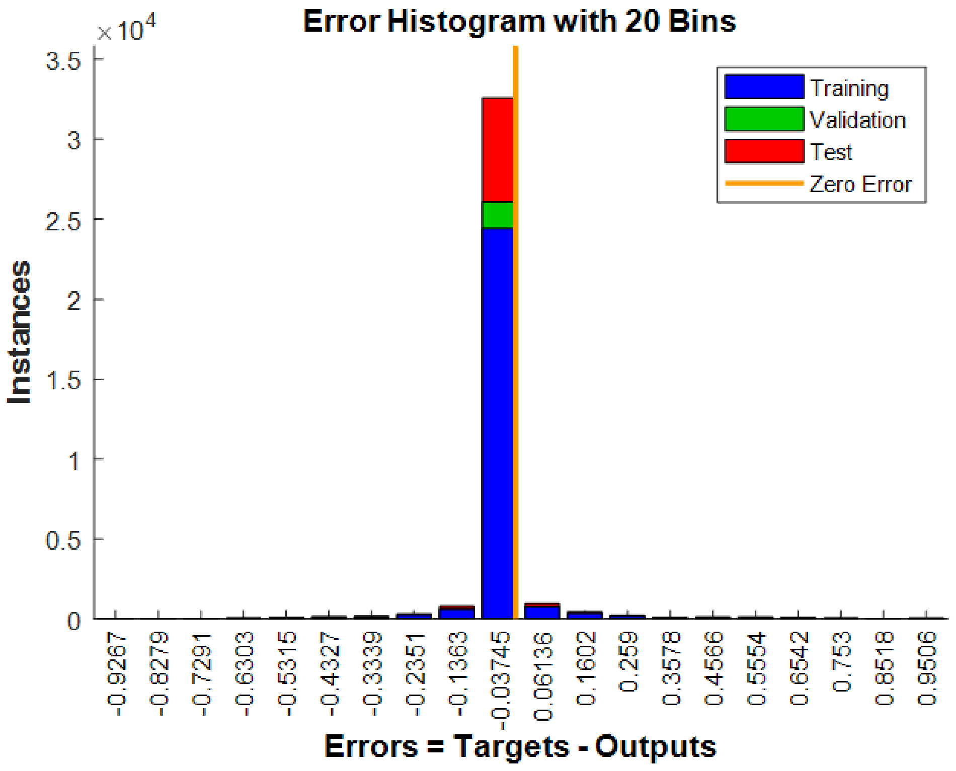
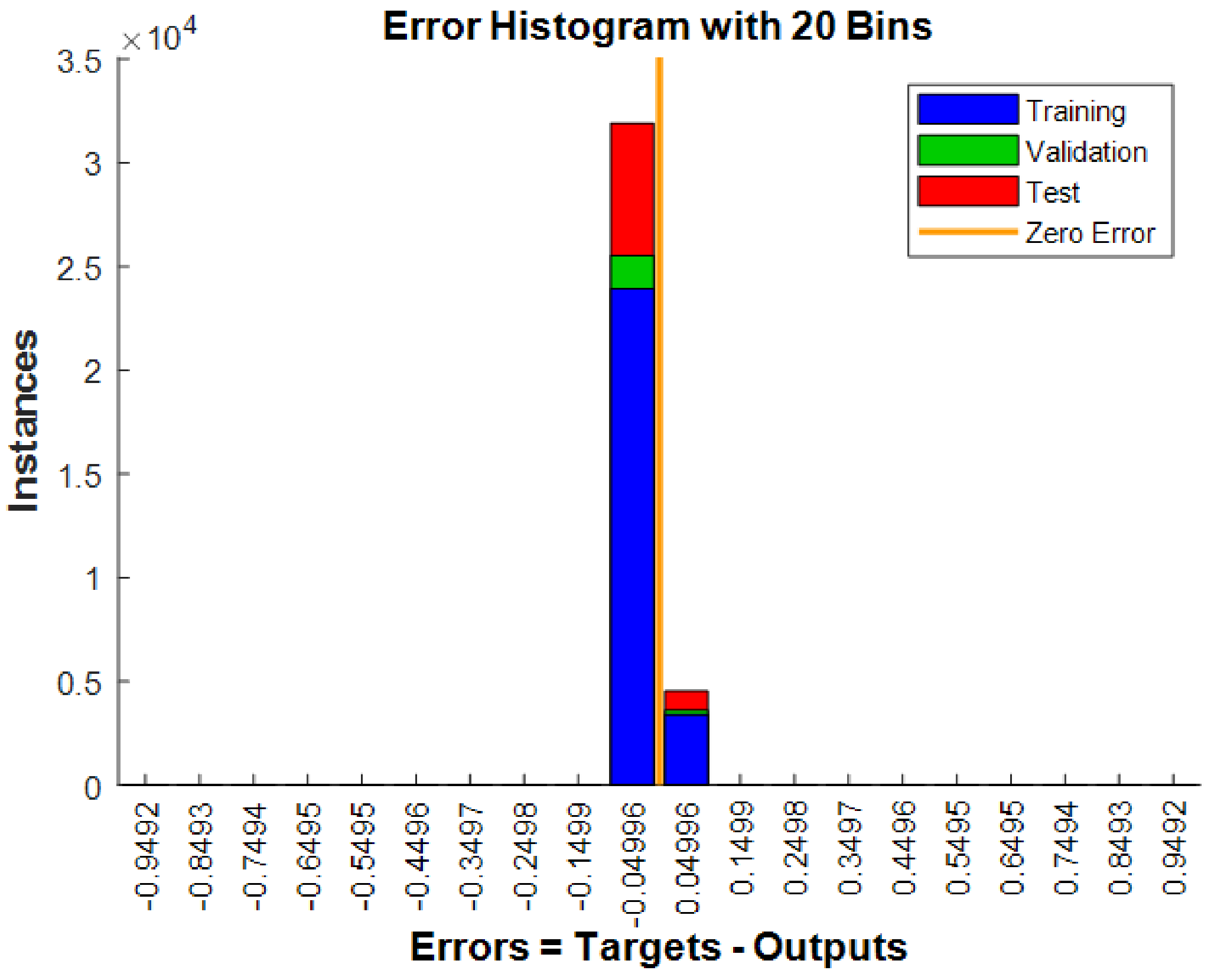
An Error histogram is the histogram of errors between the target values and the predicted values after training a feedforward neural network. Bins are the number of vertical bars that are observed on the graph (Figure 13, Figure 14 and Figure 15). The total error range is divided into 20 smaller bins. The y-axis represents the number of samples from the dataset, which lies in a particular bin [34].

3.3. Receiver Operating Characteristic (ROC)

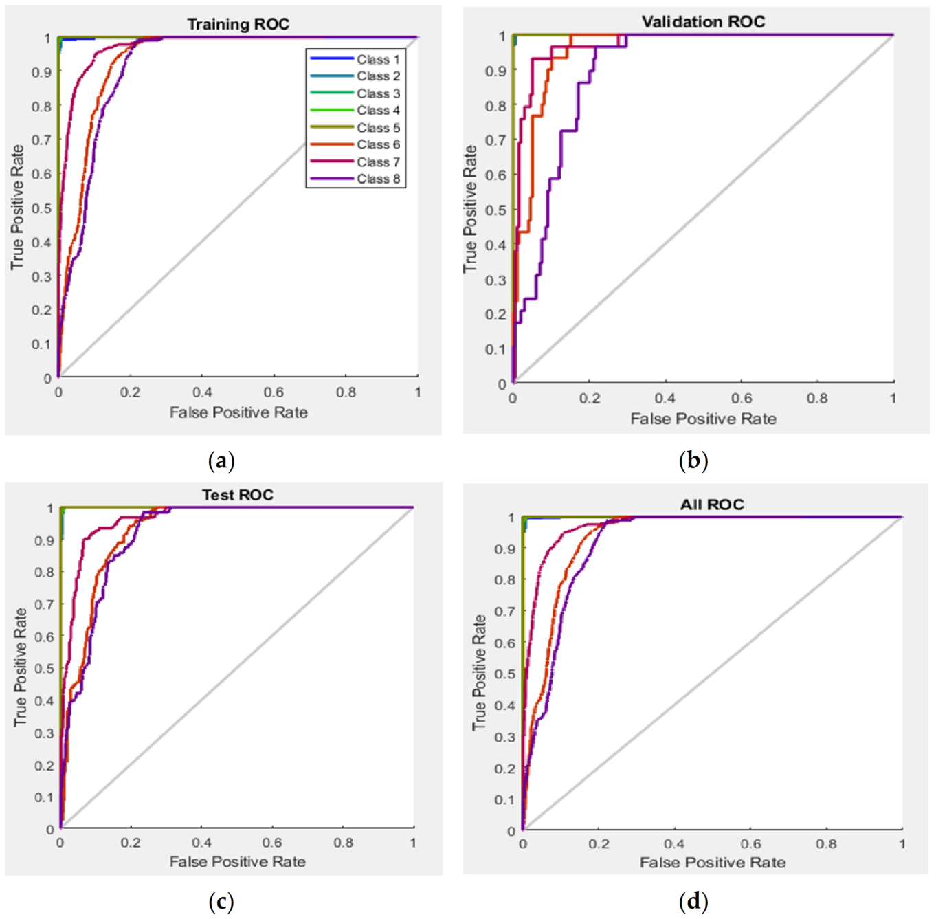
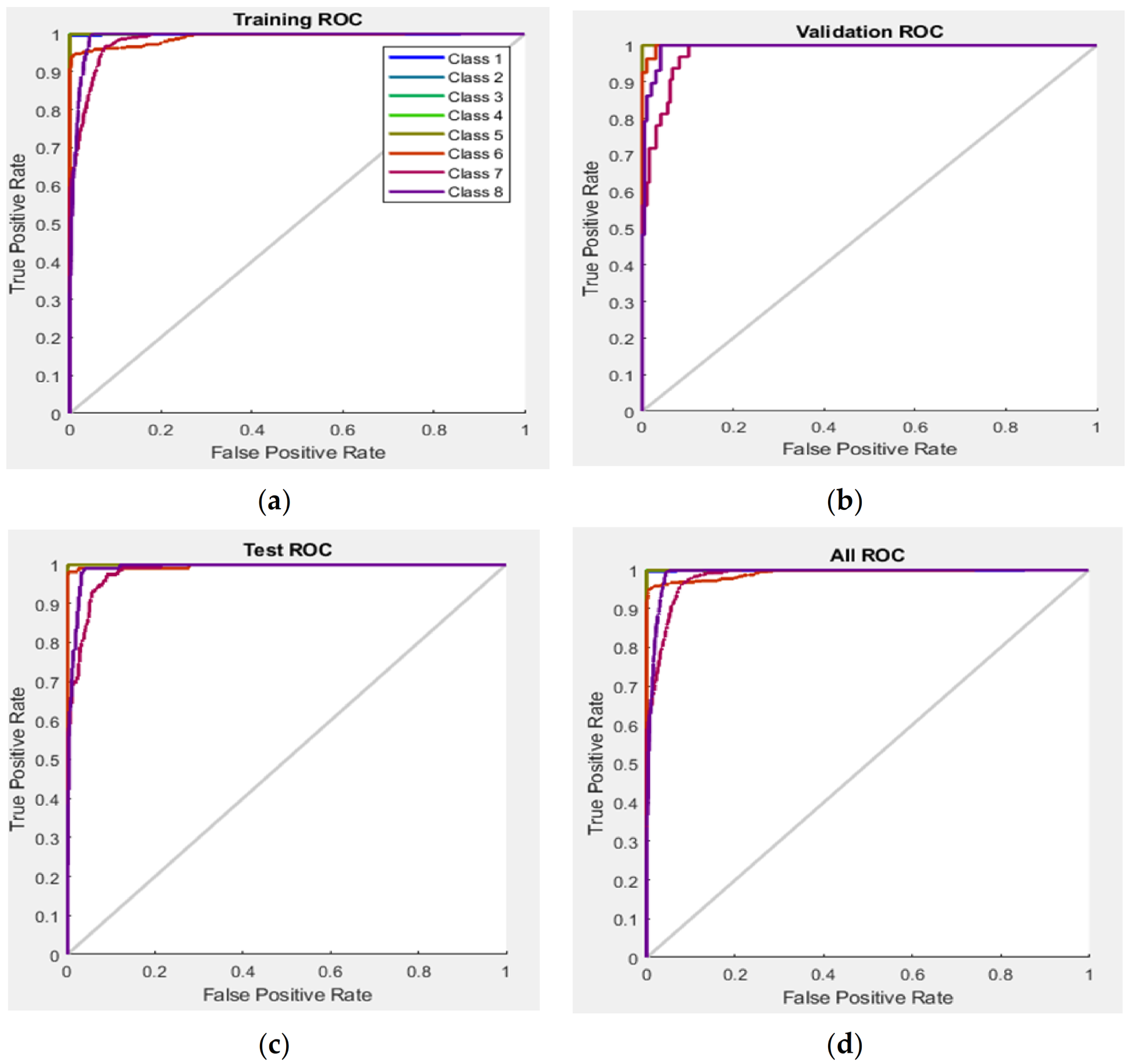
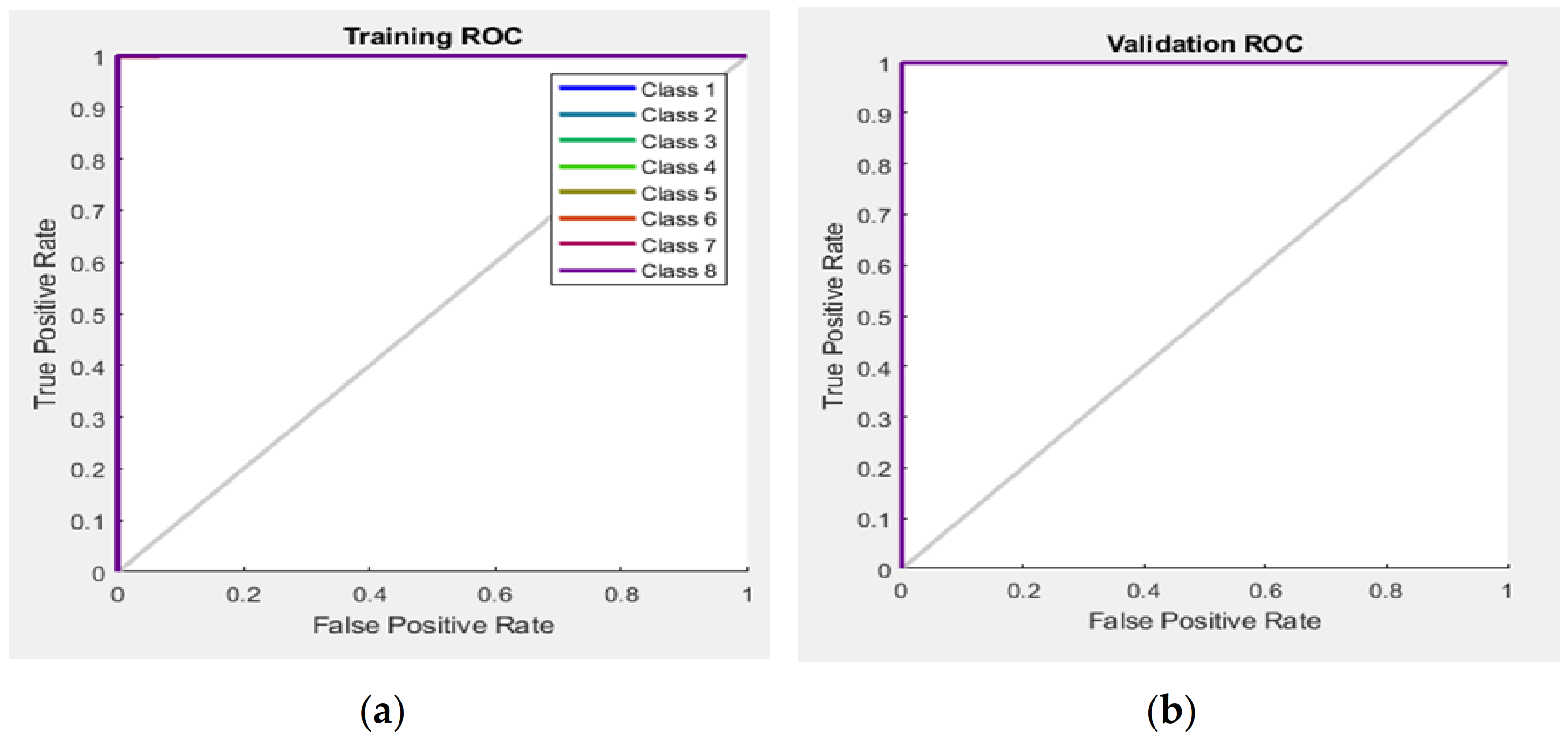
An AUC–ROC curve is a performance measurement for the classification problems at various threshold settings. ROC is a probability curve and AUC represents the degree or measure of Separability. It tells us how much the model is capable of distinguishing between classes. The higher the AUC, the better the model is at predicting 0 classes as 0 and 1 classes as 1. The ROC curve is plotted with TPR against the FPR where TPR is on the y-axis and FPR is on the x-axis. An excellent model has an AUC near 1 which means it has a good measure of Separability. A poor model has an AUC near 0 which means it has the worst measure of Separability. Moreover, when AUC is 0.5, it means that the model has no class separation capacity whatsoever [35]. The following figures (Figure 16, Figure 17 and Figure 18) illustrate the ROC curves for the three scenarios.

3.4. Best Validating Performance Plot

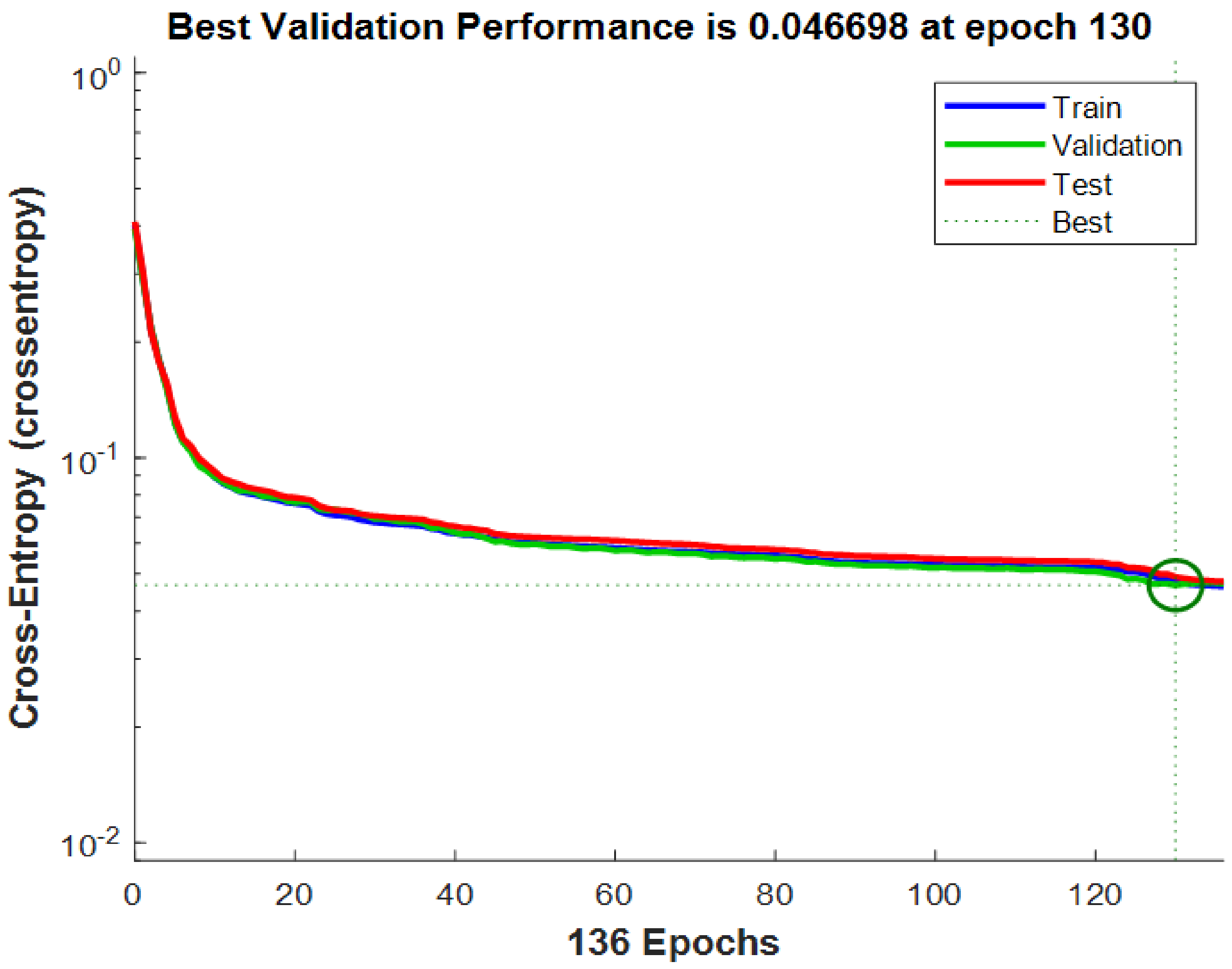
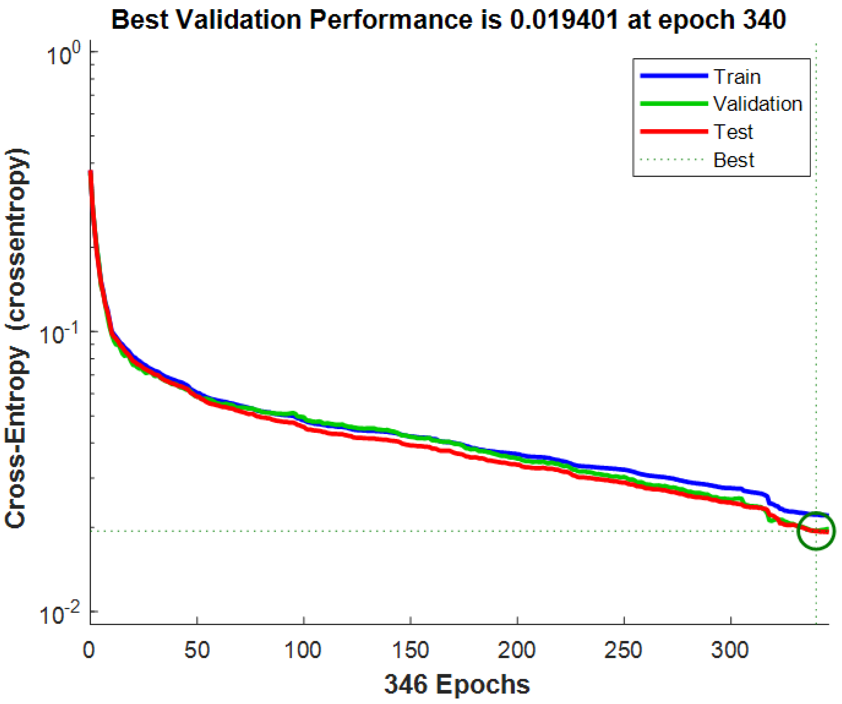
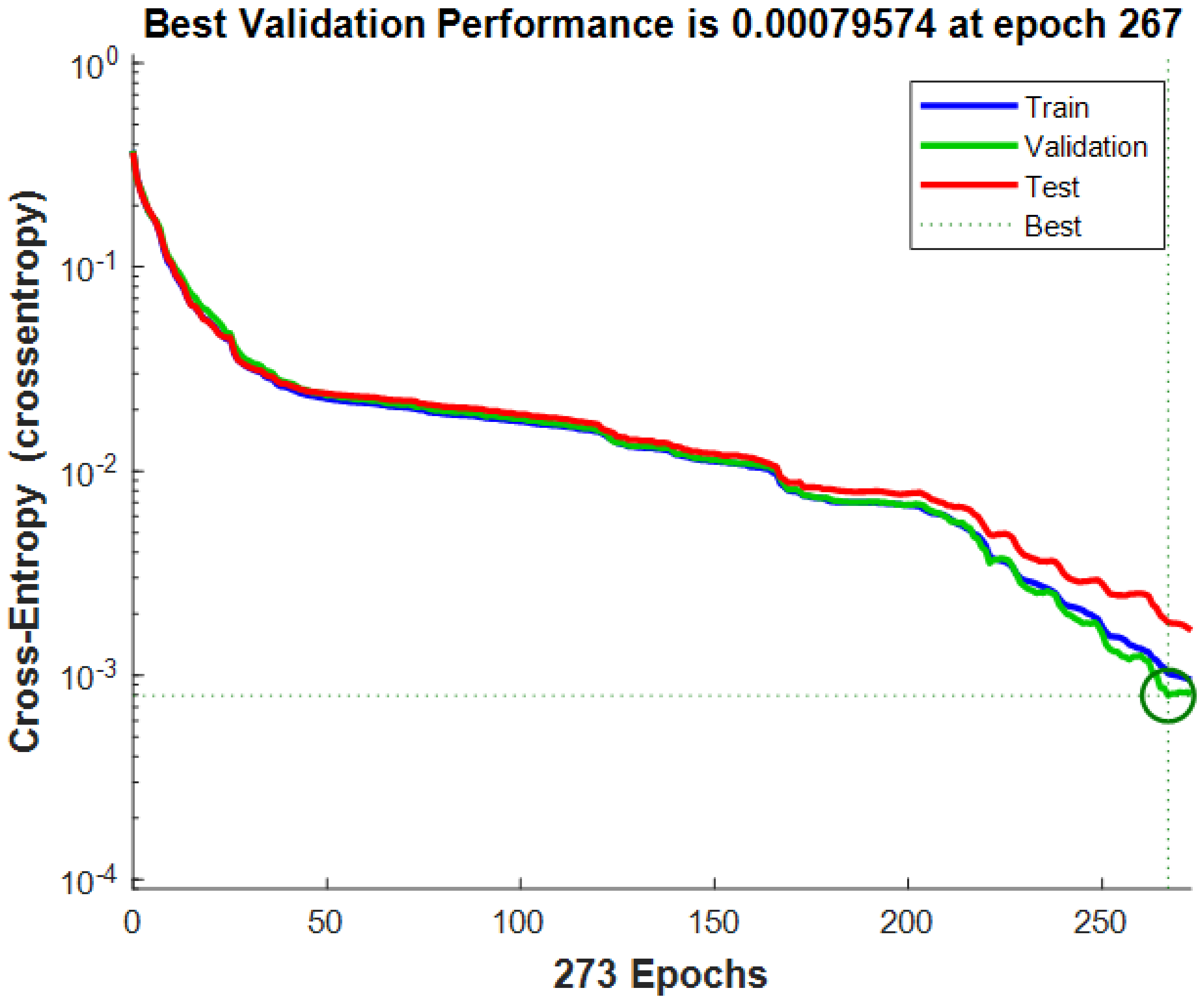
A learning curve is a plot of model learning performance over experience or time. Learning curves are a widely used diagnostic tool in machine learning for algorithms that learn incrementally from a training dataset. Reviewing the learning curves of models during training can be used to diagnose problems with learning, such as an under-fit or over-fit model, as well as whether the training and validation datasets are suitably representative [36]. The following figures (Figure 19, Figure 20 and Figure 21) illustrate the best validation performance plot for the three scenarios.

4. Discussion

The problem was the faults which happened in the DC side of the PV system. As presented in the introduction, the waste of time and effort needed to detect such failures are the greatest struggles in front of the different techniques of detection. So, ascertaining a method depends upon AI techniques that will provide the most suitable solution for that problem. An ANN logarithm was used in this paper to detect and classify those faults. The logarithm model was achieved after passing through several processes as illustrated in the flowcharts in Figure 2 and Figure 7. The results of applying the ANN logarithm for fault detection are discussed here in order to find out the strength and weakness points of the used technique.

The temperature and radiation were monitored for a year, but the data of three days for three hours a day was used in order to simulate the outputs of the PV system as in Table 5. This decision was taken for two reasons. First, as the readings used in the simulation increase, the time of the simulation becomes longer (it may reach the whole day to simulate one type of fault). Second, choosing this time and this date from the year because the date monitored in this period was close to the ideal cases (no disturbance or mistakes in the equipment’s reading).

The idea that the classifier depends on is to differentiate between the P–V and I–V curves of each type of fault. It is known that each P–V or I–V curve can be identified by three main points, which are Pmax, Voc, and Ish as shown in Figure 5 and Figure 6. The P–V and I–V curves of the eight faults are similar but they are not the same.

Table 12. Comparison between the studied faults considering F1 as a reference.

F1 as Reference	Pmax	Voc	Ish
F2	Decrease	Same	Same
F3	Decrease	Decrease	Same
F4	Decrease	Same	Decrease
F5	Decrease	Same	Same
F6	Decrease	Decrease	Same
F7	Decrease	Decrease	Same
F8	Decrease	Decrease	Same

illustrates a comparison between the studied faults considering the no-fault case F1 as a reference.

The PV systems operate all the time during different weather conditions, so dealing with the huge number of P–V and I–V curves makes the ability to differentiate between the faults a difficult task. An ANN logarithm as an AI technique can deal with a huge number of databases. In this paper, the ANN was trained in order to classify the faults that happened in the DC side of the PV systems by considering just the Pmax, Voc, and Ish as inputs to the logarithm (First scenario).

The confusion matrix in Figure 10 confirmed that the logarithm was doing well at classifying most of the faults with good accuracy. For example, if we consider the first scenario, no-fault case F1 was well detected and the ANN logarithm predicted 560 of the inputs data accurately but failed in predicting the other 10 with a 98.2% rate of success. On the other hand, the worst-case scenario happened when the logarithm tried to detect F8. It achieved just 36.3% of success. It predicted 363 of the entered data as hybrid fault F8 but the fact is that they belong to bypass fault F6 and bridge fault F7.

Table 13. Comparison between the three scenarios.

Confusion Matrix Figure 10, Figure 11 and Figure 12	First Scenario	True Detection (Success)	False Detection (Fail)	Success
		560	10	98.2%
		539	39	94.6%
		570	0	100%
		569	1	99.8%
		569	0	100%
		317	254	55.5%
		461	109	80.9%
		207	363	36.3%
		ANN Performance		82.2%
	Second Scenario	565	4	99.3%
		570	0	100%
		570	0	100%
		569	1	99.8%
		568	1	99.8%
		538	33	94.2%
		462	108	81.1%
		477	93	83.7%
		ANN Performance		94.7%
	Third Scenario	570	0	100%
		570	0	100%
		570	0	100%
		570	0	100%
		569	0	100%
		569	2	99.6%
		570	0	100%
		569	1	99.8%
		ANN Performance		99.9%

shows these numbers in detail for the three scenarios. In addition, Figure 11 and Figure 12 shows the confusion matrices for the second and third scenarios.

The error between the predicted value and the actual value gives an indication of logarithm performance and shows how it deals with the entered data. The error histogram of the first scenario in Figure 13 emphasizes the same results that have already been realized using the confusion matrix provided in Figure 10. The error histogram cannot be used to determine where the logarithm failed or succeeded. However, it illustrates that most of the data lie in error equal to 0.04973, whereas the others distributed in errors range from −0.9495 to 0.1494 and from 0.05025 to 0.95. The error histogram gives a good indication of the logarithm performance but it can be enhanced more. The error histogram for the second and the third scenarios are shown in Figure 14 and Figure 15.

The receiver operation curves (ROC) of the first scenario illustrated in Figure 16 are very important to check in order to assess the logarithm performance. They show that the ANN achieves good results in most classes of faults except F6, F7, and F8. These results were achieved by figuring out the area under curves. As the area under the curve becomes bigger, the performance is better. The receiver operation curves for the second and the third scenarios are shown in Figure 17 and Figure 18.

The plot shown in Figure 19 illustrates that the curves decline to reach a point of stability. This point meets a cross-entropy of 0.046638 which achieves the best validating at an epoch number of 130. The dynamic of the three curves shows good fit learning curves also the small gap between the curves emphasizes the same result. The plots for the second and the third scenarios are shown in Figure 20 and Figure 21.

The results of the first scenario were good. The logarithm classifies most of the faults with good accuracy. On the other hand, the logarithm fails in classifying the other faults because those faults have similar characteristics in their P–V and I–V curves as shown in Table 12. So, some modifications and enhancements were added to the first scenario. The modifications were considered in the P–V and I–V curves by adding more points to help the logarithm classify the faults. This operation is explained in Table 11.

Table 14. Comparison between the studied faults taking F1 as a reference.

Figure No.	Assessment Tool	First Scenario	Second Scenario	Third Scenario
10 11 12	Confusion Matrix	83.2%	94.7%	99.9%
13 14 15	Error Histogram Centered at	−0.04973	−0.03745	−0.04996
16 17 18	ROC	Good	Better	Best
19 20 21	Best Validation Performance Plot	0.046698 at epoch 130	0.019401 at epoch 340	0.000079574 at epoch 267

illustrates the difference between the three scenarios in the results.

Considering Table 14 and the provided results, it is obvious that the third scenario achieves the highest level of accuracy in detecting and classifying the faults in the DC side of the PV system because of increasing the number of distinguishing points that are used as inputs to the AI logarithm.

5. Conclusion

Nowadays, the world is dominated by modern technologies and humans can feel their presence all around. AI techniques are one of these technologies which are the backbone of the fourth industrial revolution. The main objective of this paper is to detect and classify the PV faults in the DC side of the PV systems using such AI techniques. The difficulty in finding the fault and classifying its type in a large PV plant can be solved using the proposed technique in this paper. It is found that this solution could make the duty of the PV systems’ maintenance easier, particularly the large-scale ones. Consequently, there is no need to waste time and effort to find the type of fault. In addition, the technique can solve the problem of sudden power reduction because of unexpected failures.

The ANN logarithm, as a subsection of the AI techniques, is applied in order to classify the faults. Three scenarios were created based on a number of parameters used as inputs to the logarithm. These parameters were extracted from the output curves. Matlab and Simulink were the software used to simulate the modeled PV system. Codes were created by Matlab to achieve the purpose of the paper. Several assessment tools (confusion matrixes, ROC curves, Error Histogram, and best validation performance curves) were used to compare between the three scenarios. The third scenario had the best performance of detection and classification with a percentage of 99.9%. The second scenario and first scenario had performance percentages of 94.7% and 83.2%, respectively. Moreover, the Histogram Error, ROC curves, and the best validation curves emphasized the same result. The three scenarios achieved high accuracy depending on real input data. The ANN logarithm can detect faults quickly and with high performance and reliability. The solar PV industry will get benefit from using the proposed technique, especially large-scale PV systems in which this promising solution of fault detection will gain better optimization in terms of time, cost, and efforts of maintenance.

The previous results encourage us to recommend that the power and energy society increase their efforts to involve AI techniques in fault detection and classification. Moreover, investing in AI applications in energy systems could make a huge jump in power production by avoiding any failures. In addition, using AI methods can make the maintenance task easier. The authors recommend giving more attention to data-gathering operations which can accelerate the application of AI methods in power and energy areas. Governmental efforts should also focus on the same purpose. It is recommended to raise the investment in developing different monitoring techniques. These techniques could help in gathering the data with high accuracy and quick processes.

This article achieves its main objective, which is the detection and classification of faults in the DC side of the PV system. However, some enhancements and modifications can make this research perfect. These enhancements will be as follows: generalizing the types of faults in the PV system to include the maximum power tracker faults and the inverter faults. Adding one more objective, which is determining the location of the fault besides the detection and classification will make the AI model purpose general. Validating the proposed AI model in a large-scale PV system using a huge database for training. Using other types of AI techniques like fuzzy, genetic, etc., and then comparing their performance with the ANN logarithm.

References

1. Northcote, J.; Wilson, R. Control and Automation of Distribution Electrical Power Systems, 2rd ed; Taylor & Francis Group: New York, NY, USA, 2019; pp. 154–196. [Google Scholar]
2. Global Cumulative Installed Solar PV Capacity 2019|Statista. Available online: https://www.statista.com/statistics/280220/global-cumulative-installed-solar-pv-capacity (accessed on 5 September 2021).
3. Jia, K.; Gu, C.; Xuan, Z.; Li, L.; Lin, Y. Fault Characteristics Analysis and Line Protection Design Within a Large-Scale Photovoltaic Power Plant. IEEE Trans. Smart Grid 2018, 9, 4099–4108. [Google Scholar] [CrossRef]
4. Firth, S.K.; Lomas, K.J.; Rees, S.J. A simple model of PV system performance and its use in fault detection. Sol. Energy 2010, 84, 624–635. [Google Scholar] [CrossRef] [Green Version]
5. Pradhan, A.; Panda, B. Analysis of Ten External Factors Affecting the Performance of PV System. In Proceedings of the 2017 International Conference on Energy, Communication, Data Analytics and Soft Computing, Chennai, India, 1–2 August 2017. [Google Scholar]
6. Abdulmawjood, K.; Refaat, S.S.; Morsi, W.G. Detection and prediction of faults in photovoltaic arrays: A review. In Proceedings of the 2018 IEEE 12th International Conference on Compatibility, Power Electronics and Power Engineering (CPE-POWERENG 2018), Doha, Qatar, 10–12 April 2018. [Google Scholar]
7. Arani, M.S.; Hejazi, M.A. The comprehensive study of electrical faults in PV arrays. J. Electr. Comput. Eng. 2016, 2016, 8712960. [Google Scholar]
8. Sulas-Kern, D.B.; Johnston, S.; Wang, M.H. Monitoring, Diagnosis, and Power Forecasting for Photovoltaic Fields: A Review. Int. J. Photoenergy 2017, 2017, 2008–2012. [Google Scholar]
9. Chao, K.H.; Ho, S.H.; Meydbray, J. Modeling and fault diagnosis of a photovoltaic system. Electr. Power Syst. Res. 2008, 78, 97–105. [Google Scholar] [CrossRef]
10. Gokmen, N.; Karatepe, E.; Silvestre, B.; Celik, B.; Ortega, P. An efficient fault diagnosis method for PV systems based on operating voltage-window. Energy Convers. Manag. 2013, 73, 350–360. [Google Scholar] [CrossRef]
11. Braun, H.; Buddha, S.T.; Krishnan, V.; Spanias, A.; Tepedelenlioglu, C.; Yeider, T.; Takehara, T. Signal processing for fault detection in photovoltaic arrays. In Proceedings of the 2012 IEEE International Conference on Acoustics, Speech and Signal Processing (ICASSP), Kyoto, Japan, 25–30 March 2017. [Google Scholar]
12. Xu, X.; Wang, H.; Zuo, H. Method for diagnosing photovoltaic array fault in solar photovoltaic system. In Proceedings of the 2011 Asia-Pacific Power and Energy Engineering Conference, Wuhan, China, 25–28 March 2011. [Google Scholar]
13. Huang, Z.; Guo, L. Research and implementation of microcomputer online fault detection of solar array. In Proceedings of the 2009 4th International Conference on Computer Science & Education, Nanning, China, 25–28 July 2009. [Google Scholar]
14. Zhao, Y.; Lehman, B.; Ball, R.; Mosesian, J.; De Palma, J.F. Outlier detection rules for fault detection in solar photovoltaic arrays. In Proceedings of the 2013 Twenty-Eighth Annual IEEE Applied Power Electronics Conference and Exposition (APEC), Long Beach, CA, USA, 17–21 March 2013. [Google Scholar]
15. Houssein, A.; Heraud, N.; Souleiman, I.; Pellet, G. Monitoring and fault diagnosis of photovoltaic panels. In Proceedings of the 2010 IEEE International Energy Conference, Manama, Bahrain, 18–21 December 2010. [Google Scholar]
16. Solórzano, J.; Egido, M.A.; Rees, S.J. Automatic fault diagnosis in PV systems with distributed MPPT. Energy Convers. Manag. 2013, 76, 925–934. [Google Scholar] [CrossRef]
17. Drews, A.; De Keizer, A.C.; Beyer, H.G.; Lorenz, E.; Betcke, J.; van Sark, W.G.J.H.M.; Heydenreich, W.; Wiemken, E.; Stettler, S. Monitoring and remote failure detection of grid-connected PV systems based on satellite observations. Sol. Energy 2007, 81, 548–564. [Google Scholar] [CrossRef] [Green Version]
18. Chen, Z.; Wu, L.; Cheng, P.; Lin, P.; Wu, Y.; Lin, W. Intelligent fault diagnosis of photovoltaic arrays based on optimized kernel extreme learning machine and I-V characteristics. Appl. Energy 2017, 204, 912–931. [Google Scholar] [CrossRef]
19. Dhimish, M.; Holmes, V.; Mehrdadi, B.; Dales, M.; Mather, P. Photovoltaic fault detection algorithm based on theoretical curves modelling and fuzzy classification system. Energy 2017, 140, 276–290. [Google Scholar] [CrossRef]
20. Hutchison, D. Advanced in swarm intelligence. In Proceedings of the International Conference on Swarm Intelligence (ACSI), Beijing, China, 12–15 June 2010. [Google Scholar]
21. Cheng, Z.; Zhong, D.; Li, B.; Liu, Y. Research on fault detection of PV array based on data fusion and fuzzy mathematics. In Proceedings of the 2011 Asia-Pacific Power and Energy Engineering Conference, Wuhan, China, 25–28 March 2011. [Google Scholar]
22. Ducange, P.; Fazzolari, M.; Lazzerini, B.; Marcelloni, F. An intelligent system for detecting faults in photovoltaic fields. In Proceedings of the 2011 11th International Conference on Intelligent Systems Design and Applications, Córdoba, Spain, 22–24 November 2011. [Google Scholar]
23. Coleman, A.; Zalewski, J. Intelligent Fault Detection and Diagnostics. In Proceedings of the The 6th IEEE International Conference on Intelligent Data Acquisition and Advanced Computing Systems: Technology and Applications, Prague, Czech Republic, 15–17 September 2011. [Google Scholar]
24. Syafaruddin; Karatepe, E.; Hiyama, T. Controlling of artificial neural network for fault diagnosis of photovoltaic array. In Proceedings of the 2011 16th International Conference on Intelligent System Applications to Power Systems, Hersonisso, Greece, 25 September 2011. [Google Scholar]
25. Zhao, Y.; Yang, L.; Lehman, B.; De Palma, J.F.; Mosesian, J.; Lyons, R. Decision tree-based fault detection and classification in solar photovoltaic arrays. In Proceedings of the 2012 Twenty-Seventh Annual IEEE Applied Power Electronics Conference and Exposition (APEC), Orlando, FL, USA, 5–9 February 2012. [Google Scholar]
26. Zhao, Y.; Lehman, B.; Ball, R.; De Palma, J.F. Graph-based semi-supervised learning for fault detection and classification in solar photovoltaic arrays. ECCE 2013, 30, 1628–1634. [Google Scholar]
27. Hu, Y.; Gao, B.; Song, X.; Tian, G.Y.; Li, K.; He, X. Photovoltaic fault detection using a parameter based model. Sol. Energy 2013, 96, 96–102. [Google Scholar] [CrossRef]
28. Vergura, S.; Acciani, G.; Otani, K.; Kato, K.; Ishida, M. A finite-element approach to analyze the thermal effect of defects on silicon-based PV cells. IEEE Trans. Ind. Electron. 2012, 59, 3860–3867. [Google Scholar] [CrossRef]
29. Takashima, T.; Yamaguchi, J.; Otani, K.; Kato, K.; Ishida, M. Experimental studies of failure detection methods in PV module strings. In Proceedings of the IEEE 4th World Conference on Photovoltaic Energy Conversion, Waikoloa, HI, USA, 7–12 May 2006. [Google Scholar]
30. Takashima, T.; Yamaguchi, J.; Ishida, M. Fault detection by signal response in PV module strings. In Proceedings of the 2008 33rd IEEE Photovoltaic Specialists Conference, San Diego, CA, USA, 11–16 May 2006. [Google Scholar]
31. Nguyen, X.H. Matlab/Simulink Based Modeling to Study Effect of Partial Shadow on Solar Photovoltaic Array. Environ. Syst. Res. 2015, 4, 20. [Google Scholar] [CrossRef]
32. Mahto, R.V.; Sharma, D.K.; Xavier, D.X.; Raghavan, R.N. Improving performance of photovoltaic panel by configurability in partial shading condition. Photonics Energy 2020, 10, 042004. [Google Scholar]
33. Understanding Confusion Matrix|by Sarang Narkhede|Towards Data Science. Available online: https://towardsdatascience.com/understanding-confusion-matrix-a9ad42dcfd62 (accessed on 19 February 2022).
34. What is the error histogram in neural network matlab? Available online: https://www.mathworks.com/matlabcentral/answers/495218-what-is-the-error-histogram-in-neural-network-matlab (accessed on 19 February 2022).
35. Understanding AUC—ROC Curve|by Sarang Narkhede|Towards Data Science. Available online: https://towardsdatascience.com/understanding-auc-roc-curve-68b2303cc9c5 (accessed on 19 February 2022).
36. How to use Learning Curves to Diagnose Machine Learning Model Performance. Available online: https://machinelearningmastery.com/learning-curves-for-diagnosing-machine-learning-model-performance/ (accessed on 27 February 2022).
Figure 1. Fault detection methods.
Sustainability 14 13815 g001
Figure 2. The flowchart of process progression.
Sustainability 14 13815 g002
Figure 3. Single solar module configuration under normal operation conditions (NOC).
Sustainability 14 13815 g003
Figure 4. The PV system configuration.
Sustainability 14 13815 g004
Figure 5. The P–V curve of the PV system under NOC.
Sustainability 14 13815 g005
Figure 6. The I–V curve of the PV system under NOC.
Sustainability 14 13815 g006
Figure 7. The ANN logarithm configuration.
Sustainability 14 13815 g007
Figure 8. The ANN configuration for fault detection in the PV system.
Sustainability 14 13815 g008
Figure 9. Confusion Matrix for two classes’ classification.
Sustainability 14 13815 g009
Figure 10. The confusion matrices for the first scenario. (a) Training confusion matrix; (b) Validating confusion matrix; (c) Test confusion matrix; and (d) All confusion matrix.
Sustainability 14 13815 g010
Figure 11. This is the confusion matrices for the second scenario. (a) Training confusion matrix; (b) Validating confusion matrix; (c) Test confusion matrix; and (d) All confusion matrix.
Sustainability 14 13815 g011
Figure 12. These are the confusion matrices for the third scenario. (a) Training confusion matrix; (b) Validating confusion matrix; (c) Test confusion matrix; and (d) All confusion matrix.
Sustainability 14 13815 g012
Figure 13. The error histogram for the first scenario.
Sustainability 14 13815 g013
Figure 14. The error histogram for the second scenario.
Sustainability 14 13815 g014
Figure 15. The error histogram for the third scenario.
Sustainability 14 13815 g015
Figure 16. These are the Receiver Operating Characteristic curves for the first scenario. (a) Training ROC; (b) Validating ROC; (c) Test ROC; and (d) All ROC.
Sustainability 14 13815 g016
Figure 17. These are the Receiver Operating Characteristic curves for the second scenario. (a) Training ROC; (b) Validating ROC; (c) Test ROC; and (d) All ROC.
Sustainability 14 13815 g017
Figure 18. These are the Receiver Operating Characteristic curves for the third scenario. (a) Training ROC; (b) Validating ROC; (c) Test ROC; and (d) All ROC.
Sustainability 14 13815 g018aSustainability 14 13815 g018b
Figure 19. Best Validation Performance for the first scenario.
Sustainability 14 13815 g019
Figure 20. Best Validation Performance for the second scenario.
Sustainability 14 13815 g020
Figure 21. Best Validation Performance for the third scenario.
Sustainability 14 13815 g021