Trade Credit Insurance for the Capital-Constrained Supplier

Abstract

This paper examines the role of trade credit insurance in a supply chain consisting of a capital-constrained supplier and a capital-constrained retailer. The retailer faces stochastic market demand and seeks trade credit from the supplier. The supplier, who is the Stackelberg game leader, decides the production quantity and the insurance coverage rate. We find that when the supplier’s initial capital is not sufficient, the use of trade credit insurance may reduce the trade quantity and the expected profit of the retailer. However, when the initial capital of the supplier is sufficient, the use of trade credit insurance will always increase the trade quantity. In the extension, we assume the supplier will face a potential financing cost if the net income is lower than the threshold. We find that if the insurance company has to keep its expected return positive and has no way to invest the insurance premium, the supplier will never buy the trade credit insurance no matter how much the marginal financing cost is when threshold is outside a certain range. Both the results and the methods in this paper can help businesses achieve a balance of funds and the logistics of the supply chain and risks, thereby improving the effectiveness of the supply chain operation.

1. Introduction

Trade credit is a short-term financing agreement between suppliers and retailers that allows retailers to delay payments after receiving commodities or services. According to a report from the World Trade Organization (WTO) [1], up to 80 percent of global trade involves trade financing approaches, and the market for trade finance has reached USD 12 trillion per year. It has been shown that trade credit can greatly facilitate trade [2,3,4,5]. However, a supplier that offers trade credit may face some risks. First, if the actual market demand is not high enough, the retailer may not obtain enough money to pay the supplier and may default. Moreover, a change in policy or the outbreak of health epidemics can have a catastrophic impact on trade [6], and the retailer may default. When the retailer defaults, the supplier may not only lose the payback from the retailer, it may also need to finance itself and thus may face a financing cost. In the worst case, the supplier will go bankrupt itself. For example, in China, in order to quickly seize a market opportunity at an early stage, many ‘new retail’ enterprises recruited a large number of franchised retailers. The retailers only paid money to rent and decorate the stores and to hire employees. They usually did not have a large amount of working capital. The enterprises provided them with goods but did not charge them immediately. They were to pay the supplier after they completed the sales. However, due to fierce market competition and the epidemic, a large number of retail stores failed to meet expectations, resulting in the default of payment for goods, and enterprises fell into crisis.

In order to avoid the non-payment risk, the supplier can purchase trade credit insurance (also known as credit insurance, business credit insurance, or export credit insurance), which insures manufacturers, traders, and providers of services against the risk that their buyers will not pay (after bankruptcy or insolvency) or pay very late. This popular form of protection can not only help the supplier reduce credit risk-related losses, it also can help the supplier obtain better financing terms from banks, some of which now require firms to purchase trade credit insurance before providing money [7].

According to the International Credit Insurance and Surety Association, in 2020, the trade credit insurance exposure of its members was close to EUR 2.5 trillion, and the insurance premium was close to EUR 6.5 billion. The trade credit insurance policy will pay out a portion of the outstanding debt. This percentage usually ranges from 75% to 95% of the invoice amount but may be higher or lower depending on the type of coverage that was purchased. In this paper, we assume the trade credit insurance coverage rate ranges from 0% (does not use trade credit insurance) to 100% of the total credit that the supplier offers to the retailer.

Although a number of studies have shown the expansionary effect of trade credit insurance or guarantees on trade [8,9,10], to the best of our knowledge, few scholars have explored how a capital-constrained supplier should distribute its capital between trade credit and trade credit insurance. However, we believe that this situation is common in practice and thus is worth studying. We show that for a capital-constrained supplier, even if it will face a potential cost when it cannot obtain payment, it may decide not to use trade credit insurance at all. In addition, when the initial capital of the supplier is not sufficient, the use of trade credit insurance will reduce the production quantity. This finding is very different from the previous ones.

The remainder of the paper is organized as follows. We review the related literature in the next section. We introduce the model in Section 3. Then, in Section 4, we investigate the strategies for the retailer and the supplier. We extend the model to investigate the case where the supplier faces a potential financing cost. We conclude the study in Section 6.

2. Literature Review

This work is related to two streams of literature: trade credit insurance and supply chain management.

In terms of the trade credit insurance literature, most articles have focused on the effect of insurance on trade, the financing terms, and asymmetric information. For instance, Funatsu [8] assumed that the insurance premium rate was fixed and studied the impact of trade credit insurance on an exporter’s output decisions. He determined that with the use of trade credit insurance, the supplier produced more products. Ford et al. [9] extended Funatsu’s research by permitting the premium rate to vary with the size of the insurance coverage taken. Rienstra–Munnicha and Turvey [10] used the empirical results to prove the expansionary effect of insurance on trade. Li et al. [7] extended the models of Funatsu [8] and Ford et al. [9] to explore the operation management of the firm and the risk control of the bank. Even though they all considered the default risk due to the market risk and political risk, instead of linking the default probability to the market demand distribution, they just assumed a payment loss rate $\alpha$ distributed between zero and one to deal with all kinds of risks. Li et al. [11] studied the case in which there was one well-capitalized supplier and one capital-constrained retailer. They used stochastic demand to investigate the equilibrium wholesale price, the equilibrium order quantity, the equilibrium insurance coverage, and the equilibrium insurance premium. Our model is similar to their model except that we consider a capital-constrained supplier and a capital-constrained retailer. Yang et al. [12] identified the smoothing role and the monitoring role of trade credit insurance; they also investigated the cancelable term and found that noncancelable contracts were relatively more attractive when the acquired information was verifiable. They contributed to the terms design of the trade credit contract, while we focus on the allocation of the limited capital. In their model, they assumed the buyer had a fixed need, and there were three levels of default probabilities, while we use the stochastic demand to investigate the default conditions. However, we also share some assumptions. They assumed that the supplier may face a financing cost if it cannot receive enough money, and we apply a similar idea to our model. Li et al. [13] investigated the insuring strategy of the retailer and the manufacturer in a capital-constrained supply chain. In their model, the supplier was not capital constrained, and the supplier and the retailer had to buy the 100% coverage trade credit insurance jointly. They showed that the adoption of trade credit insurance improved the order quantity of the retailer, the performance of each supply chain participant, and supply chain efficiency, all of which has been shown in many other papers. However, since we consider the supplier to have limited initial capital, and partial coverage insurance is available, we prove that this conclusion is not always true.

In terms of the supply chain management literature, many people have studied capital-constrained players and different financial tools. For buyer-led finance, the most common financial forms include advance selling [14,15,16,17,18,19], buyer intermediation financing [20], and reverse factoring [21,22]. Deng et al. [19] considered a supply chain with multiple suppliers and one retailer. They characterized the impact of the initial capital, production cost, and other features on the optimal financing schemes and derived equilibrium solutions for both financing methods. Kouveils and Xu [22] exhaustively analyzed factoring and reverse-factoring financing offered by a retailer and a bank loan from a competitive bank industry and identified the optimal financing scheme under different situations by comparing the equilibrium of each financing scheme. The work also provided a detailed review of factoring financing. This paper, on the other hand, is mostly related to the supplier-led supply chain with the supplier offering trade credit. This type of financial structure is more common in practice and theory [23,24,25,26,27,28,29,30,31,32,33,34]. Xu and Birge [23] examined a channel consisting of one supplier and one capital-constrained retailer, where the retailer could obtain credit either from a competitive bank market or from the supplier. They were among the first group of people to discuss the relationship between a firm’s inventory decisions and its capital constraints and capital structure. Li and Gu [31] formulated a time-continuous model with constant demand and studied the operating decisions and accounts-receivable factoring financial scheme. Kouvelis and Zhao [25] considered a newsvendor-like retailer with stochastic demand and concluded that trade credit contracts do improve the supply chain efficiency but are not a coordinating contract. Chen [27] found that trade credit better integrated the supply chain than bank credit by centralizing the financing of distribution at the manufacturer. He further compared bank versus trade credit under a classical supply chain contract and a revenue sharing contract. Shi et al. [32] explored how bankruptcy cost affected a retailer’s financing mode selection decision between bank credit financing and trade credit financing. Mahato et al. [33] examined the case where a supplier offered order-quantity-dependent partial trade credit to a retailer. Wang et al. [34] established a supply chain comprising one supplier and two capital-constrained retailers to investigate the supplier’s and retailers’ preferences for different trade credit provision patterns. The emerging new-type financing platforms including e-commerce platforms [35,36], peer-to-peer platforms [37], etc., have also been widely studied. This paper is related to this supply chain management literature, because we also include similar settings and game processes (Stackelberg game) in our model to investigate the relationship between the wholesale price, order quantity, and coverage rate.

To summarize, the differences between this paper and the abovementioned literature are mainly as follows. This paper investigates the case when the supplier faces capital constraints and aims to find out how the supplier should distribute its money, or specifically, how much money it should use to produce the products and how much money it should use to buy the credit insurance. This paper also investigates the equilibrium wholesale price and the equilibrium quantity.

3. Model Setup

We considered a supply chain with one capital-constrained supplier (he) and one capital constrained retailer (she). We assumed that the supplier was the Stackelberg leader in the game, and he could decide the wholesale price and how much credit to offer the retailer. The supplier could also decide whether to buy the trade credit insurance. The sequence of events was as follows:

At time 0, the supplier determined the wholesale price w for the retailer. We assumed $c\le w\le 1$. After knowing the wholesale price, the retailer immediately informed the supplier about their demand for the commodity, $q_r$, and financing request. The supplier decided how much credit to offer the retailer. In other words, the supplier decided the quantity to produce, $q^{*}$, and $q^{*}\le q_r$. Here, we assumed that the supplier would use all the available capital to satisfy the retailer’s request first. In addition, the supplier also decided whether to purchase trade credit insurance with an insurance coverage rate of $\theta$ at a premium rate s.

At time 1, the retailer needed to repay the money she owed to the supplier or the total revenue she received. Here, we assume the salvage commodities had no value, and the retail price was 1. Afterward, if the supplier bought trade credit insurance, the insurance company compensated the loss to the supplier. Similar to the other supply chain literature [38], we assumed the ex ante demand distribution function was $F\left(x\right)$ and had the following properties: (i) $F\left(x\right)$ is absolutely continuous with density $f\left(x\right)>0$ on (0, ∞), (ii) $F\left(x\right)$ has a finite mean, and (iii) its hazard rate $h\left(x\right)=f\left(x\right)/(1-F(x\left)\right)$ is increasing in x. Let $H\left(x\right)=xh\left(x\right)$ denote the generalized failure rate. Then, $H\left(x\right)$ is monotonically increasing in x. We also assumed that the supplier and the retailer only participated in the trade when their expected returns were positive.

The notations are summarized in

Table 1. Notations.

Notation	Description
c	marginal cost
q	delivered quantity
${-}^{*}$	the equilibrium solution of a variable
w	wholesale price for the retailer
$\theta$	insurance coverage rate
s	insurance premium rate
D	random market demand
$F\left(x\right)$ and $f\left(x\right)$	CDF and PDF of D
${\pi }_r$	expected profit of the retailer
${\pi }_s$	expected profit of the supplier
T	capital threshold
l	marginal financing cost
K	capital constraint of the supplier
$K_r$	capital constraint of the retailer

:

4. Equilibrium for the Supply Chain

For a retailer with initial capital $K_r$, she can postpone part of her payment, ${(wq-K_r)}^{+}$, to the supplier at first (${\left(X\right)}^{+}=max\{X,0\}$). When the payment is due, her profit will be the difference between the revenue she received, $min\{D,q\}$, and the amount she needs to pay the supplier, $wq$. However, if the retailer does not receive enough revenue to cover the liability, she will pay back all the money she received and make zero profit. Thus, the retailer’s expected profit can be written in the following way:

$$\begin{array}{cc}\hfill {\pi }_r& =\mathbb{E}\left(max\{min\{D,q\}-wq,-K_r\}\right)\hfill \\ \hfill & =\left\{\begin{array}{c}{\int }_0^{wq-K_r}(-K_r)dF+{\int }_{wq-K_r}^q(x-wq)dF+{\int }_q^{\infty }(q-wq)dF(K_r<wq)\hfill \\ {\int }_0^q(x-wq)dF+{\int }_q^{\infty }(q-wq)dF(K_r\ge wq)\hfill \end{array}\right.\hfill \end{array}$$

(1)

The supplier’s objective is to maximize his expected profit. If the supplier does not use trade credit insurance, his expected profit is equal to the payment from the retailer minus the manufacturing cost:

$$\begin{array}{cc}\hfill {\pi }_s& =\left\{\begin{array}{c}\mathbb{E}(min\{D,wq-K_r\}+K_r-cq)(K_r<wq)\hfill \\ (w-c)q(K_r\ge wq)\hfill \end{array}\right.\hfill \\ \hfill & =\left\{\begin{array}{c}{\int }_0^{wq-K_r}xdF+{\int }_{wq-K_r}^{\infty }(wq-K_r)dF+K_r-cq(K_r<wq)\hfill \\ (w-c)q(K_r\ge wq)\hfill \end{array}\right.\hfill \end{array}$$

(2)

If the retailer asks for trade credit, and the supplier buys trade credit insurance, the insurance company will ensure that the supplier receives at least $\theta (wq-K_r)$ at the end of the season. His expected profit now equals the payment from the retailer plus the claim payment minus the manufacturing cost and the outgoing insurance premium:

$$\begin{array}{cc}\hfill {\pi }_s^{in}& =\mathbb{E}(max\{min\{D,w^{in}{q}^{in}-K_r\},\theta (w^{in}{q}^{in}-K_r)\}+K_r-c{q}^{in}-\theta s(w^{in}{q}^{in}-K_r))\hfill \\ \hfill & ={\int }_0^{\theta (w^{in}{q}^{in}-K_r)}\theta (w^{in}{q}^{in}-K_r)dF+{\int }_{\theta (w^{in}{q}^{in}-K_r)}^{(w^{in}{q}^{in}-K_r)}xdF+{\int }_{(w^{in}{q}^{in}-K_r)}^{\infty }(w^{in}{q}^{in}-K_r)dF\hfill \\ \hfill & +K_r-c{q}^{in}-\theta s(w^{in}{q}^{in}-K_r)(K_r<w^{in}{q}^{in})\hfill \end{array}$$

(3)

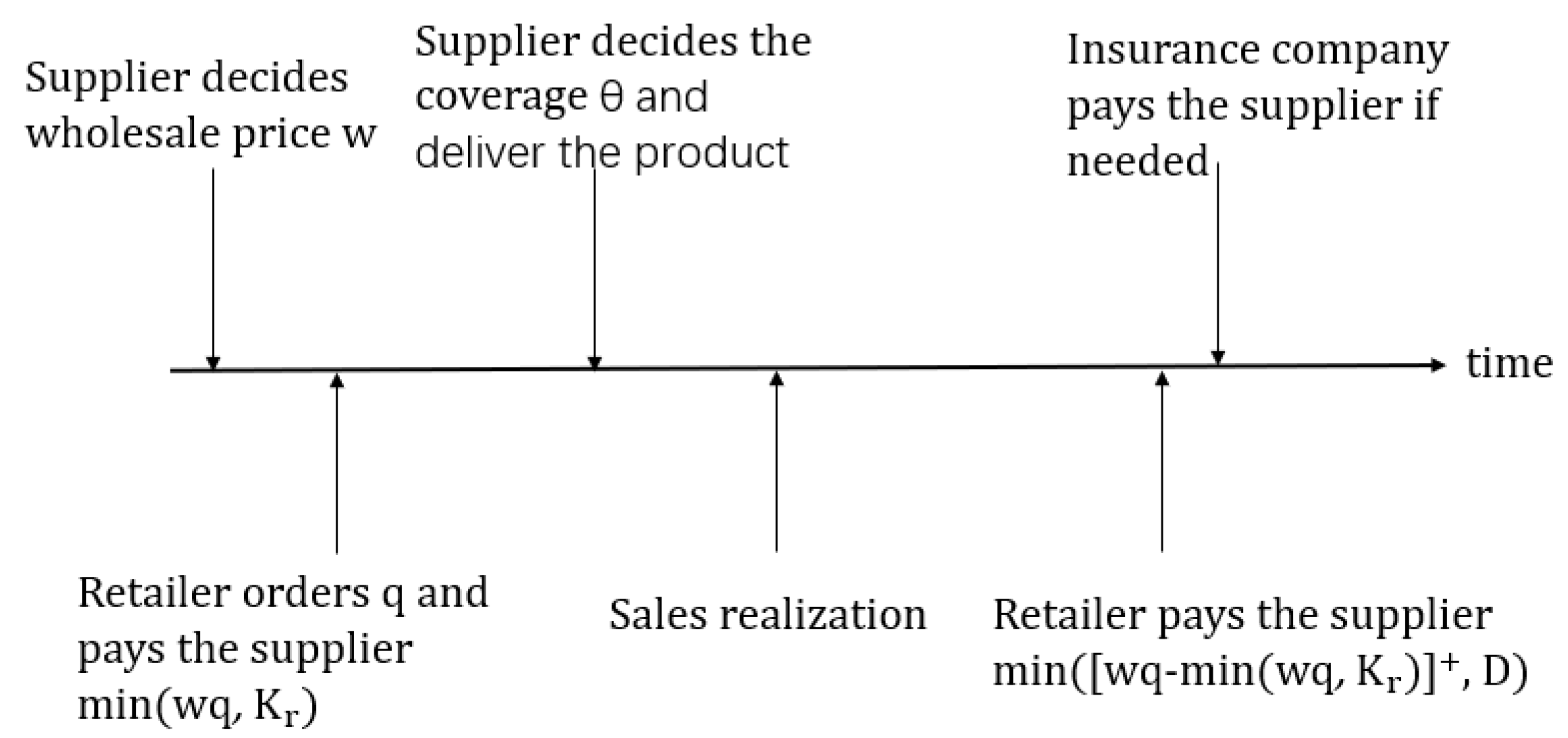
The sequence of events is shown in Figure 1.

After the supplier decides the wholesale price, the retailer decides the quantity of the product to order from the supplier to maximize her profit: $\stackrel{max}{q}{\pi }_r$.

Proposition 1. 

(1) When the wholesale price is given, the quantity of the product that the retailer wants to order, $q_r$, is unique. (2) $\frac{\mathrm{d}{q}_r}{\mathrm{d}w}<0$.

The proof of Proposition 1 is in Appendix A.

Corollary 1. 

When $H\left(q_r\right)>1$, $\frac{\mathrm{d}\left(w{q}_r\right)}{\mathrm{d}w}>0$, and when $H\left(q_r\right)<1$, $\frac{\mathrm{d}\left(w{q}_r\right)}{\mathrm{d}w}<0$.

From Proposition 1, we see that with the increase in the wholesale price, the optimal quantity for the retailer decreases. So, if the target of the supplier is to maximize the sales quantity, he should offer a low wholesale price. From Corollary 1, we see that when the marginal cost is so low that $1-H\left(q_r\left(c\right)\right)<0$, with the increase in the wholesale price, the total revenue that the supplier can obtain first increases, and after the wholesale price becomes higher than the threshold $w_0$, the revenue decreases. If the supplier wants high revenue in a certain season, setting the wholesale price as $w_0$ may be a good idea.

Since the supplier is the Stackelberg leader, he knows how the retailer will react. He will determine the wholesale price w to maximize his expected profit. The upper bound of the total amount of capital that can be used to produce the products is $K+K_r$, if we assume that the optimal wholesale price for the supplier without a capital constraint is $w_s$, since $\frac{\mathrm{d}{q}_r}{\mathrm{d}w}<0$, then when $c{q}_r<K+K_r$, $w^{*}=w_s$, and when $c{q}_r=K+K_r$, $w^{*}\ge w_s$.

Proposition 2. 

The equilibrium wholesale price $w^{*}$ is unique.

The proof of Proposition 2 is in Appendix A.

To summarize, when the supplier does not use trade credit insurance, we obtain the following system:

$$\begin{array}{cc}\hfill \underset{q}{max}& {\pi }_r\hfill \end{array}$$

(4)

$$\begin{array}{cc}\hfill \underset{w}{max}& {\pi }_s\hfill \end{array}$$

(5)

$$\begin{array}{cc}\hfill s.t.cq& \le K+K_r\hfill \end{array}$$

(6)

$$\begin{array}{cc}\hfill {\pi }_r& \ge 0\hfill \end{array}$$

(7)

$$\begin{array}{cc}\hfill {\pi }_s& \ge 0\hfill \end{array}$$

(8)

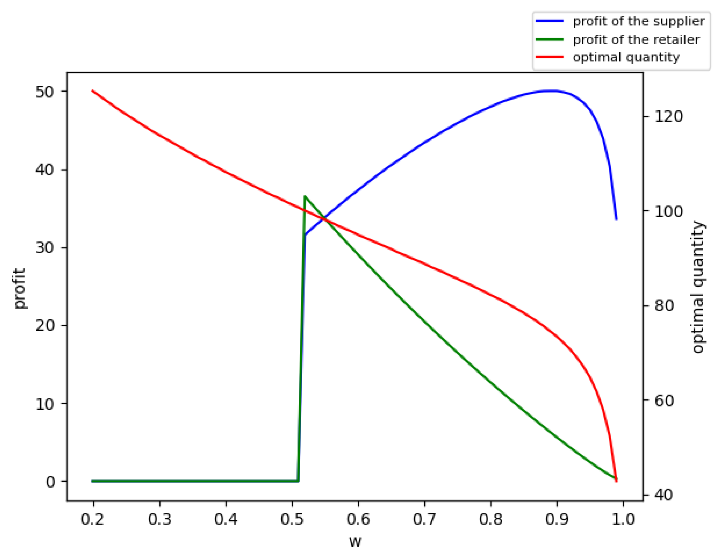
We illustrate these results in Figure 2; referring to the previous research [39], we assumed the market demand D∼$N(100,30)$ (normal distribution with mean = 100 and standard deviation = 30), with $c=0.2$ and $K_r=5$.

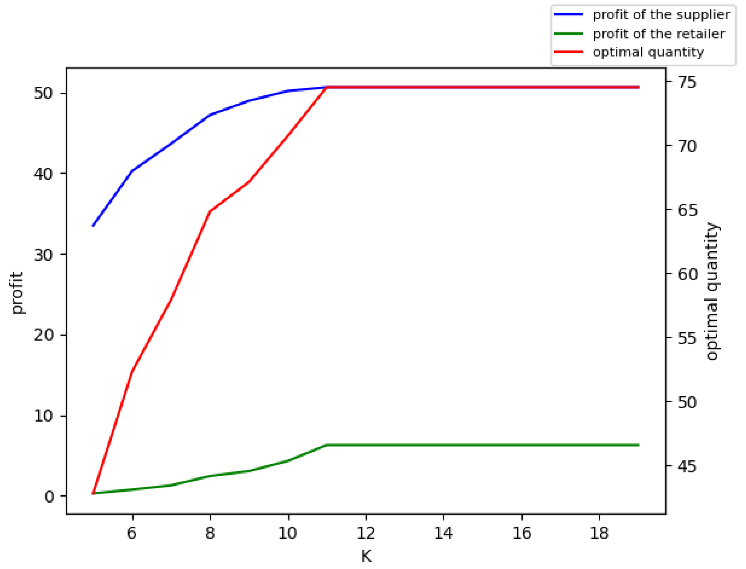
The equilibrium solution was $w^{*}=0.89\left(0.8899\right)$, $q^{*}=75\left(74.5\right)$, ${\pi }_r=6.29$, and ${\pi }_s=50$. We retained two decimal places for the profits and the wholesale price.

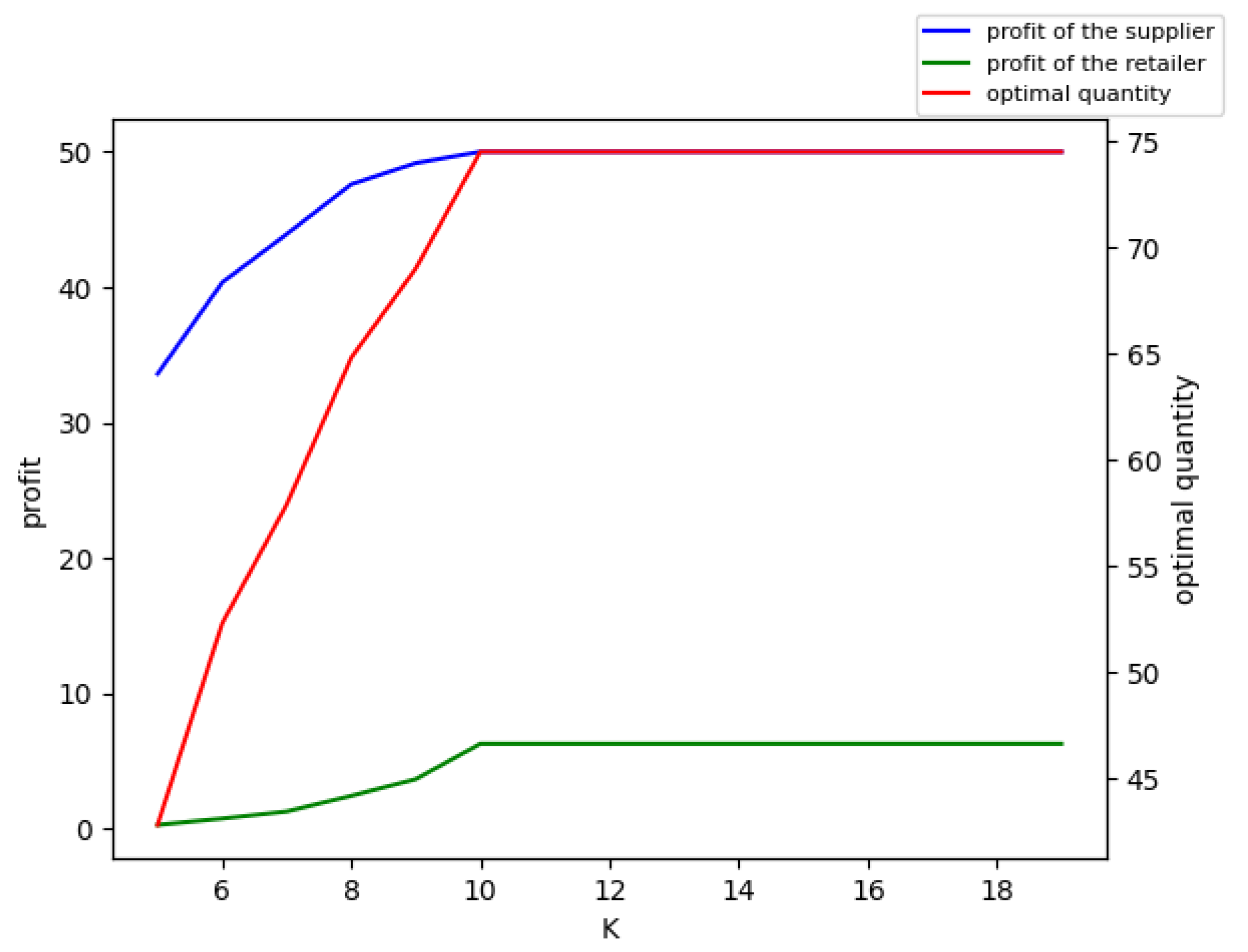
From Figure 3, we can see that before reaching their maximum values, the profit of the supplier, the profit of the retailer, and the optimal quantity all increased with the increase in the initial capital of the supplier.

When $w^{in}{q}^{in}\ge K_r$, $K+K_r-c{q}_r^{in}>0$, and the supplier uses trade credit insurance, the insurance decision of the supplier does not affect the retailer’s expected profit function and her order decision (the relationship between the order quantity and the wholesale price) directly, but it may affect the retailer through the wholesale price. The equilibrium wholesale price $w^{in*}$ satisfies the first-order condition $\frac{\mathrm{d}{\pi }_s^{in}}{\mathrm{d}{w}^{in}}=0$ or $w^{in*}\to 1$. The supplier also has to decide the proportion of the upcoming payment from the retailer to be secured. Since we assume that the supplier has to satisfy the retailer’s request first, then the capital left that can be used to purchase insurance is $K+K_r-c{q}_r^{in}$. For a risk neutral supplier, he has to make sure that ${\pi }_s^{in}\ge {\pi }_s$, or he will not use trade credit insurance.

If we assume that $w^{in}$ and $q^{in}$ are given, then the supplier will use the trade credit only when

$$\theta s(w^{in}{q}^{in}-K_r)\le {\int }_0^{\theta (w^{in}{q}^{in}-K_r)}(\theta (w^{in}{q}^{in}-K_r)-x)dF$$

(9)

It is easy to see that with the increase in $\theta$, the upper bound of s decreases. In other words, when the insurance premium is not low enough, the supplier can only choose a high coverage rate or not to use trade credit insurance at all.

Lemma 1. 

For a risk neutral supplier, when the insurance premium s is given, the equilibrium ${\theta }^{*}\ge \underline{\theta }$ or ${\theta }^{*}=0$, where $\underline{\theta }$ solves $\underline{\theta }s(wq-K_r)={\int }_0^{\underline{\theta }(wq-K_r)}(\underline{\theta }(wq-K_r)-x)dF$.

When $w^{in}$ and $q^{in}$ are given and the initial capital is sufficient, we have

$$\frac{\mathrm{d}{\pi }_s^{in}}{\mathrm{d}\theta }=(w^{in}{q}^{in}-K_r)[F\left(\theta (w^{in}{q}^{in}-K_r)\right)-s].$$

(10)

We can see that if $F^{-1}\left(s\right)<w^{in}{q}^{in}-K_r$, when $\theta$ is less than $\frac{F^{-1}\left(s\right)}{w^{in}{q}^{in}-K_r}$, ${\pi }_s^{in}$ decreases with the increase in $\theta$, and ${\pi }_s^{in}$ obtains its minimum when $\theta =\frac{F^{-1}\left(s\right)}{w^{in}{q}^{in}-K_r}$. So, we obtain the following proposition.

Proposition 3. 

When $w^{in}$ and $q^{in}$ are given, $w^{in}{q}^{in}\ge K_r$ and $K+K_r\ge c{q}^{in}$,

$$\begin{array}{cc}\hfill {\theta }^{*}& =\left\{\begin{array}{c}1\left(s\le {\int }_0^{(w^{in}{q}^{in}-K_r)}(1-\frac{x}{w^{in}{q}^{in}-K_r})dF\mathrm{and}CL\ge 1\right)\hfill \\ CL\left(s\le {\int }_0^{\left(\frac{K+K_r-c{q}^{in}}{s}\right)}(1-\frac{sx}{K+K_r-c{q}^{in}})dF\mathrm{and}CL<1\right)\hfill \\ 0\left(otherwise\right)\hfill \end{array}\right.\hfill \end{array}$$

(11)

where $CL$=$\frac{K+K_r-c{q}^{in}}{s(w^{in}{q}^{in}-K_r)}$.

From Proposition 3, we can see that when $w^{in}$ and $q^{in}$ are given, if there is enough money left after taking into account the production cost, when the insurance premium is lower than the threshold, the supplier will buy total coverage insurance; however, if there is not enough money left, the threshold becomes lower with the decrease in the money left, and the supplier will use all the money to buy the insurance when the insurance premium is lower than the threshold.

To summarize, if the supplier can use trade credit insurance, the system becomes the following:

$$\underset{q^{in}}{max}{\pi }_r$$

(12)

$$\underset{w^{in},\theta }{max}{\pi }_s^{in}$$

(13)

$$\begin{array}{cc}\hfill \mathrm{such} \mathrm{that} c{q}^{in}+\theta s{q}^{in}& \le K+K_r\hfill \end{array}$$

(14)

$$\begin{array}{cc}\hfill {\pi }_s^{in}& \ge 0\end{array}$$

(15)

$$\begin{array}{cc}\hfill {\pi }_r& \ge 0\hfill \end{array}$$

(16)

We assumed the market demand D∼$N(100,30)$ (normal distribution with mean = 100 and standard deviation = 30) ($c=0.2$, $K_r=5$, $s=0.01$), as shown in Figure 4, Figure 5, Figure 6 and Figure 7.

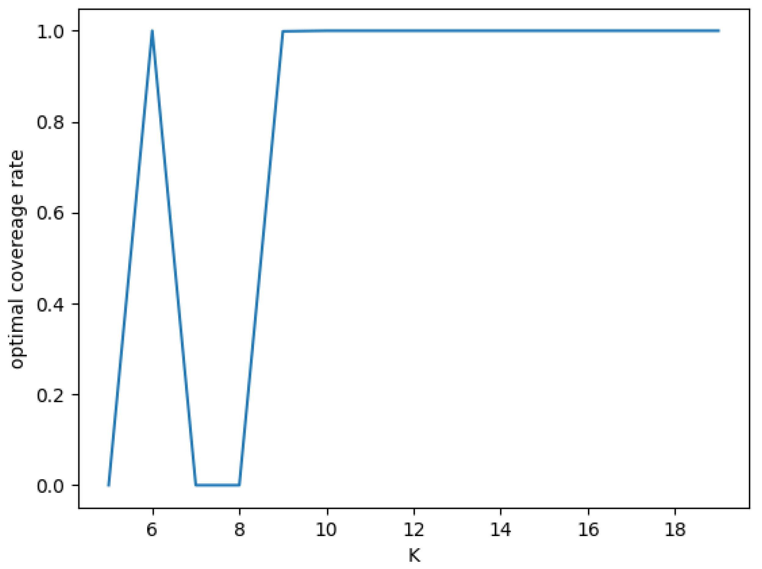
The equilibrium solution was $w^{in*}=0.89\left(0.8863\right)$, $q^{in*}=75\left(75.0\right)$, ${\theta }^{*}=1$, ${\pi }_r=6.29$, and ${\pi }_s^{in}=50.96$. When we conducted the simulation, we retained two decimal places for the profits and the wholesale price.

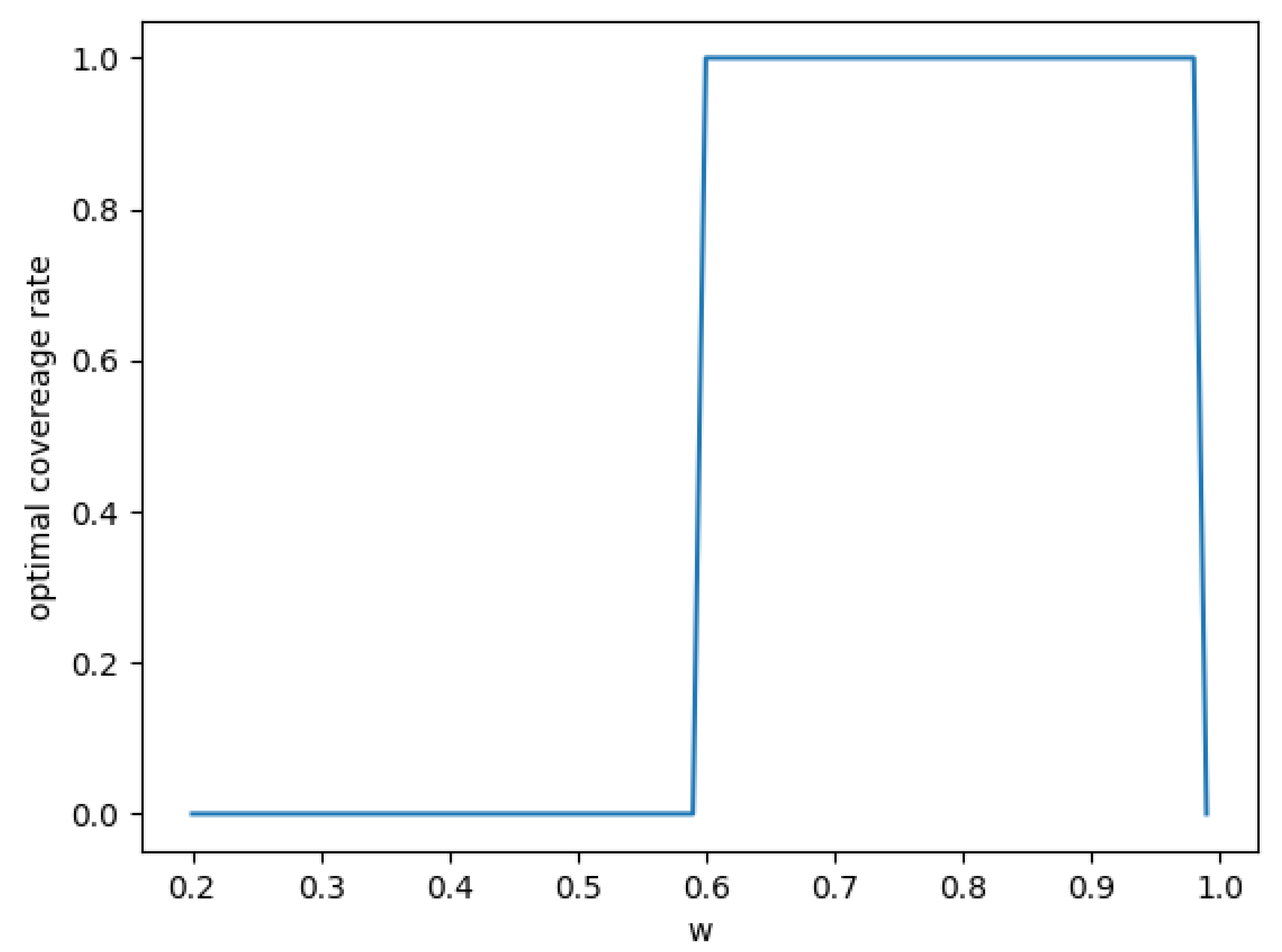
As we can see from Figure 5, as the wholesale price increased, the optimal coverage rate remained at 0 at first. As the wholesale price reached a certain threshold, the optimal coverage rate jumped to 1. Finally as the wholesale price became higher than another threshold, the optimal coverage rate reduced to 0 again.

Now, we determine the relationship between $q^{*}$ and $q^{in*}$ when the exogenous parameters are same, and the retailer needs to use trade credit. We assume that the equilibrium of the no insurance condition is $q=q^{*}$ and $w=w^{*}$. Thus, we have ${\left.\frac{\mathrm{d}{\pi }_s}{\mathrm{d}w}\right|}_{q=q*,w=w^{*}}=0$. If we assume that the capital is sufficient, and the supplier decides to use trade credit insurance, then from Proposition 1, we know that ${\theta }^{*}=1$, and thus

$$\frac{d{\pi }_s^{in}}{d{w}^{in}}=F\left(w^{in}{q}^{in}-K_r\right)\frac{d\left(w^{in}{q}^{in}\right)}{d{w}^{in}}+\left[1-F\left(w^{in}{q}^{in}-K_r\right)\right]\frac{d\left(w^{in}{q}^{in}\right)}{d{w}^{in}}-c\frac{d{q}^{in}}{d{w}^{in}}-s\frac{d\left(w^{in}{q}^{in}\right)}{d{w}^{in}}$$

(17)

Taking ${\left.\frac{\mathrm{d}{\pi }_s}{\mathrm{d}w}\right|}_{q=q*,w=w^{*}}=0$ into (17), we can obtain ${\left.\frac{\mathrm{d}{\pi }_s^{in}}{\mathrm{d}{w}^{in}}\right|}_{q^{in}=q*,q^{in}=w^{*}}<0$. Since, when $\theta =1$, similar to the above, we obtain $\frac{{\mathrm{d}}^2{\pi }_s^{in}}{\mathrm{d}{\left(w^{in}\right)}^2}<0$, then we obtain $w^{in*}<w^{*}$ and $q^{in*}>q^{*}$.

Proposition 4. 

When the trade credit insurance benefits the supplier $({\theta }^{*}>0)$, and the initial capital $(K+K_r)$ is sufficient, we obtain ${\theta }^{*}=1$, $w^{in*}<w^{*}$, and $q^{in*}>q^{*}$.

From Proposition 3, we see that if the supplier can use trade credit insurance, he will buy the total coverage insurance and decrease the wholesale price when the money is sufficient and the insurance premium rate is not high; thus, the retailer will order more. In other words, the trade credit insurance expands the scale of the trade.

However, when the initial capital $(K+K_r)$ is not sufficient, the use of trade credit may reduce the trade quantity. We prove this by using a special case: when D∼$N(100,30)$, $c=0.2$, $K_r=5$, $K=10$, and $s=0.01$, we obtain that if the supplier cannot use trade credit insurance, $w^{*}=0.8899$, $q^{*}=74.5$, ${\pi }_r=6.29$, and ${\pi }_s=50$, and if the supplier can use trade credit insurance $w^{in*}=0.9199$, $q^{in*}=70.7$, ${\pi }_r=4.32$, and ${\pi }_s=50.15$. From the results, we can see that both the order quantity and the expected profit of the retailer decrease. The rationale behind this is that when the initial capital is not sufficient and using trade credit benefits the supplier, he may increase the wholesale price to cause the retailer to order less in order to leave more money $(K+K_r-cq)$ to buy trade credit insurance.

Lemma 2. 

When the initial capital $(K+K_r)$ is not sufficient, having access to trade credit insurance may decrease the trade quantity and the expected profit of the retailer.

This finding is contrary to the conclusion of previous research that trade credit insurance expands trade [7,8,9,10,13].

5. Extension: Supplier with a Potential Financial Cost

According to some of the previous literature [12,40,41,42], if the supplier does not receive enough money from the retailer at the end of the period, he will face a cash flow shortfall. As a result, he may have to obtain money to pay for fixed costs such as rent and salary; thus, he will have external financing costs such as an interest rate premium and a broker fee. So, when we model the supplier’s objective function, we should take the potential financing cost into account. Specifically, we referred to the method used by Yang et al. [12] and assumed that the supplier’s financing cost was $L=l{(T-u)}^{+}$, where u represents the supplier’s end of period net cash flow, which is equal to his revenue minus the manufacturing cost and the insurance premium, (if he uses trade credit insurance). Then, l is the marginal financing cost that the supplier incurs, if u falls short of an exogenous specified threshold T. Thus, for a supplier who does not use trade credit insurance, we will have the subsequent formula:

$$\begin{array}{cc}\hfill {\pi }_s^{{}^{\prime }}& =\mathbb{E}[min\{D,w^{{}^{\prime }}{q}^{{}^{\prime }}-K_r\}+K_r-c{q}^{{}^{\prime }}-l{(T+c{q}^{{}^{\prime }}-K_r-min\{D,w^{{}^{\prime }}{q}^{{}^{\prime }}-K_r\})}^{+}]\hfill \\ \hfill & =\left\{\begin{array}{c}{\int }_0^{w^{{}^{\prime }}{q}^{{}^{\prime }}-K_r}xdF+{\int }_{w^{{}^{\prime }}{q}^{{}^{\prime }}-K_r}^{\infty }(w^{{}^{\prime }}{q}^{{}^{\prime }}-K_r)dF+K_r-c{q}^{{}^{\prime }}(K_r<w^{{}^{\prime }}{q}^{{}^{\prime }},T<K_r-c{q}^{{}^{\prime }})\hfill \\ \\ {\int }_0^{w^{{}^{\prime }}{q}^{{}^{\prime }}-K_r}xdF+{\int }_{w^{{}^{\prime }}{q}^{{}^{\prime }}-K_r}^{\infty }(w^{{}^{\prime }}{q}^{{}^{\prime }}-K_r)dF+K_r-c{q}^{{}^{\prime }}\hfill \\ -l{\int }_0^{T+c{q}^{{}^{\prime }}-K_r}(T+c{q}^{{}^{\prime }}-K_r-x)dF(K_r<w^{{}^{\prime }}{q}^{{}^{\prime }},K_r-c{q}^{{}^{\prime }}\le T\le (w^{{}^{\prime }}-c)q^{{}^{\prime }})\hfill \\ \\ (1+l)[{\int }_0^{w^{{}^{\prime }}{q}^{{}^{\prime }}-K_r}xdF+{\int }_{w^{{}^{\prime }}{q}^{{}^{\prime }}-K_r}^{\infty }(w^{{}^{\prime }}{q}^{{}^{\prime }}-K_r)dF+K_r-c{q}^{{}^{\prime }}]-lT\hfill \\ (K_r<w^{{}^{\prime }}{q}^{{}^{\prime }},T>(w^{{}^{\prime }}-c)q^{{}^{\prime }})\hfill \\ \\ (w^{{}^{\prime }}-c)q^{{}^{\prime }}(K_r\ge w^{{}^{\prime }}{q}^{{}^{\prime }},T\le (w^{{}^{\prime }}-c)q^{{}^{\prime }})\hfill \\ \\ (1+l)(w^{{}^{\prime }}-c)q^{{}^{\prime }}-lT(K_r\ge w^{{}^{\prime }}{q}^{{}^{\prime }},T>(w^{{}^{\prime }}-c)q^{{}^{\prime }})\hfill \end{array}\right.\hfill \end{array}$$

(18)

When $K_r<w^{{}^{\prime }}{q}^{{}^{\prime }}$ and $K_r-c{q}^{{}^{\prime }}\le T\le (w^{{}^{\prime }}-c)q^{{}^{\prime }}$, $\frac{\mathrm{d}{\pi }_s^{{}^{\prime }}}{\mathrm{d}{w}^{{}^{\prime }}}={\left.\frac{\mathrm{d}{\pi }_s}{\mathrm{d}w}\right|}_{w=w^{{}^{\prime }}}-lc\frac{\mathrm{d}{q}^{{}^{\prime }}}{\mathrm{d}{w}^{{}^{\prime }}}F(T+c{q}^{{}^{\prime }}-K_r)$. Since $lc\frac{\mathrm{d}{q}^{{}^{\prime }}}{\mathrm{d}{w}^{{}^{\prime }}}F(T+c{q}^{{}^{\prime }}-K_r)$ is always larger than zero, thus, when $w^{{}^{\prime }}=w^{*}$, ${\left.\frac{\mathrm{d}{\pi }_s}{\mathrm{d}w}\right|}_{w=w^{{}^{\prime }}}=0$, and $\frac{\mathrm{d}{\pi }_s^{{}^{\prime }}}{\mathrm{d}{w}^{{}^{\prime }}}<0$. From the above, we know that $\frac{\mathrm{d}{\pi }_s}{\mathrm{d}w}$ is decreasing with respect to w. So we obtain $q^{{}^{\prime }*}<q^{*}$ and $w^{{}^{\prime }*}>w^{*}$. In other cases, $\frac{\mathrm{d}{\pi }_s^{{}^{\prime }}}{\mathrm{d}{w}^{{}^{\prime }}}={\left.\frac{\mathrm{d}{\pi }_s}{\mathrm{d}w}\right|}_{w=w^{{}^{\prime }}}$, so $q^{{}^{\prime }*}=q^{*}$ and $w^{{}^{\prime }*}=w^{*}$.

Proposition 5. 

When $K_r<w^{{}^{\prime }}{q}^{{}^{\prime }}$ and $K_r-c{q}^{{}^{\prime }}\le T\le (w^{{}^{\prime }}-c)q^{{}^{\prime }}$, $q^{{}^{\prime }*}<q^{*}$ and $w^{{}^{\prime }*}>w^{*}$. In other cases, $q^{{}^{\prime }*}=q^{*}$ and $w^{{}^{\prime }*}=w^{*}$.

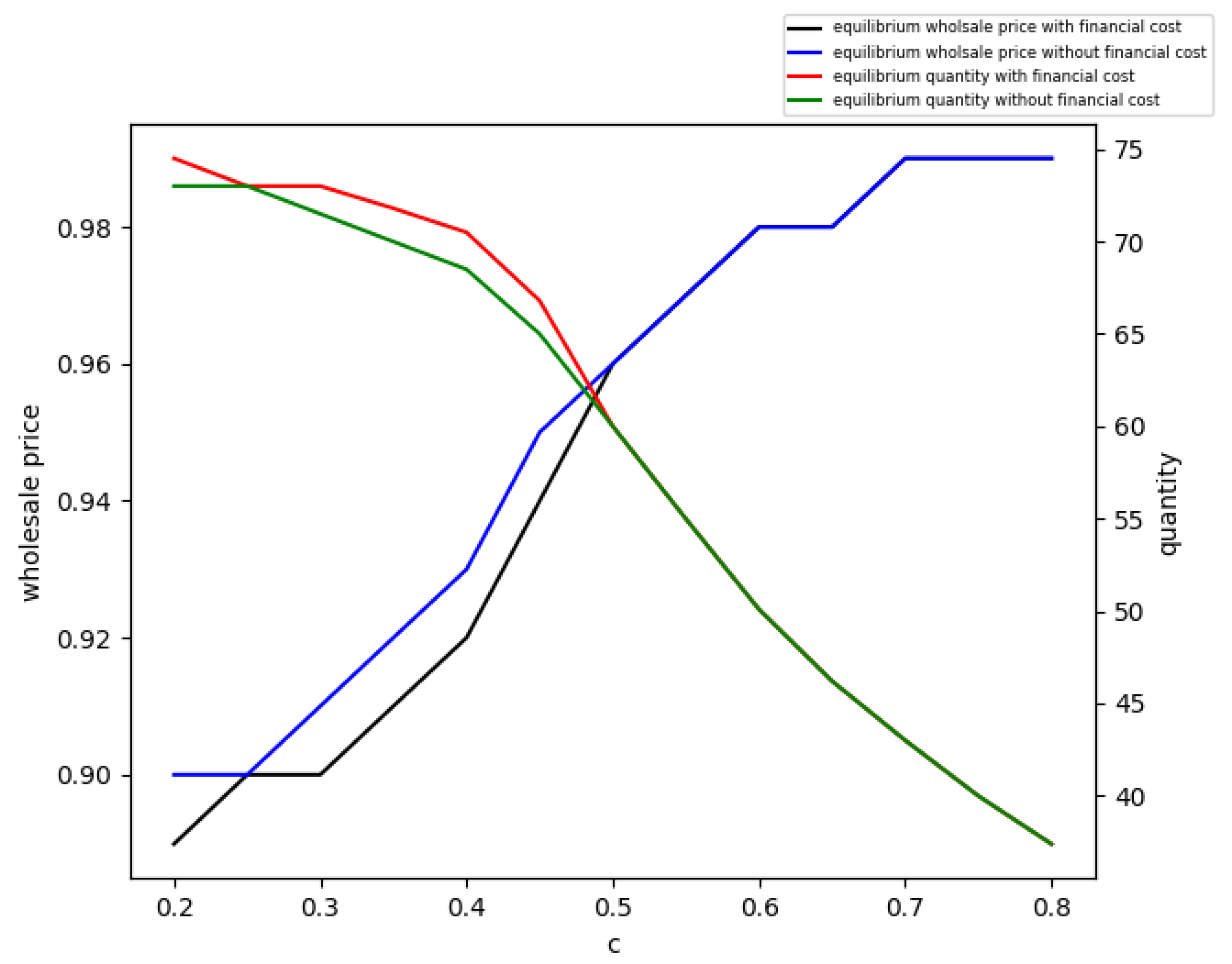
From Proposition 5, we see that if the supplier faces potential financing costs, he may increase the wholesale price; thus, the retailer will order less. In other words, the potential financing cost decreases the scale of trade in some cases and does not affect the scale of trade in the other cases. The effects of the marginal cost on the equilibrium solutions are shown in Figure 8.

When $w^{i{n}^{\prime }}{q}^{in"}<K_r$ and the supplier has access to the trade credit insurance, we have

$$\begin{array}{cc}{\pi }_s^{{}^{\prime }}\hfill & =\mathbb{E}[max\{min\{D,w^{in}{q}^{i{n}^{\prime }}-K_r\},\theta (w^{i{n}^{\prime }}{q}^{i{n}^{\prime }}-K_r)\}+K_r-c{q}^{i{n}^{\prime }}-\theta s(w^{i{n}^{\prime }}{q}^{i{n}^{\prime }}-K_r)\hfill \\ & -l{(T-(max\{min\{D,w^{i{n}^{\prime }}{q}^{i{n}^{\prime }}-K_r\},\theta (w^{i{n}^{\prime }}{q}^{i{n}^{\prime }}-K_r)\}+K_r-c{q}^{i{n}^{\prime }}-\theta s(w^{i{n}^{\prime }}{q}^{i{n}^{\prime }}-K_r)))}^{+}]\hfill \\ & =\left\{\begin{array}{c}{\int }_0^{\theta (w^{i{n}^{\prime }}{q}^{i{n}^{\prime }}-K_r)}\theta (w^{i{n}^{\prime }}{q}^{i{n}^{\prime }}-K_r)dF+{\int }_{\theta (w^{i{n}^{\prime }}{q}^{i{n}^{\prime }}-K_r)}^{(w^{i{n}^{\prime }}{q}^{i{n}^{\prime }}-K_r)}xdF+{\int }_{(w^{i{n}^{\prime }}{q}^{i{n}^{\prime }}-K_r)}^{\infty }(w^{i{n}^{\prime }}{q}^{i{n}^{\prime }}-K_r)dF\hfill \\ +K_r-c{q}^{i{n}^{\prime }}-\theta s(w^{i{n}^{\prime }}{q}^{i{n}^{\prime }}-K_r)(T<K_r-c{q}^{i{n}^{\prime }}+\theta (1-s)(w^{i{n}^{\prime }}{q}^{i{n}^{\prime }}-K_r))\hfill \\ \\ {\int }_0^{\theta (w^{i{n}^{\prime }}{q}^{i{n}^{\prime }}-K_r)}\theta (w^{i{n}^{\prime }}{q}^{i{n}^{\prime }}-K_r)dF+{\int }_{\theta (w^{i{n}^{\prime }}{q}^{i{n}^{\prime }}-K_r)}^{(w^{i{n}^{\prime }}{q}^{i{n}^{\prime }}-K_r)}xdF+{\int }_{(w^{i{n}^{\prime }}{q}^{i{n}^{\prime }}-K_r)}^{\infty }(w^{i{n}^{\prime }}{q}^{i{n}^{\prime }}-K_r)dF\hfill \\ +K_r-c{q}^{i{n}^{\prime }}-\theta s(w^{i{n}^{\prime }}{q}^{i{n}^{\prime }}-K_r)\hfill \\ -l[{\int }_0^{\theta (w^{i{n}^{\prime }}{q}^{i{n}^{\prime }}-K_r)}(T+c{q}^{i{n}^{\prime }}-K_r-\theta (1-s)(w^{i{n}^{\prime }}{q}^{i{n}^{\prime }}-K_r))dF\hfill \\ +{\int }_{\theta (w^{i{n}^{\prime }}{q}^{i{n}^{\prime }}-K_r)}^{T+c{q}^{i{n}^{\prime }}+\theta s(w^{i{n}^{\prime }}{q}^{i{n}^{\prime }}-K_r)-K_r}(T+c{q}^{i{n}^{\prime }}+\theta s(w^{i{n}^{\prime }}{q}^{i{n}^{\prime }}-K_r)-x)dF]\hfill \\ ((1-\theta s)(w^{i{n}^{\prime }}{q}^{i{n}^{\prime }}-K_r)+K_r-c{q}^{i{n}^{\prime }}\ge T\ge K_r-c{q}^{i{n}^{\prime }}+\theta (1-s)(w^{i{n}^{\prime }}{q}^{i{n}^{\prime }}-K_r))\hfill \\ \\ (1+l)[{\int }_0^{\theta (w^{i{n}^{\prime }}{q}^{i{n}^{\prime }}-K_r)}\theta (w^{i{n}^{\prime }}{q}^{i{n}^{\prime }}-K_r)dF+{\int }_{\theta (w^{i{n}^{\prime }}{q}^{i{n}^{\prime }}-K_r)}^{(w^{i{n}^{\prime }}{q}^{i{n}^{\prime }}-K_r)}xdF\hfill \\ +{\int }_{(w^{i{n}^{\prime }}{q}^{i{n}^{\prime }}-K_r)}^{\infty }(w^{i{n}^{\prime }}{q}^{i{n}^{\prime }}-K_r)dF+K_r-c{q}^{i{n}^{\prime }}-\theta s(w^{i{n}^{\prime }}{q}^{i{n}^{\prime }}-K_r)]-lT\hfill \\ (T>(1-\theta s)(w^{i{n}^{\prime }}{q}^{i{n}^{\prime }}-K_r)+K_r-c{q}^{i{n}^{\prime }})\hfill \end{array}\right.\hfill \end{array}.$$

(19)

When $w^{{}^{\prime }}=w^{i{n}^{\prime }}=a$ and $q^{{}^{\prime }}=q^{i{n}^{\prime }}=b$ are given and $K+K_r>cb$, if $K_r-cb\ge T$, we have

$$\begin{array}{cc}\hfill {\theta }^{*}& =\left\{\begin{array}{c}1\left(s\le {\int }_0^{(ab-K_r)}(1-\frac{x}{ab-K_r})dF\mathrm{and}CL\ge 1\right)\hfill \\ CL\left(s\le {\int }_0^{\left(\frac{K+K_r-cb}{s}\right)}(1-\frac{sx}{K+K_r-cb})dF\mathrm{and}CL<1\right)\hfill \\ 0\left(\mathrm{otherwise}\right)\hfill \end{array}\right.,\hfill \end{array}$$

(20)

where $CL$=$\frac{K+K_r-cb}{s(ab-K_r)}$;

if $K_r-cb+\theta (1-s)(ab-K_r)>T>K_r-cb$, we have

$$\begin{array}{cc}\hfill {\theta }^{*}& =\left\{\begin{array}{c}1\left(s\le {\int }_{IP(ab-K_r)}^{(ab-K_r)}(1-\frac{x}{ab-K_r})/(1-IP)dF+F\left[IP(ab-K_r)\right]\mathrm{and}CL\ge 1\right)\hfill \\ CL\left(s\le {\int }_{IP(ab-K_r)}^{CL(ab-K_r)}(CL-\frac{x}{ab-K_r})/(CL-IP)dF+F\left[IP(ab-K_r)\right]\mathrm{and}1\ge CL\ge IP\right)\hfill \end{array}\right.,\hfill \end{array}$$

(21)

where $CL$=$\frac{K+K_r-cb}{s(ab-K_r)}$ and $IP=\frac{T-K_r+cb}{(1-s)(ab-K_r)}$;

if $(1-\theta s)(ab-K_r)+K_r-cb\ge T\ge K_r-cb+\theta (1-s)(ab-K_r)$, we have

$$\frac{d{{\pi }_s^{in}}^{\prime }}{d\theta }=\left(ab-K_r\right)\left\{(1+l)F\left[\theta (ab-K_r)\right]-s-slF[T+cb+\theta s(ab-K_r)-K_r\right]\};$$

(22)

if $(a-c)b\ge T>(1-\theta s)(ab-K_r)+K_r-cb$, we have

$$\begin{array}{cc}\hfill {\theta }^{*}& =\left\{\begin{array}{c}1\left(LB<s\le UB\mathrm{and}CL\ge 1\right)\hfill \\ CL\left(LB/CL<s\le U{B}^{\prime }\mathrm{and}CL<1\right)\hfill \end{array}\right.,\hfill \end{array}$$

(23)

where $CL$=$\frac{K+K_r-cb}{s(ab-K_r)}$; $UB=[{\int }_0^{(ab-K_r)}(1-\frac{x}{ab-K_r})dF+l\frac{(a-c)b-T}{ab-K_r}]/(1+l)$; $LB=\frac{(a-c)b-T}{ab-K_r}$; $U{B}^{\prime }=\{{\int }_0^{CL(ab-K_r)}1-\frac{x}{CL(ab-K_r)}dF-\frac{l(T+cb-K_r)}{CL(ab-K_r)}+l[F\left[CL(ab-K_r)\right]+{\int }_{CL(ab-K_r)}^{ab-K_r}\frac{x}{CL(ab-K_r)}$$dF+{\int }_{ab-K_r}^{\infty }\frac{1}{CL}dF\left]\right\}/(1+l)$;

if $T>(a-c)b$, we have

$$\begin{array}{cc}\hfill {\theta }^{*}& =\left\{\begin{array}{c}1\left(s\le {\int }_0^{(ab-K_r)}(1-\frac{x}{ab-K_r})dF\mathrm{and}CL\ge 1\right)\hfill \\ CL\left(s\le {\int }_0^{\left(\frac{K+K_r-cb}{s}\right)}(1-\frac{sx}{K+K_r-cb})dF\mathrm{and}CL<1\right)\hfill \\ 0\left(\mathrm{otherwise}\right)\hfill \end{array}\right.,\hfill \end{array}$$

(24)

where $CL$=$\frac{K+K_r-cb}{s(ab-K_r)}$.

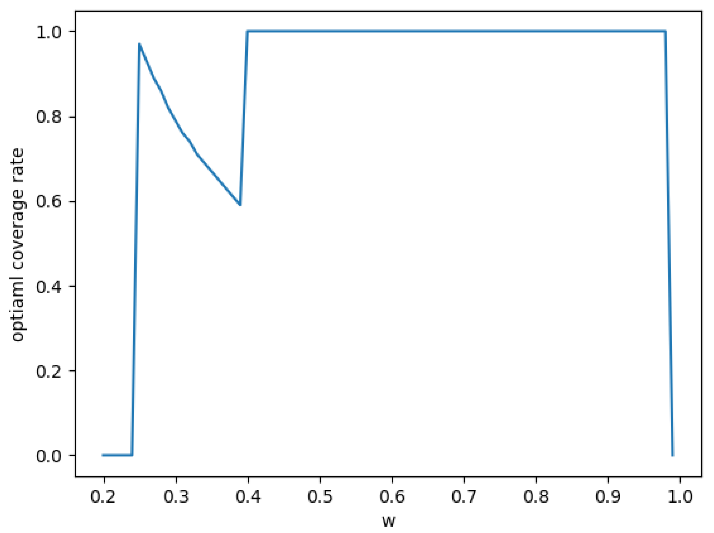
To better illustrate the solutions, we provide Figure 9 and Figure 10, when D∼$N(100,30)$, $c=0.2$, $K_r=5$, $K=25$, $l=30$, $T=5$, and $s=0.01$.

From the equilibrium results, we see that for a capital-constrained supplier, even when the supplier will face potential cost if he does not obtain enough payment, he may decide not to use trade credit insurance at all. Whether the supplier will use trade credit depends on the relationship between the initial capital, the production cost, the market demand distribution, the capital threshold, the marginal financing cost, and the insurance premium rate. If we assume the insurance company has to ensure that its expected return is positive and has no other way to invest the insurance premium, then we obtain

$$\begin{array}{cc}\hfill {\pi }_{ins}& =\theta s(w^{i{n}^{\prime }}{q}^{i{n}^{\prime }}-K_r)-\mathbb{E}{[max\{min\{D,w^{i{n}^{\prime }}{q}^{i{n}^{\prime }}-K_r\},\theta (w^{i{n}^{\prime }}{q}^{i{n}^{\prime }}-K_r)\}-D]}^{+}\hfill \\ \hfill & =\theta s(w^{i{n}^{\prime }}{q}^{i{n}^{\prime }}-K_r)-{\int }_0^{\theta (w^{i{n}^{\prime }}{q}^{i{n}^{\prime }}-K_r)}\theta (w^{i{n}^{\prime }}{q}^{i{n}^{\prime }}-K_r)-xdF>0\hfill \end{array};$$

(25)

thus, $s>{\int }_0^{\theta (w^{i{n}^{\prime }}{q}^{i{n}^{\prime }}-K_r)}1-\frac{x}{\theta (w^{i{n}^{\prime }}{q}^{i{n}^{\prime }}-K_r)}dF$. So, the supplier will never buy trade credit insurance no matter how much the marginal financing cost is when $T\le K_r-c{q}^{i{n}^{\prime }}$ or $T>(w^{i{n}^{\prime }}-c)q^{i{n}^{\prime }}$. This result is different to that of Li’s model [13], where the supplier is risk averse, and a high risk aversion degree will always cause the supplier to use trade credit insurance. We can easily prove that when there is no financial cost, the risk neutral supplier will never buy insurance, if the insurance premium has the mentioned lower bound. However, in practice, the insurance company can invest the insurance premium to earn money. Taking Taikang Insurance Group, one of the largest insurance companies in China, as an example, its return on investment was up to 6.82% in 2021. Therefore, the insurance company does not need to keep the insurance premium rate higher than the abovementioned lower bound.

6. Conclusions

This paper considered a capital-constrained supplier, a capital-constrained retailer, and an insurance company offering trade credit insurance. The retailer faced the stochastic demand of the product with an exogenously fixed price. The retailer might seek trade credit from the supplier, and the insurance company could provide trade credit insurance to the supplier. Given the market demand distribution and the insurance premium, the supplier had to decide the wholesale price and the insurance coverage rate. To the best of our knowledge, this is the first work in the literature on the interface of finance and operations to investigate how a capital-constrained supplier should distribute its capital between the trade credit and the trade credit insurance.

We show that for a capital-constrained supplier, to maximize his profit, he would only choose between not buying the trade credit insurance at all and using all the capital available to buy the insurance (or buy the 100% coverage insurance). When his initial capital was not sufficient, the use of trade credit insurance could reduce the production quantity and the expected profit of the retailer. In other words, when the supplier has limited capital, trade credit insurance may have a negative impact on the expansion of trade, and it is not a win–win choice anymore. This finding was quite different from the previous literature [7,8,9,11,12,13]. However, when the supplier had sufficient initial capital, we used a mathematical model to prove that trade credit insurance would always be beneficial to the expansion of trade.

Even if the supplier faced a potential cost if he did not obtain full repayment, he might decide not to use trade credit insurance at all. Whether the supplier uses trade credit depends on the relationship between the initial capital, the production cost, the market size, the capital threshold, the marginal financing cost, and the insurance premium rate. If the insurance company has to keep its expected return positive and has no other way to invest the insurance premium, then the insurance company has to set an lower bound for the insurance premium. With the lower bound of the insurance premium, the supplier would never buy trade credit insurance no matter how much the marginal potential financing cost would be, if the threshold was too low or too high.

This paper studied the decision-making process of suppliers when they had limited capital and could choose to buy trade credit insurance and identified the optimal strategies of retailers and suppliers in different situations. The paper can help businesses achieve a balance of funds and the logistics of the supply chain and risks, which can improve the effectiveness of the supply chain operation. This paper filled the gap of the capital-constrained supplier in the supply chain insurance-related literature. In addition, the results and methods in this paper provide a decision-making basis for SMEs in reality.

Possible future extensions can include a more universal model that allows competition between multiple retailers and multiple suppliers. It can also deepen the understanding of the problem. However, this may incur undesired mathematical complication and require further techniques.