A Neural Network and Principal Component Analysis Approach to Develop a Real-Time Driving Cycle in an Urban Environment: The Case of Addis Ababa, Ethiopia

Abstract

This study aimed to develop the Addis Ababa Driving Cycle (DC) using real-time data from passenger vehicles in Addis Ababa based on a neural network (NN) and principal component analysis (PCA) approach. Addis Ababa has no local DC for automobile emissions tests and standard DCs do not reflect the current scenario. During the DC’s development, the researchers determined the DC duration based on their experience and the literature. A k-means clustering method was also applied to cluster the dimensionally reduced data without identifying the best clustering method. First, a shape-preserving cubic interpolation technique was applied to remove outliers, followed by the Bayes wavelet signal denoising technique to smooth the data. Rules were then set for the extraction of trips and trip indicators before PCA was applied, and the machine learning classification was applied to identify the best clustering method. Finally, after training the NN using Bayesian regularization with a back propagation, the velocity for each route section was predicted and its performance had an overall R-value of 0.99. Compared with target data, the DCs developed by the NN and micro trip methods have a relative difference of 0.056 and 0.111, respectively, and resolve the issue of the DC duration decision in the micro trip method.

1. Introduction

A driving cycle (DC) is a plot of vehicle speed versus time and is used to assess a vehicle’s performance, emissions, and energy consumption [1]. Various standard DCs, such as WLTC, FTP 75, and JC08, have been created [2]. There is wide agreement among researchers that driving characteristics are unique due to different vehicle fleet compositions, driving behaviors, and roads [3]. The China Light-Duty Vehicle Test Cycle for Passenger Cars (CLTC-P) is close to reality in China, but notably different from other standard DCs based on a comparison analysis [4]. For this reason, existing standard DCs have failed to estimate exhaust pollutants and fuel consumption accurately in various countries. Several studies have therefore focused on constructing DCs using real-world driving data collected on the road. There is no local DC for estimating and testing automobile emissions in Addis Ababa, Ethiopia’s capital city, either for official purposes or for research. Standard DCs do not reflect the current scenario in Addis Ababa.

The typical DC development method used for emissions levels and fuel consumption is the Micro Trip (MT) method [2,5,6], in which several researchers decide on the DC duration based on their experience and previous DC durations. During DC development, they randomly select and chain MTs until the desired DC duration is obtained and repeat this step several times to obtain candidate cycles. The authors of [5] initially opted for a DC duration of between 1200 s and 1300 s and developed two DCs with a duration of 1216 s and 1261 s. To develop the DC for hybrid buses in the city of Zhengzhou in China, Peng et al. (2015) determined the duration of the designed DC to be 1200 s [7]. Similarly, the authors of [6] decided on a DC duration of 1200 s. The authors of [8] developed three DCs for different routes separately, randomly constituting a DC until the required cycle duration was achieved. However, the DCs developed by this method are not repeatable and the cycle length is not representative of actual conditions. Furthermore, the DC duration has an impact on emission and fuel consumption estimates. Adopting a methodology for DC length based on obtained real-time data can therefore be more representative than using conventional DC durations described in the literature. In order to resolve these issues, in the present study a trip-based method of DC development is proposed.

During DC development, the classification method is applied to kinematic segments to cluster them into heterogonous classes based on statistical properties. Several researchers have applied principal component analysis (PCA) using the k-means clustering method [5,6,9,10,11]. The authors of [12] applied PCA to reduce fifteen characteristic parameters to three factor scores, Liu et al. (2018) applied PCA to reduce fifteen kinematic characteristics values to four principal components based on the eigenvalue [10], and Zhou et al. (2017) reduced eight driving parameters to three principal components using PCA [13]. However, there has been no evaluation of which clustering method offers the best performance with PCA. Therefore, in order to identify the best clustering method, a machine classification learner was applied using MATLAB. This trains the model to classify data using supervised machine learning algorithms. All classification learner methods available were applied to the input dataset, and the algorithms then computed the accuracy scores using the observations.

Machine learning currently offers the best theoretical foundation for DC prediction with deep learning [14]. Chen et al. (2019) used a DC prediction method based on a convolutional neural network [15], while Qiu et al. (2018) used a recurrent neural network-based technique to develop DCs for light-duty vehicles in Beijing [16]. To improve fuel economy, Zhao et al. (2018) proposed a deep reinforcement learning framework for hybrid electric vehicle power control [17].

Inspired by the recent breakthrough in machine learning, this study proposes the use of principal component analysis (PCA) and neural network (NN) prediction methods to develop a DC. To demonstrate the significance of the proposed methodology in this study, the authors also developed the DC using the MT method using the same data used for the NN method. Then, the authors compared the developed DCs with processed experimental (target) data using characteristic parameters to evaluate their representativeness. The real-time driving data used in this study were taken from five vehicles using a global positioning system (GPS) in Addis Ababa city. By means of MATLAB, outliers were found and filled in using shape-preserving cubic interpolation (PCHIP), then the Bayes wavelet signal denoising technique was used to remove noise from the data. Subsequently, seventeen trip indicators were generated for each trip after the denoised data were separated into trips based on predetermined criteria. The dimensions of the trip indicators were then reduced using PCA. After the NN clustering divided the trips into highly diverse categories, the best trip selection followed. In order to train the NN to predict the vehicle speed for each road type, Bayesian regularization with a back-propagation training algorithm was used. The predicted speeds were then joined to generate a representative Addis Ababa DC.

The main aim of this project was to create the Addis Ababa DC using real-time data from passenger vehicles. The Addis Ababa DC was developed based on the data collected, evaluating their characteristic indicators and comparing them with the produced cycle and standard DCs. The analysis results indicate that the developed Addis Ababa DC using NN prediction is more representative of real-time collected data than the MT method and is significantly different from standard DC characteristic parameters.

2. Materials and Methods

2.1. Study Area

Addis Ababa has a total population of 5,227,794 urban and rural inhabitants and is growing at a rate of 4.42% [18]. Addis Ababa has five main entry and exit roads to neighboring cities such as Akaki, Sendafa, Sululta, Holeta, and Sebeta. Addis Ababa’s road network is greatly affected by topographic changes, resulting in positive uphill and negative downhill slopes, with an average road gradient of almost 4% [19]. Addis Ababa’s main roads to different parts of the country and live traffic retrieved from Google Maps on 25 September 2021 are shown in Figure 1.

The city is plagued by severe traffic congestion, which exacerbates vehicle emissions. Tarekegn and Gulilat (2018) discovered that the vehicle growth rate is 9.88% per year, while the road network expansion rate is 8.22%, and they counted 168 vehicles along a one-kilometer stretch of a single-lane asphalt road [20]. In 2020, there were 596,084 vehicles in Addis Ababa city [19], while 627,460 vehicles were registered there [13]. Passenger cars, light commercial vehicles, heavy-duty vehicles, motorcycles, and buses account for 41%, 34%, 18%, 3.96%, and 2.99% of vehicles, respectively [14]. Of the vehicles registered in the city, 43.43% are petrol and 56.57% are diesel-fueled vehicles [20]. Just over half (53.5%) of the vehicles in Addis Ababa city are over 20 years old, while 29.3% are over 30 years old [21]. This indicates that most cars have exceeded their usable service life and are heavily polluting the city. For the majority of citizens, city buses and minibus taxis are accessible, economical modes of public transport [19]. Congestion, delays, and stress on individuals are caused by the city’s poor transport infrastructure, which results in more traffic accidents [22].

2.2. Data Collection and Setup

As a paradigm for DC development, the primary driving data were collected from Addis Ababa, Ethiopia. Raw data from 7442.203 km of driving data were collected from 1 October 2021 to the end of December that year using on-board diagnosis (OBD) II-based GPS devices installed on Toyota Corollas, Tacoma and 5L mini-buses, and Hyundai and Isuzu mid-buses registered and travelling in Addis Ababa city. The entire set of collected data for modeling comprised 1,893,256 s of speed-time points. The real-time driving data logged from the installed GPS devices were timestamp, latitude and longitude, vehicle speed, number of satellites used for data collection, location name at each timestamp, and ignition switch position. Data collection periods included working days and weekends, and the drivers were allowed to travel as they usually did on their day-to-day journeys.

The data collection devices used in this study collected geographical locations with their local names according to Google Map naming. The location names were carefully checked with Google Maps. Based on the identified location name and experience, data collected from the Addis–Adama expressway and ring roads in Addis Ababa city were easily separated. When evaluated, almost every trip covered urban, extra-urban, and rural roads, but ring road and expressway data were only available for some trips. Therefore, ring road and expressway data points were removed from the trip analysis. After removing outliers, de-noising the data points, and removing driving data out of Addis Ababa city, urban roads covered 4895.43 km, rural roads covered 1505.14 km, ring roads covered 475.28 km, and the expressway covered 566.35 km. Figure 2 shows the percentage of distance traveled on each road type.

2.3. DC Development Method

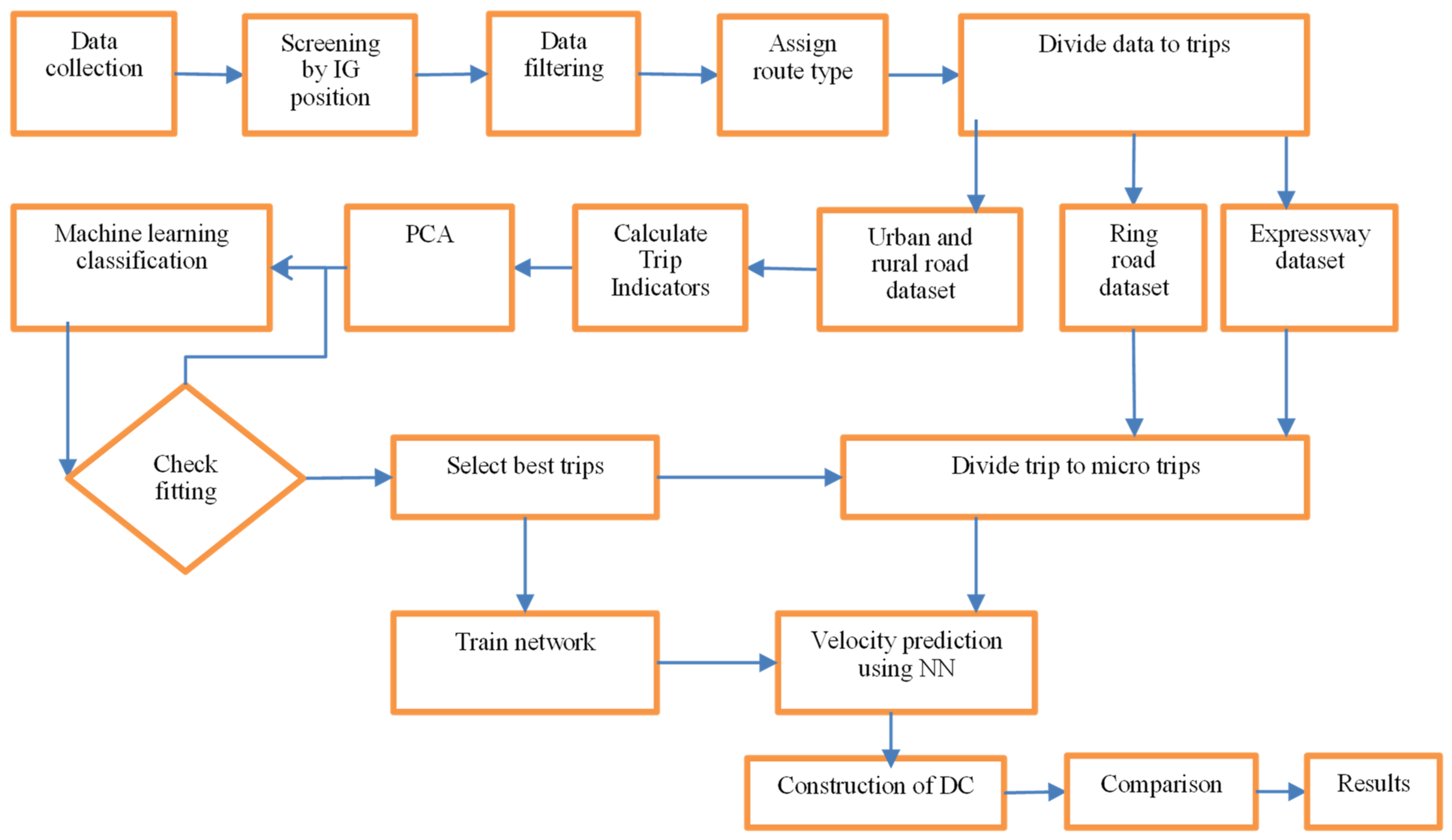
This section covers the methodological aspects of DC development. The methodology adopted in this part of the study included a literature review, vehicle selection, data collection, and an evaluation of the results. DCs were obtained using the trip methods with neural-network-based prediction after trips were classified by means of principal component analysis. Moreover, a DC utilizing the micro trip method from the same data used for the NN prediction method was developed to demonstrate the significance of the methodology provided in this study. There are three critical components in the development of a DC: vehicle selection, data collection, and cycle construction. The various steps in real-time DC development are outlined in Figure 3. Finally, the ability of the obtained DCs to represent the driving conditions in Addis Ababa using characteristic parameters was assessed.

2.4. Data Filtration

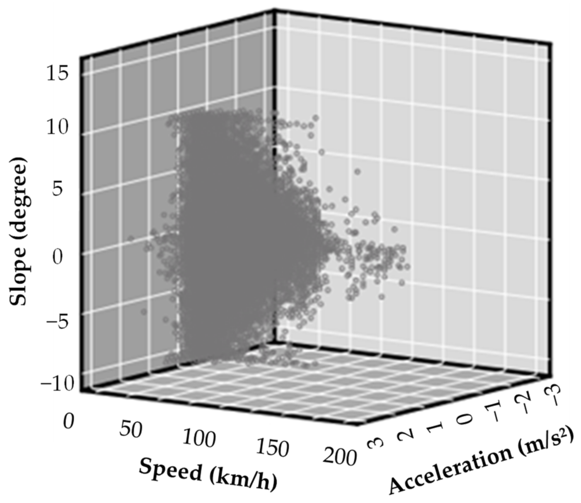
Considering possible GPS errors caused by vibration, the data points with acceleration above 4.5 m/s² and below −4.5 m/s² were removed at the start of data processing based on the WLTC standard. The speed, acceleration, and road slope distribution of the original data are shown in Figure 4.

Before denoising the speed, road grade, and distance of the data collected, time stamps were converted to serial time using MATLAB. Outliers were identified using shape-preserving cubic interpolation (PCHIP) by implementing the moving mean window-centered method. After filling outliers, the noise had to be removed from the collected raw data using the Bayes wavelet signal denoising method.

Then, speed values below 3.6 km/h were changed to 0 km/h to remove the error due to the data collection device, and speed values above 120 km/h were adjusted to 120 km/h because the maximum speed allowed in Ethiopia is 120 km/h. The 974 data points of road grade that were above 10 degrees were adjusted to 10 degrees, and the 1078 data points that were below −10 degrees were adjusted to −10 degrees. Finally, to complete the data denoising process, acceleration was determined for each point of filtered speed data and checked for maximum and minimum values. The maximum and minimum acceleration values were 2.486 m/s² and −2.45 m/s², respectively. Excessive idle times were adjusted to a duration of three minutes [5].

2.5. Neural Network (NN) Prediction Method of DC Development

2.5.1. Approach to Developing the Trip-Based Model

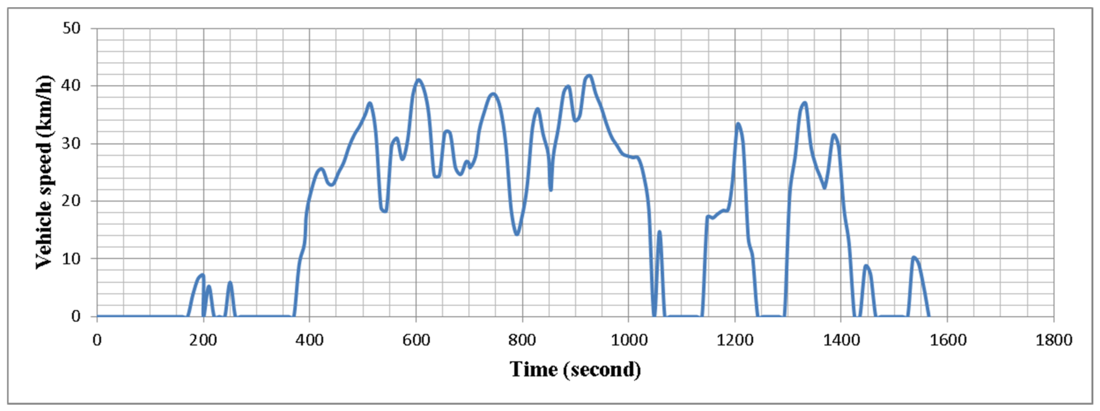
A trip is defined here as a driving process from an origin to a destination with a short stop duration. This may include driving from home to the workplace with a preceding short parking time. Real-world driving trips may contain long and short parking durations, with multiple starts and stops between the origin and the final destination for different reasons, such as vehicle users planning multiple activities to be performed within a single trip and traffic accidents. The collected driving data were segmented into numerous trips based on a parking (stop) duration longer than 30 min, but parking duration was not used in the subsequent analysis. From the collected data, the speed and time plot for one sample trip is shown in Figure 5.

A stop duration of over 30 min was considered to be a cut-point of the trip, which means that if the stop duration is less than 30 min the vehicle has not reached its final destination point and a stop of this kind will be due to congestion, an accident on the road, shopping, etc., and then the trip will continue. Based on this assumption, the screened data were classified into trips and a trip code was assigned to each trip.

A MATLAB program was used to divide the experimental data into trips. In all, 726 trips were obtained (data on 273, 126, 134, 86, and 107 trips were collected from Toyota Corollas, Tacoma and 5L mini-buses, and Hyundai and Isuzu mid-buses, respectively). In this study, based on the common practice of DC development, 17 trip indicators or assessment parameters were selected. In contrast to average speed, which includes idling phases, average driving speed is the mean of the vehicle running speed excluding idle periods. A vehicle’s speed and acceleration are directly related to the amount of power the engine needs to move it forward. The load put on the engine cannot be adequately described by a single variable. However, the best measurement is provided by combining them. Therefore, the trip indicators relative positive acceleration (RPA) and positive kinetic energy (PKE) were used. RPA is the integral of the instantaneous speed and positive acceleration product across a specific trip section. PKE is the sum of differences between the squares of the final and initial speeds in successive accelerations, divided by the distance traveled. These are shown in

Table 1. Trip indicators.

S/N	Trip Indicators	Abbreviation	Unit
1	Driving time	Ttotal	s
2	Distance traveled	Ssum	m
3	Average driving speed	Vdavg	km/h
4	Average speed	Vavg_all	km/h
5	Maximum speed	Vmax	km/h
6	The standard deviation of speed	Vsd
7	Average acceleration	aavg	m/s2
8	Maximum deceleration	decmax	m/s2
9	Maximum acceleration	amax	m/s2
10	The standard deviation of acceleration	asd	m/s2
11	Stop per kilometer	Nspkm	/km
12	Relative positive acceleration	RPA	m/s2
13	Positive kinetic energy	PKE	m/s2
14	Percentage of idle mode	Pidl	%
15	Percentage of acceleration mode	Pacc	%
16	Percentage of cruising mode	Pcru	%
17	Percentage of deceleration mode	Pdec	%

.

Seventeen trip indicators or assessment statistics were then computed for the data from each of the 726 trips. Vehicle speed, time, and distance traveled were collected directly, but for any given time point the value of acceleration was determined according to the WLTP standard. Then, based on the value of acceleration, the following driving modes were determined: idle (velocity is zero), acceleration (greater than 0.1 m/s²), deceleration (less than −0.1 m/s²), and cruising state (between −0.1 and 0.1 m/s²) [8].

To select the most valuable data points, frequency and cumulative frequency were determined for all 726 trips to remove very short trips from further analysis. Trips of less than 540 s or that covered a distance of less than 500 m were removed. Data from 199 short trips were not used in the subsequent analysis due to their limited information that could have led to incorrect interpretations.

As previously stated, the collected datasets should include diverse characteristics for various route types in terms of different times of day, days of the week, and districts served. Therefore, a cluster analysis technique was employed to classify the 527 trips based on the 17 trip indicators. The number of variables in the data reduces the computational efficiency and undermines the clustering effect [5]. Thus, 17 trip indicators was too many and therefore the dimensions were reduced by means of principal component analysis.

2.5.2. Principal Component Analysis (PCA)

PCA is a method that transforms a set of complex variables into a few principal components [6,13]. PCA refers to combining original parameters into a new set of uncorrelated comprehensive parameters for analysis, rather than using the original parameters [7,23]. As mentioned in [5], the PCA method simplifies data and obtains results with more effective information. When PCA is applied for decomposition, the common factors F = (F₁, F₂, …, F_n) and the original variables are modeled as linear combinations of common factors. Generally, a transformation method such as Varimax rotation is used to improve the interpretation of the results through the rotation of factors in a multidimensional space to utilize the best-simplified structure [24].

In this study, Eigen decomposition and Varimax rotation were used with the Kaiser Normalization methods. After reducing the dimension, trips were divided using the clustering method.

2.5.3. Trip Clustering

The groupings are built to be as statistically different as possible between groups and as statistically homogeneous as possible within a group [8]. Different clustering methods can develop different clustering solutions; therefore, to identify the best clustering method, a classification learner was applied using MATLAB. This trains models to classify data using supervised machine learning algorithms. All of the available classification learner methods are applied to the input dataset, and then the algorithms compute the accuracy scores using the observations. This also creates predictions based on these observations and calculates the confusion matrix and ROC curve accordingly. After training a model in the classification learner, the model’s performance or validation accuracy score is compared with the trained data, which aids in the selection of the appropriate clustering strategy. The trip clustering method was chosen based on the results of the classification learner, as we selected the method with the highest validation accuracy. In this study, neural network clustering performed better than the other methods.

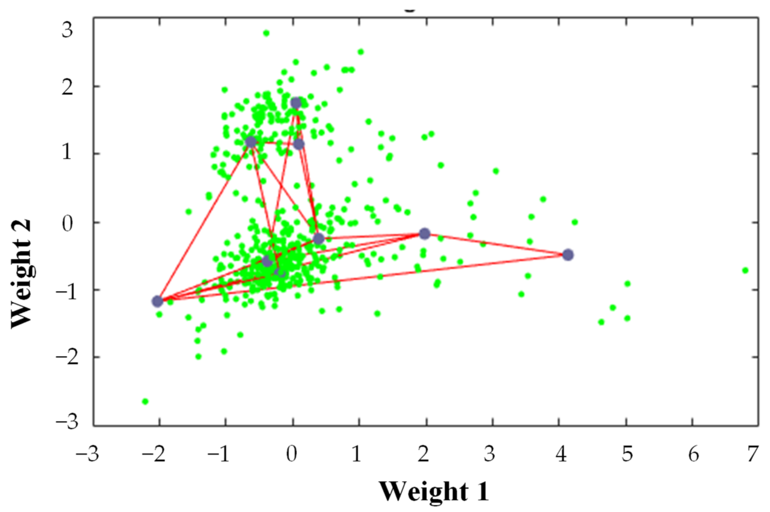
Neural network clustering is a technique that uses a self-organizing map to train a neural network on patterns such that the network can classify them based on their similarity and relative topology. A self-organizing map consists of a competitive layer that can classify a dataset of vectors with any number of dimensions into as many classes as the layer’s neurons. The neurons are placed in a 2D topology, allowing the layer to represent the distribution and approximate the topology of the dataset in two dimensions. As depicted in Figure 6, the factor scores (FACs) of all trips were classified using the neural network clustering technique, which employs a self-organizing map to train a neural network based on batch weight rules, after the dimension of the 17 trip indicators was reduced to five dimensions of FACs using PCA. This network divided the inputs (5 FACs of 527 trips) into 9 classes (output). After the applied clustering technique divided the trips into significantly different groups, the best trip selection followed.

2.5.4. Selection of the Best Trip

Given the input information, appropriate trips were selected based on a calculated similarity score for each cluster. The similarity score was based on the sum of relative errors between the indicators of the candidate trips and the target DC. Given the values of target cycle indicators, the relative error of each indicator of the candidate trip was calculated for each group in accordance with Equation (1):

$${\epsilon }_{\beta k}=\left|\frac{\left(M_{\beta k}-\overline{M_k}\right)}{\overline{M_k}}\right|$$

(1)

where

ε_𝛽𝑘 = the relative error for the kth parameter of candidate trip β, where β is the number of candidate trips and k = 1, 2, …, N, where N is the total number of trip indicators,

𝑀_𝛽𝑘 = the magnitude of the kth trip indicator of the candidate trip β, and

𝑀̅_𝑘 = the mean of the kth trip indicator (the target trip).

Then, the similarity score of a candidate trip could be calculated in accordance with Equation (2):

$$S_{\beta }=1-\frac{1}{N}\left({\displaystyle \sum _{k=1}^N{ϵ}_{\beta k}}\right)$$

(2)

where 𝑆_𝛽 is the similarity score for candidate trip β.

The similarity score was calculated using 1 minus the average relative errors coming from the indicators of candidate trip β. The score ranges from 0 to 1 (where 1 means no errors and fully matches the target cycle). The candidate trip with the highest score is the best trip that matches the provided input information to the greatest extent. It should be noted that the trip indicators were treated equally in the calculation. The trip that best matched the trip-level indicators was selected as the best trip.

The best trips from each cluster were divided into micro trips (MTs). An MT is a driving sequence between two idling events [2]. WLTC standards were followed to divide the driving sequence into MTs for the selected best trips and ring road and expressway data points. Each MT was then assigned a code name. Finally, based on the relative error, the two best MTs were selected that best represented their cluster. Additionally, in order to include ring road and expressway data points in the final DC, one MT from each was chosen. The selected MTs were arranged in a time series sequentially as urban, extra-urban, rural, ring road, and expressway parts.

2.5.5. NN-Based Vehicle Speed Prediction

Prediction is a kind of dynamic filtering in which past values of one or more time series are used to predict future values. Dynamic neural networks, which include delay-line taps, are used for nonlinear filtering and prediction. In a study to develop a DC for light-duty vehicles in Beijing, a recurrent NN approach was adopted [16]. The authors of [15] predicted a DC using a convolutional NN and [25,26] established a DC recognizer using an NN algorithm. The NN model divides the target time steps into training, validation, and testing datasets. The network randomly assigns 70%, 15%, and 15% of the target time steps to the training, validation, and testing datasets, respectively. A nonlinear autoregressive with external input (NARX) model as shown in Equation (3) was applied to predict the output Y(t).

$$\mathrm{Y}\left(\mathrm{t}\right)=\mathrm{f}\left(\mathrm{x}\left(\mathrm{t}-1\right),\dots ,\mathrm{x}\left(\mathrm{t}-\mathrm{d}\right),\mathrm{y}\left(\mathrm{t}-1\right),\dots ,\mathrm{y}\left(\mathrm{t}-\mathrm{d}\right)\right)$$

(3)

where Y(t) is the predicted vehicle speed at time t (output), d is the past speed value of Y(t), x(t) is the collected vehicle speed series of MTs of the respective route (input data), and y(t) is the speed series of the best selected MTs defining the desired output (targets).

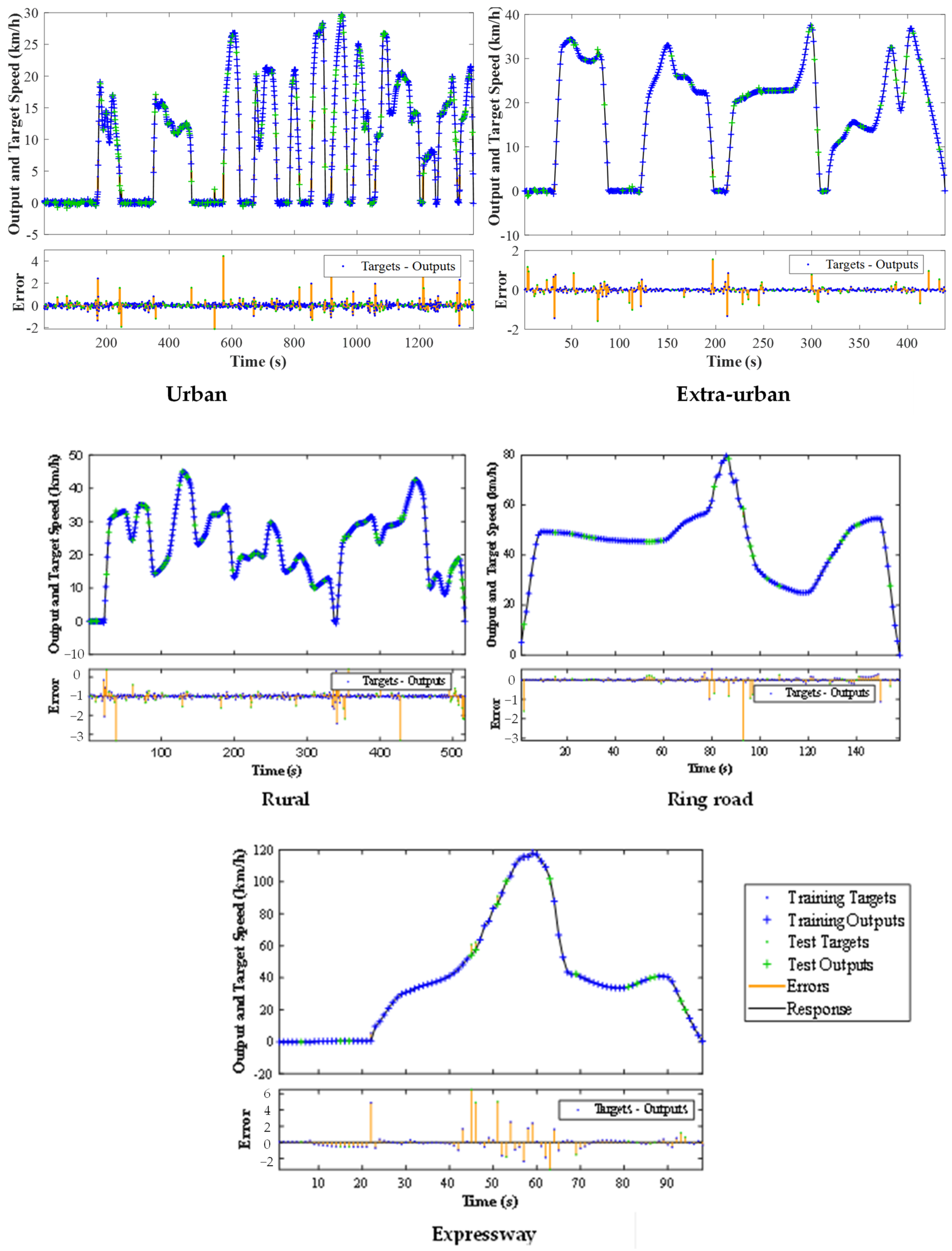
All trip data were converted to a time series and used as the training data (input data) of their route, and the selected MTs from each route were used as the test data (target) during the application of the NN. A sigmoid transfer function was used in the hidden layer of the applied NARX network model (Figure 7), and a linear transfer function was used in the output layer. The NARX network’s output provides feedback to the network’s input. Ten hidden neurons were used during the training.

Bayesian regularization with a back-propagation training algorithm was applied to train the network. Although this technique takes longer, it can provide a high level of generalization for complex, tiny, or noisy datasets. Training stops were based on adaptive weight minimization (regularization). The NN-predicted speed value from each road category was combined to construct a representative DC. Finally, the developed AADC was compared to the DC developed using the micro trip (MT) method, collected data, and standard DCs.

2.6. Micro Trip Method of DC Construction

The best method for building DCs is the micro trip (MT) method [2,27]. We created a DC utilizing the MT approach using the same data used for the NN prediction method to demonstrate the significance of the methodology provided in this study. The driving characteristic parameters were calculated after the speed time data were denoised and segmented into MTs. Using MATLAB, 9451 MTs were obtained from the data. The very lengthy MTs (longer than 1000 s) and very short MTs with very few driving points (less than 30 s) were excluded. With the help of the K-means clustering algorithm, the remaining 6680 MTs were grouped into six clusters. The closest MT to cluster centers is chosen as the typical MT in order to create a DC from each cluster. Until the time sharing requirement is satisfied, the MT selection procedure continues until enough MTs are selected from each cluster. The proportion of each cluster or traffic condition in the final DC is proportional to the duration of that condition in the collected data. Based on the WLTC and the present DC durations, we decided to use a DC duration between 1500 s [28] and 1800 s [4].

The representativeness of the driving pattern contained in the candidate DC was evaluated. The driving patterns in the collected driving data and contained in the clustered group were described by a set of characteristics parameters (CPs), which are also called target parameters. Then, the candidate DC was also described by its characteristic parameter (CP*). Finally, we established that a DC represents a driving pattern when the characteristic parameters of the candidate DC are approximately similar to the target parameters. Thus, the degree of representativeness of a candidate DC was evaluated as the relative difference between paired CPs according to Equation (4) [27].

$${\mathrm{RD}}_{\mathrm{i}}=\frac{\left|{\mathrm{CP}}_{\mathrm{i}}-\left.{\mathrm{CP}}_{\mathrm{i}}^{*}\right|\right.}{{\mathrm{CP}}_{\mathrm{i}}}$$

(4)

During a cycle’s development, the maximum acceptable difference among the paired CPs is 15% [29]. The process of obtaining a candidate DC is repeated several times until an acceptable threshold is obtained. The candidate DC that fulfils this threshold becomes the representative DC. Using this approach, we produced different candidate DCs. From among these, we selected the best one that had the least paired CPs and compared it to the processed experimental data and the DC developed by the NN prediction method.

3. Results

Once the two methods presented above had been employed, we obtained their respective DCs and assessed how closely the obtained DCs reflected the data collected in real time.

3.1. NN Prediction Method

To reduce the dimension of the trip indicators, we applied principal component analysis (PCA) using SPSS 26 on all trip indicators from 527 trips. A correlation test was applied before the PCA analysis. The KMO (a measure of sampling adequacy) was found to be greater than 0.7 and the significance was zero, as shown in

Table 2. KMO and Bartlett’s test.

Kaiser–Meyer–Olkin Measure of Sampling Adequacy		0.709
Bartlett’s Test of Sphericity	Approx. Chi-Square	9288.263
	df	136
	Sig.	0.000

, indicating that the sample collected was sufficient for PCA analysis.

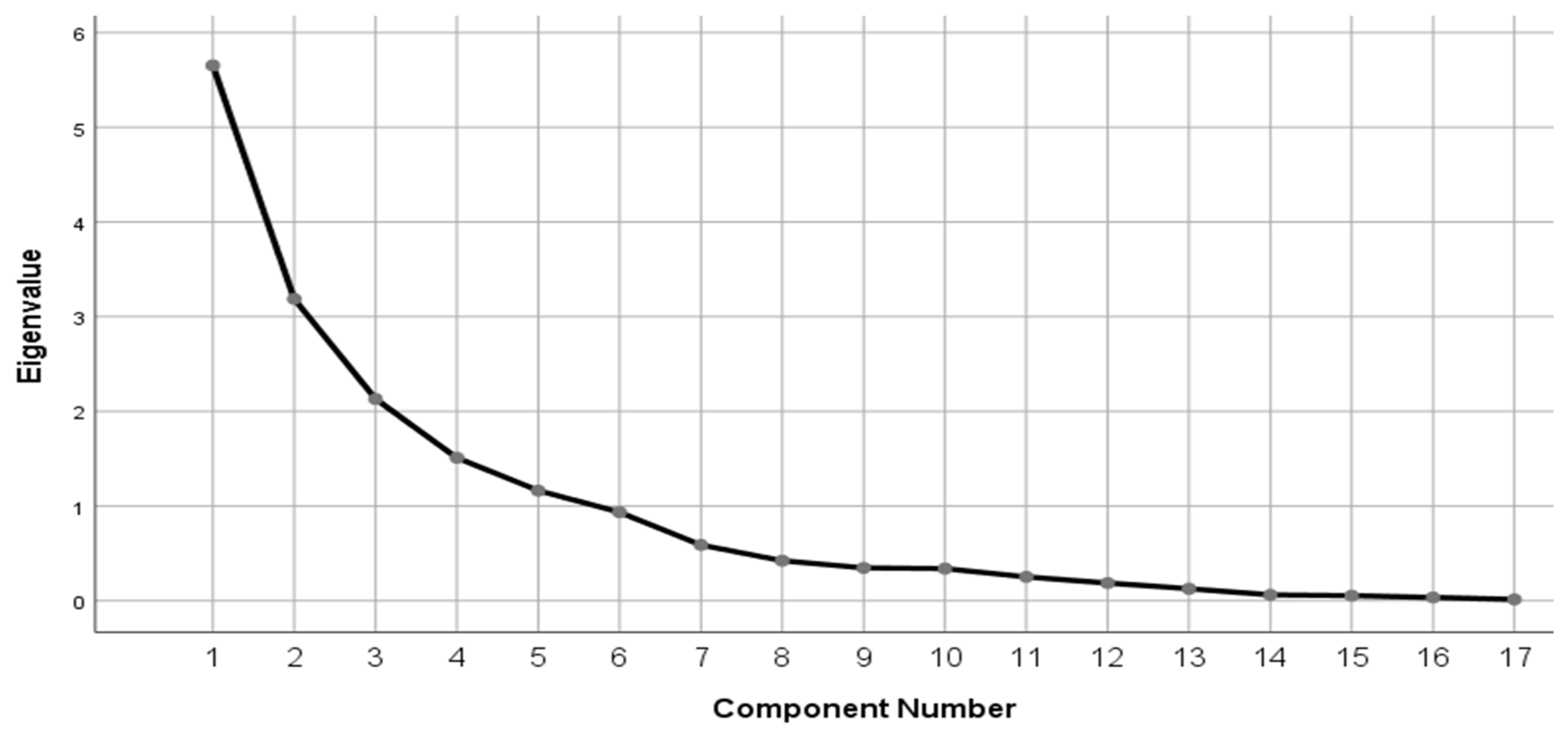
Components 1, 2, 3, 4, and 5 had an eigenvalue above 1 and the cumulative percentage of variance was 80.247%, indicating that important information was included. As mentioned in [12], a cumulative contribution greater than 80% is acceptable. Components that had an eigenvalue of less than 1 were ignored as they did not contain sufficient information. The component matrix obtained is shown in

Table 3. Total variance.

Component	Initial Eigenvalues			Extraction Sums of Squared Loadings			Rotation Sums of Squared Loadings
	Total	% of Variance	Cumulative %	Total	% of Variance	Cumulative %	Total	% of Variance	Cumulative %
1	5.652	33.249	33.249	5.652	33.249	33.249	3.648	21.459	21.459
2	3.187	18.748	51.997	3.187	18.748	51.997	3.48	20.469	41.928
3	2.13	12.531	64.528	2.13	12.531	64.528	2.861	16.828	58.756
4	1.51	8.88	73.408	1.51	8.88	73.408	2.143	12.608	71.364
5	1.163	6.839	80.247	1.163	6.839	80.247	1.51	8.883	80.247
6	0.934	5.495	85.742
7	0.588	3.46	89.202
8	0.422	2.484	91.686
9	0.347	2.039	93.724
10	0.339	1.993	95.717
11	0.252	1.482	97.199
12	0.187	1.098	98.297
13	0.126	0.743	99.04
14	0.062	0.364	99.404
15	0.053	0.311	99.716
16	0.034	0.202	99.918
17	0.014	0.082	100

and the eigenvalue scree plot is displayed in Figure 8.

The score of the five rotated component matrices depicted in

Table 4. Rotated component matrix.

Indicators	F1	F2	F3	F4	F5
Vdavg	0.888	0.126	−0.215	0.113	0.023
Vmax	0.869	0.149	−0.001	0.264	0.144
Vsd	0.833	0.003	−0.007	0.144	−0.052
Vavg_all	0.754	0.089	−0.565	0.083	0.035
Ssum	0.673	0.204	−0.121	0.016	0.626
Pdec	0.068	0.941	−0.127	0.05	0.158
Pacc	0.204	0.82	−0.291	0.218	0.076
aavg	0.086	−0.766	−0.142	0.444	−0.178
PKE	0.193	0.673	0.414	0.345	−0.203
asd	0.222	0.579	0.038	0.442	−0.1
Pidl	−0.079	−0.12	0.947	0.005	0.049
Pcru	0.08	−0.403	−0.852	−0.065	−0.051
Nspkm	−0.285	−0.337	0.723	−0.141	0.003
amax	0.216	−0.032	0.032	0.904	0.125
decmax	−0.174	−0.269	0.088	−0.781	−0.226
Ttotal	0.265	0.3	0.182	0.06	0.785
RPA	−0.083	−0.082	−0.017	0.122	0.539

clearly shows the trip indicators clustered on the basis of their similarities. Factor one (F1) includes velocity and distance-related indicators, factor two (F2) includes the proportion of acceleration and deceleration time, the PKE, and the average and standard deviation of acceleration, factor three (F3) includes stop-related indicators and the percentage of constant speed driving, factor four (F4) includes maximum acceleration and deceleration, and factor five (F5) includes RPA and trip duration.

The trip data matrix and the rotated component matrix for each trip were multiplied as stated in Equation (5) to produce the scores of component matrices (FACs). Scores of the five principal components were taken as the research object for clustering.

FAC_1 = 0.888V_davg + 0.869V_max + 0.833V_sd + 0.754V_{avg_all} + 0.673S_sum + 0.068P_dec + 0.204P_acc

+ 0.086a_avg + 0.193PKE + 0.222a_sd − 0.079P_idl + 0.08P_cru − 0.285N_spkm + 0.216a_max

− 0.174dec_max + 0.265T_total − 0.083RPA

FAC_2 = 0.126V_davg + 0.149V_max + 0.003V_sd + 0.089V_{avg_all} + 0.204S_sum + 0.941P_dec + 0.82P_acc

− 0.766a_avg + 0.673PKE + 0.579a_sd − 0.12P_idl − 0.403P_cru − 0.337N_spkm − 0.032a_max

− 0.269dec_max + 0.3T_total − 0.082RPA

FAC_3 = −0.215V_davg − 0.001V_max − 0.007V_sd − 0.565V_{avg_all} − 0.121S_sum − 0.127P_dec − 0.291P_acc

(5)

−0.142a_avg + 0.414PKE + 0.038a_sd + 0.947P_idl − 0.852P_cru + 0.723N_spkm + 0.032a_max

+ 0.088dec_max + 0.182T_total − 0.017RPA

FAC_4 = 0.113V_davg + 0.264V_max + 0.144V_sd + 0.083V_{avg_all} + 0.016S_sum + 0.05P_dec + 0.218P_acc

+ 0.444a_avg + 0.345PKE + 0.442a_sd + 0.049P_idl − 0.065P_cru − 0.141N_spkm + 0.904a_max

− 0.781dec_max + 0.06T_total + 0.239RPA

FAC_5 = 0.023V_davg + 0.144V_max − 0.052V_sd + 0.035V_{avg_all} + 0.626S_sum + 0.158P_dec

+ 0.076P_acc − 0.178a_avg − 0.203PKE − 0.1a_sd + 0.049P_idl − 0.051P_cru + 0.003N_spkm

+ 0.125a_max − 0.226dec_max + 0.785T_total + 0.239RPA

3.1.1. Clustering Result Analysis

After training a model in a classification learner, the model’s performance or validation accuracy score is checked against the trained data, helping with the selection of the best model. MATLAB software was used to calculate the accuracy score of the classification learning techniques. The accuracy score is represented as the proportion of true results (true positives and negatives) divided by the total number of cases examined (true positives, false positives, true negatives, and false negatives). The accuracy score results of the input data are summarized in

Table 5. Accuracy score of classification learner methods.

S/N	Methods	Accuracy (Validation)
1	Decision trees	63.9–71.3%
2	Discriminant analysis	65.0–82.0%
3	Naïve Bayes classifiers	61.3–71.2%
4	Support vector machines	68.5–85.2%
5	Nearest neighbor classifiers	71.3–74.4%
6	Neural network classifier	82.9–86.5%

. Based on the accuracy score, the neural network classifier method provided the best performance; therefore, the NN clustering method was applied to categorize the trips into different groups.

3.1.2. Checking the Confusion Matrix Performance of Each Class

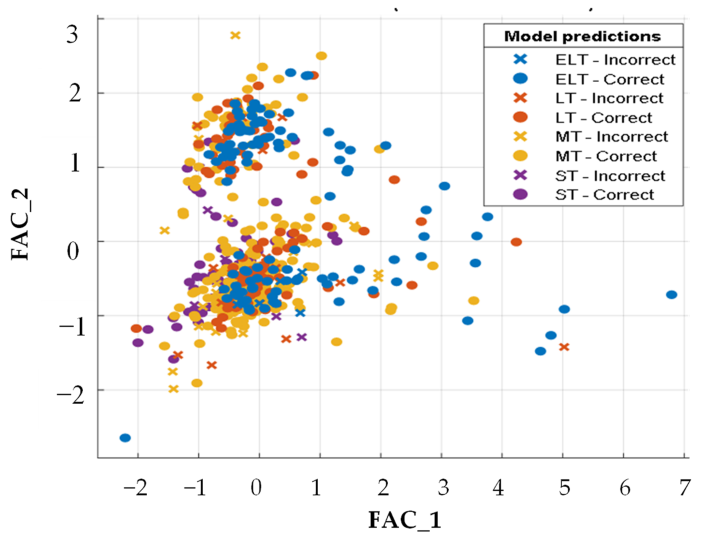
To understand how the selected classifier performed in each class, a confusion matrix plot was employed. True positive rates (TPRs) and false negative rates (FNRs) were used to determine how well the classifier performed in each class. The proportion of correctly identified observations per true class is referred to as the TPR. The FNR is the percentage of observations that are erroneously categorized in each class. Scattered plots are shown in Figure 9. Figure 10 reveals that 94.7%, 84.6%, 87.4%, and 72.9% of the extra-long trips (ELTs), long trips (LTs), medium trips (MTs), and short trips (STs), respectively, were correctly classified, as shown in the blue cells in the TPR column.

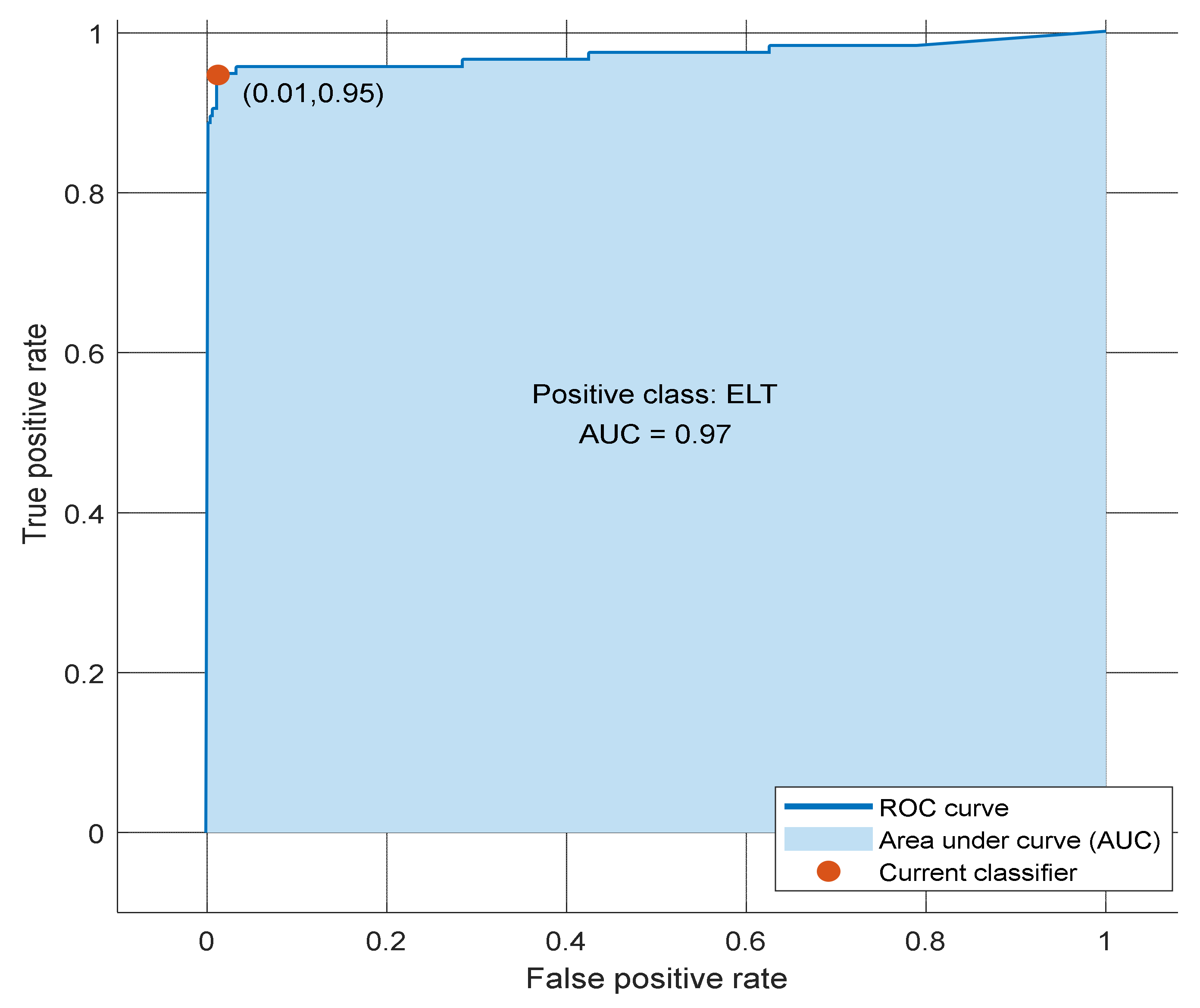
The receiver operating characteristic (ROC) curve in Figure 11 shows true and false positive rates for the NN-trained classifier. The false positive rate (FPR) of the selected method was 0.01, which indicates that the classifier assigns 1% of the observations incorrectly to the positive class. A TPR of 0.95 indicates that the classifier assigns 95% of the observations correctly to the positive class. The area under the curve is the measure of the overall quality of the classifier. The area under the curve of 0.97 indicates a better classifier performance.

3.1.3. NN Clustering Results Analysis

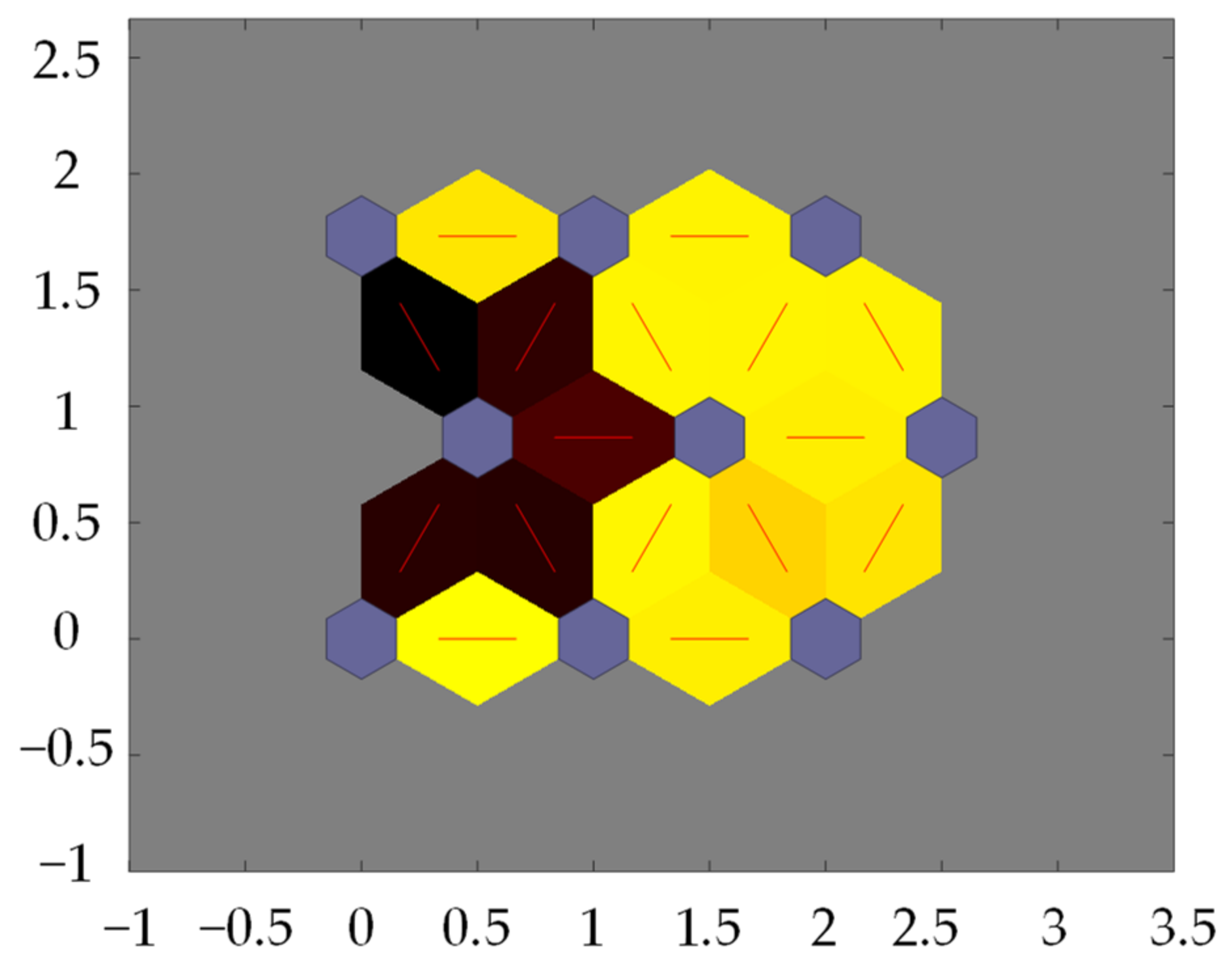
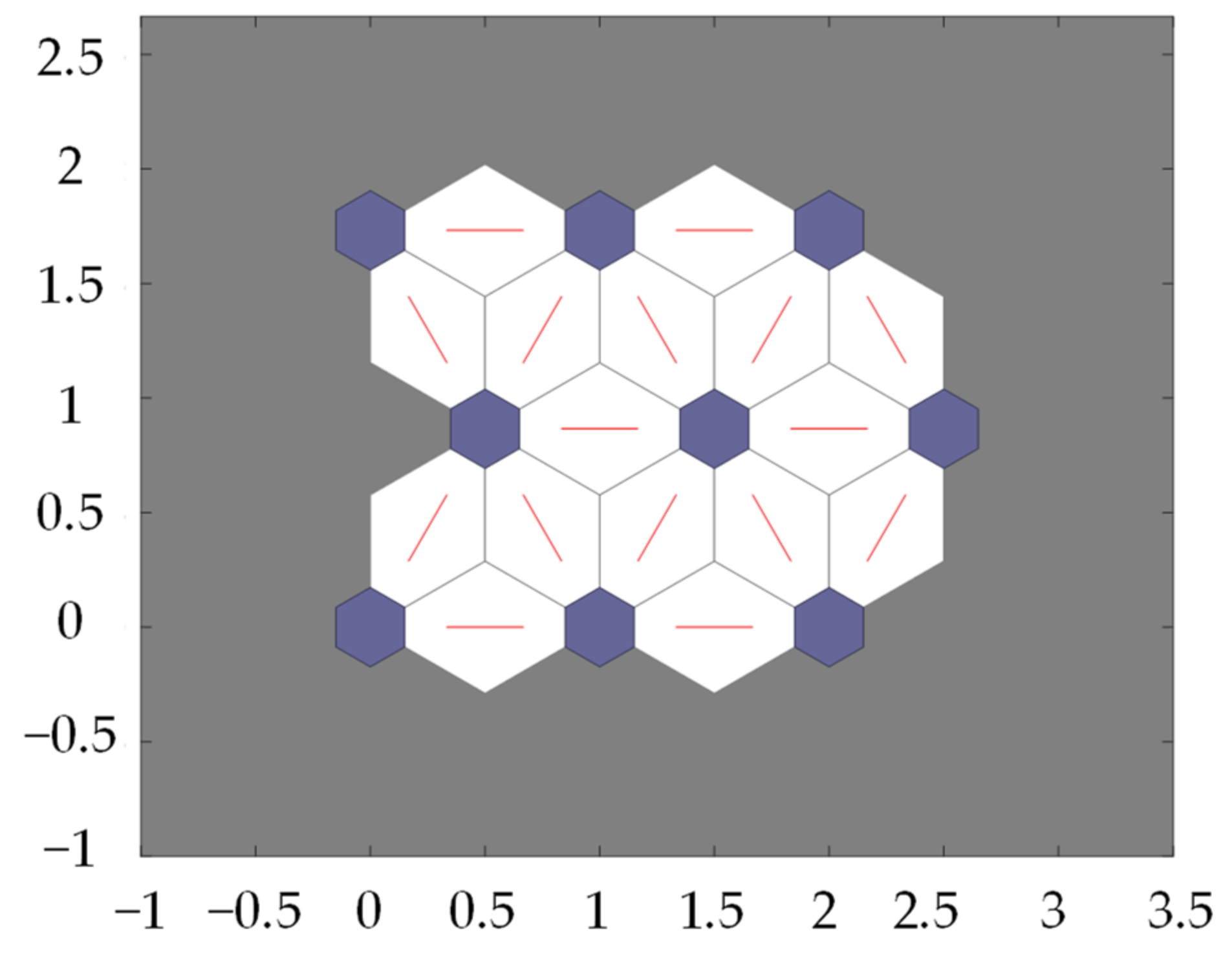
To cluster the five score values of PCA, a 3 × 3 matrix dimension was set for the number of classifications using the NN clustering algorithm. It categorized the 527 trips into nine groups. As shown in Figure 12, Figure 13 and Figure 14, the self-organizing map neighbor weight distances, neighbor connections, and weight positions indicated the best clustering performance. The Figure 12 uses the following color coding: the blue hexagons represent the neurons; the red lines connect neighboring neurons, the colors in the regions containing the red lines indicate the distances between neurons, the darker colors represent larger distances, and the lighter colors represent smaller distances. In Figure 13 SOM layer denotes neurons as gray-blue patches and its direct neighbor relations with red lines in SOM neighbor weight distances. Black to yellow color patches shows how close each neuron’s weight vector to its neighbors. In Figure 14 the button shows the locations of the data points and the weight vectors. In SOM weight positions, green dots denotes input vectors and shows how SOM classifies the input space by showing blue-gray dots for each neuron’s weight vector and connecting neighboring neurons with red lines represents the data on various clusters. Each cluster is shown in different colors. Gray-blue patches denote SOM layer neurons and red lines as their direct neighbor relations.

The number of trips in these nine categories was 77, 58, 75, 25, 31, 136, 15, 68, and 42 for clusters 1–9, respectively.

3.1.4. Selected Trips and Micro Trips

After computing the relative error and similarity score for each cluster, the trips that best represented their cluster were selected as the best trip. Based on this, nine best trips were selected. The similarity score of the nine best trips was 0.97, 0.95, 0.96, 0.87, 0.92, 0.98, 0.86, 0.99, and 0.98 for cluster numbers 1–9, respectively. However, the trip indicators were treated equally in the calculation.

The nine best trips selected were divided into MTs, and characteristic parameters were determined for each. The MTs that best represent their group were selected based on similarity scores. From the nine clusters, 18 MTs were chosen. As shown in

Table 6. Selected MTs.

Sequence Number	MT Code	Ttotal	Tidle	Tdrive	S	Route
1	EMT1	245	174	71	245.766	Urban
2	DMT7	229	107	122	430.225	Urban
3	CMT12	154	101	53	300.688	Urban
4	IMT8	119	45	74	332.236	Urban
5	EMT6	72	41	31	130.299	Urban
6	CMT2	82	37	45	281.14	Urban
7	HMT26	70	19	51	288.133	Urban
8	HMT10	72	19	53	240.567	Urban
9	FMT4	160	17	143	664.625	Urban
10	DMT11	50	10	40	79.368	Urban
11	FMT12	70	8	62	244.875	Urban
12	BMT6	51	7	44	183.937	Urban
13	AMTC29	90	35	55	434.186	Extra-urban
14	AMTC2	110	35	75	491.025	Extra-urban
15	BMT7	111	15	96	609.743	Extra-urban
16	GMT90	130	9	121	643.646	Extra-urban
17	IMT4	339	25	314	2098.639	Rural
18	GMT33	180	5	175	1210.502	Rural
19	RRMT3	160	3	157	1918.478	Ring road
20	EWMTC18	100	24	76	820.486	Expressway
Total		2594	736	1858	11,648.57

, sequence numbers 1–12, 13–16, and 17–18 represent selected MTs of urban, extra-urban, and rural road sections, respectively. Additionally, all ring road and expressway driving data were divided into MTs. One best MT was selected for the ring road section (sequence number 19 in Table 6), and one best MT was selected for the expressway section (sequence number 20 in Table 6).

3.1.5. NN-Based Speed Prediction

To predict a series of vehicle speeds y(t) for each route type based on a past value d of y(t) and another series of data x(t) using the NN, the nonlinear autoregressive with external input (NARX) model was applied. To train the network, Bayesian regularization and a back-propagation training algorithm were used. The best training performance was obtained at 177, 431, 554, 676, and 214 epochs for the urban, extra-urban, rural, ring road, and expressway sections, respectively. The response of the speed output element with training and test data is shown in Figure 15 for each route category.

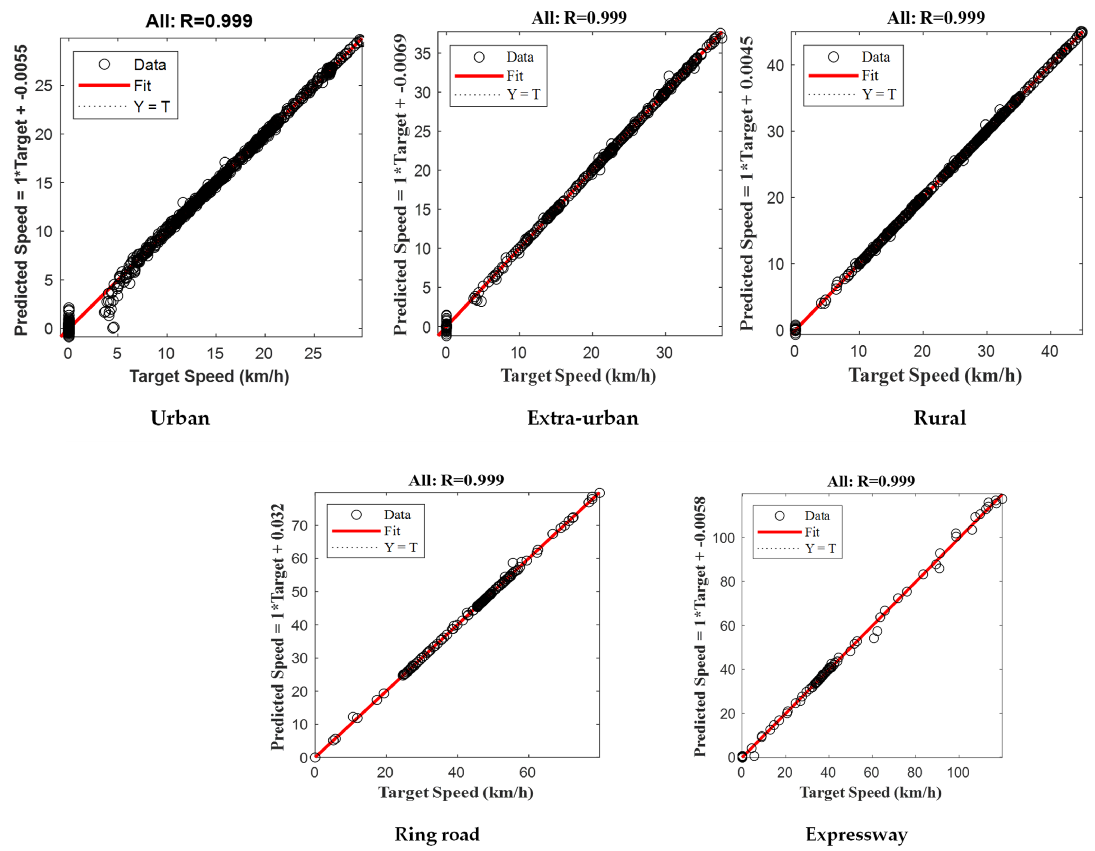
The regression fit of the training data, the test data, and all training and test data is shown in Figure 16. The regression fit of the training and test data is shown in Appendix A (Figure A1), as the R-value for each route was indicated to be greater than 0.99, which indicates the best fit. Therefore, the predicted value of speed for the given time series was used in the final AADC.

3.1.6. Developed Addis Ababa Driving Cycle (AADC)

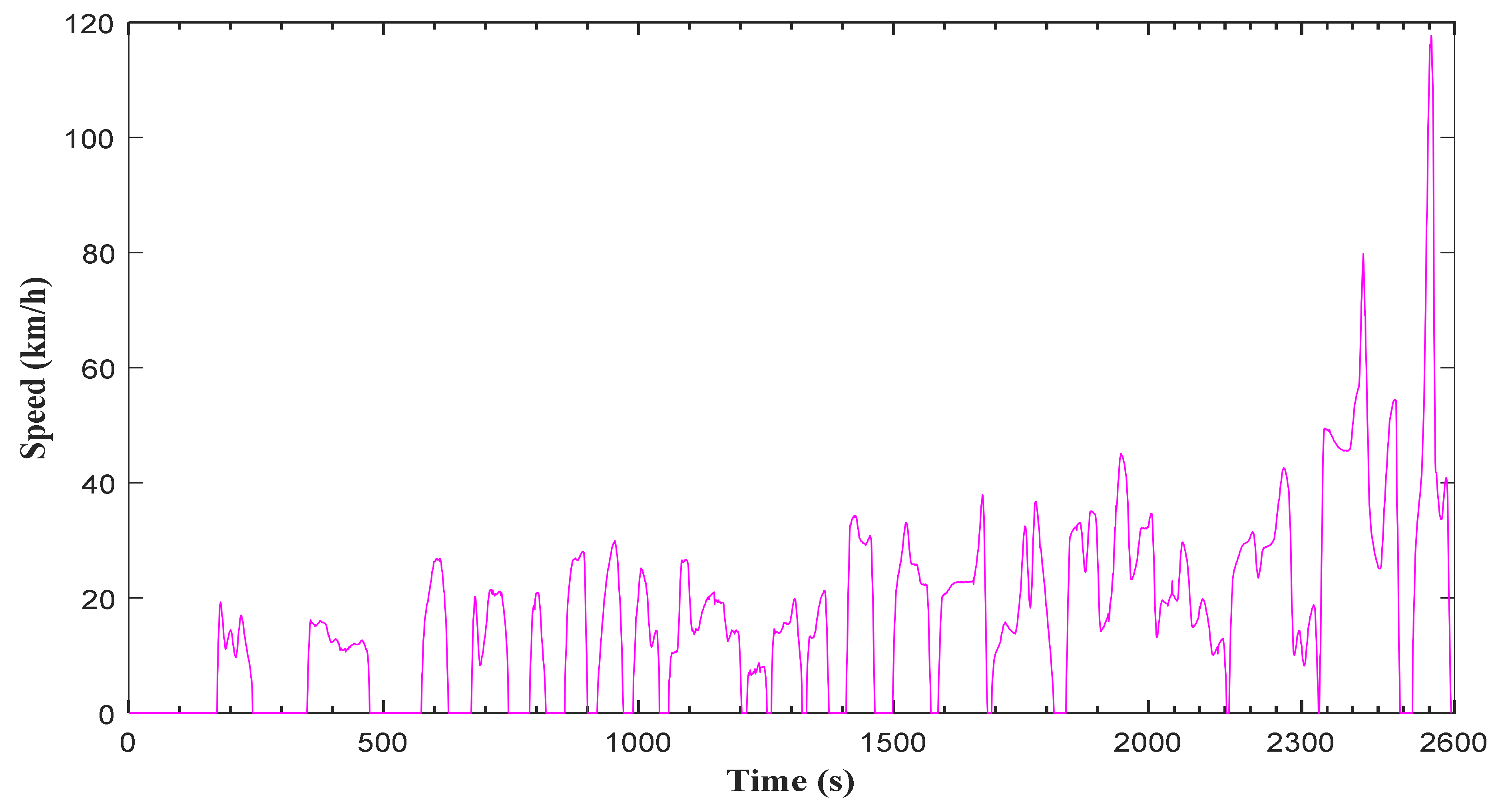
The DC developed was derived by combining the predicted vehicle velocity of the urban, extra-urban, rural, ring road, and expressway sections, as discussed in the section on NN-based prediction. The urban, extra-urban, rural, ring road, and expressway sections had durations of 1374 s, 441 s, 519 s, 160 s, and 100 s, respectively, as shown in

Table 7. AADC characteristic parameters of each route section.

Indicators	Urban	Extra-Urban	Rural	Ring Road	Expressway
Ssum	3400.659	2176.239	3306.434	1946.877	1055.271
Ttotal	1374	441	519	160	100
Vdavg	15.797	22.644	24.39	44.64	50.652
Vmax	29.847	37.919	45.10	79.762	117.67
Vsd	2.497	3.212	2.95	4.057	9.525
Vavg_all	8.91	17.766	22.936	43.805	38
decmax	−2.133	−1.824	−1.198	−3.584	−4.5
amax	1.975	1.876	2.147	2.705	3.44
asd	0.291	0.393	0.333	0.73	1.205
Nspkm	3.529	1.838	0.605	0.514	0.948
RPA	0.079	0.1	0.091	0.173	0.507
PKE	0.175	0.215	0.191	0.365	1.06
Pidl	0.436	0.215	0.06	0.019	0.25
Pacc	0.146	0.215	0.249	0.331	0.43
Pcru	0.272	0.37	0.451	0.45	0.05
Pdec	0.146	0.2	0.241	0.2	0.27

.

A final speed–time profile of the DC in Addis Ababa is shown in Figure 17 and its characteristic parameters are presented in Table 7. This is the transient DC, which consists of 20 MTs. The total duration of the DC was 2594 s, the distance covered was 11.885 km, and the average and maximum speed were 16.495 km/h and 117.67 km/h, respectively.

In this approach, a machine classification learner was applied to classify trips, and the NN clustering method was found to provide better performance accuracy than the other approaches. However, [6,7,10,13] applied the k-means clustering algorithm to the principal component score to classify the driving sequences into different clusters.

The DC duration was not determined on the basis of previous studies; rather, the methodology proposed in this study provided the DC duration that best matched the data collected in real time. Based on this method, a DC duration of 2594 s was obtained, and it had a deviation of 0.14 from the daily average trip duration, which indicates that the duration of this DC is close to the real-time driving data. However, [5] initially decided to apply a DC duration of between 1200 s and 1300 s, and two DCs were developed that have a duration of 1216 s and 1261 s. Peng et al. (2015) defined the duration of the designed DC as 1200 s [7]. Similarly, the authors of [6] decided on a DC duration of 1200 s, while the authors of [8] randomly constituted a DC until the required cycle duration was achieved. Additionally, the distance covered by this DC is 11.885 km with a relative difference of 0.13, which is close to the average daily trip distance of 13.667 km.

3.2. Micro Trip Method

The driving characteristic parameters reported in

Table 8. Composite characteristic parameters in each cluster.

Parameters	Cluster
	1	2	3	4	5	6
Number of MTs	104	1754	1438	593	1296	1495
Share of total duration	0.049	0.191	0.32	0.091	0.064	0.284
Vmax	120	40	50.2	80	9.2	30
Vavg	50.035	16.471	23.11	42.083	4.972	8.561
Vdavg	55.068	21.345	25.02	46.522	6.871	15.478
Accmax	3.556	2.066	2.384	2.919	1.106	1.868
Decmax	−4.399	−2.004	−1.238	−3.272	−1.278	−2.5
PAccavg	0.732	0.25	0.188	0.297	0.15	0.222
Decavg	−1.287	−0.273	−0.272	−0.394	−0.201	−0.261
Pacc	0.249	0.247	0.286	0.312	0.142	0.155
Pcru	0.464	0.285	0.309	0.333	0.388	0.239
Pdec	0.24	0.239	0.27	0.288	0.192	0.167
Pidl	0.097	0.228	0.136	0.067	0.278	0.439
Traffic condition/route	Expressway	Extra-urban	Rural	Ring road	Congested	Urban

were calculated after the speed time data were denoised and segmented into MTs using MATLAB. With the help of the K-means clustering algorithm, 6680 MTs were grouped into six clusters. As shown in Table 8 and Figure 18, the distributions of composite characteristic parameters in clusters 1, 2, 3, 4, 5, and 6 are considered to be expressway, extra-urban, rural, ring road, congested (urban low-speed phase), and urban (medium-speed phase) conditions, respectively. There are 1296, 1495, 1754, 1438, 593, and 104 micro trips in the congested, urban, extra-urban, rural, ring road, and expressway sections, respectively.

Using this MT approach, we produced different candidate DCs. From among them, we selected the best one that has the least paired CPs. Its characteristic parameters are shown in

Table 9. Characteristic parameters of the candidate DC based on route analysis.

CPs	Vmax	Vavg	Vdavg	Accmax	Decmax	PAccavg	Decavg	Pacc	Pcru	Pdec	Pidl
Urban	30	8.102	14.178	1.3279	−1.4	0.194	−0.251	0.16	0.242	0.17	0.428
Extra-urban	40	16.25	21.408	1.776	−1.662	0.25	−0.277	0.22	0.341	0.194	0.241
Rural	51.8	22.008	25.47	1.2526	−1.332	0.263	−0.263	0.26	0.325	0.279	0.136
Ring road	69.1	42.285	45.44	2.8559	−2.749	0.345	−0.465	0.39	0.306	0.236	0.069
Expressway	109	59.222	64.552	3.0556	−4.469	0.601	−0.786	0.36	0.303	0.257	0.082
Overall DC	109	20.426	27.287	3.0556	−4.469	0.281	−0.325	0.24	0.293	0.218	0.252

, and the candidate DC developed using the MT method is shown in Figure 19. The total time (Ttotal) of this cycle is 1539 s, of which the urban, extra-urban, rural, ring road, and expressway sections covered 553, 299, 434, 144, and 109 s, respectively. The total distance of the cycle is 8.73 km, of which the urban, extra-urban, rural, ring road, and expressway sections covered 1.24, 1.35, 2.65, 1.69, and 1.79 km, respectively. The DC developed using the MT method contains a total of 10 MTs (including 2 MTs in the congested section, 3 MTs in the urban section, 2 MTs in the extra-urban section, 1 MT in the rural section, 1 MT in the ring road section, and 1 MT in the expressway section) with a total duration of 1539 s and a distance of 8.732 km. Figure 19 depicts the candidate cycle’s speed profile, which includes the cycle’s top speed of 109 km/h, overall average speed of 20.426 km/h, driving average speed of 27.287 km/h, and idle ratio of 0.252.

4. Discussion

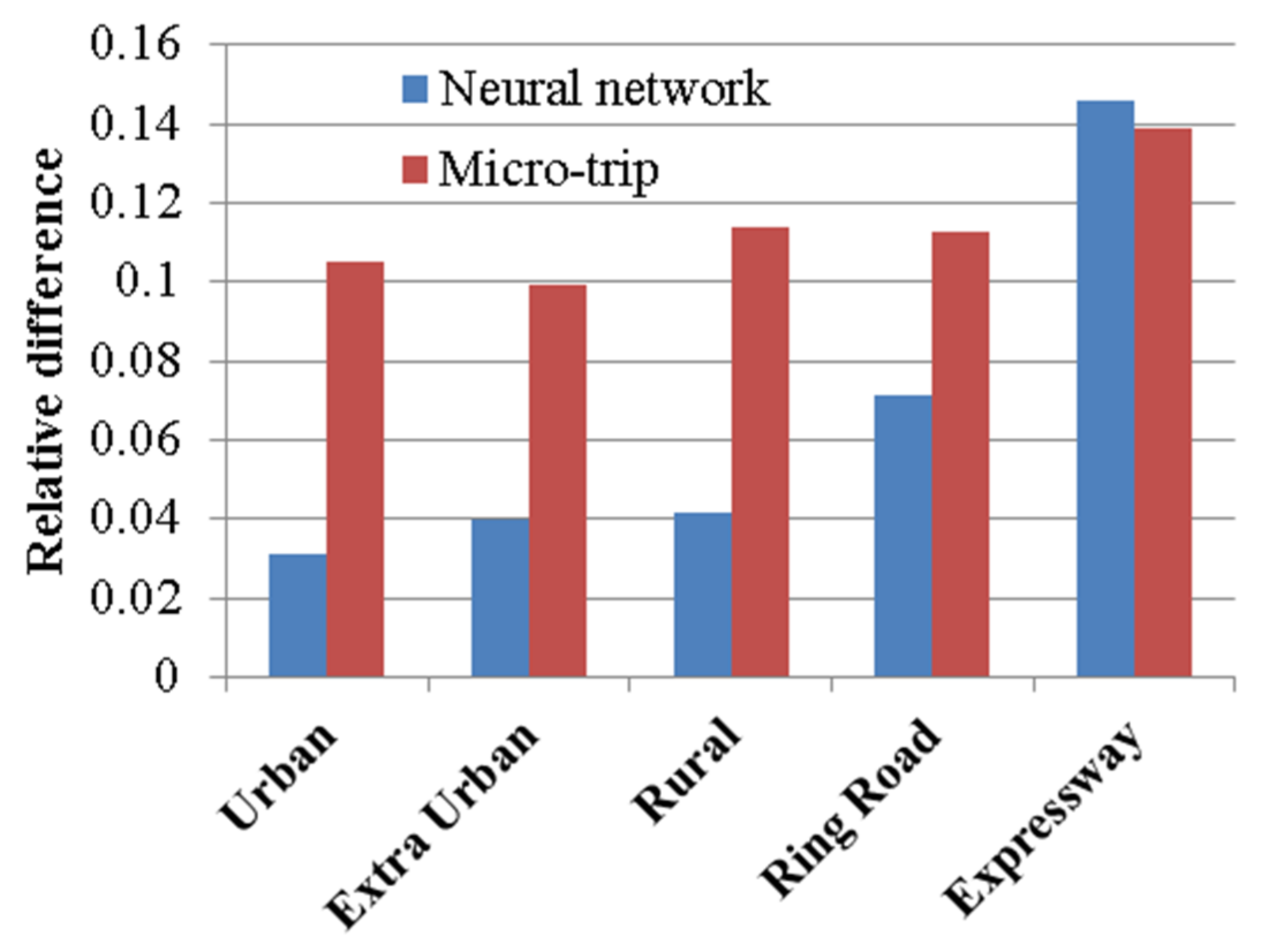
Following the application of the two approaches described above, we determined each method’s corresponding DC and evaluated how well the DCs corresponded to the driving circumstances in Addis Ababa. The values obtained for the paired CPs of each route compared to the target are given in Figure 20. We used all of the CPs provided in Table 9 to evaluate the representativeness of the developed DCs. With regard to the urban, extra-urban, rural, ring road, and expressway sections, the applied NN method represents 96.91%, 96%, 95.81%, 92.85%, and 85.3%, respectively, compared with the target data. However, the MT method represented 89.48%, 90.1%, 88.6%, 88.73%, and 86.1% of the urban, extra-urban, rural, ring road, and expressway sections, respectively. This result indicates that the NN method improved the degree of representativeness by 7.43%, 5.9%, 7.21%, and 4.11% for the urban, extra-urban, rural, and ring road sections, respectively. For the NN prediction method, the resulting DC precisely depicts all the CPs that describes each route compared with the MT method except for the expressway section. Due to the expressway’s extended travel distances without stops, we noticed that the paired CPs for the NN method are quite close to the maximum established deviation. Additionally, compared with the training data for the other routes, fewer data were used to train the NN on the expressway.

The duration characteristics of DCs developed using the NN prediction and MT methods were compared. From the comparison of duration characteristics, the DC developed by the NN method is longer (2594 s), while the DC developed using the MT method is relatively short (1539 s). The DC duration obtained using NN prediction is very close to the daily trip average duration of 3051 s. The distance of the DC obtained using NN-based prediction is longer (11.885 km), and the MT-based cycle distance is shorter (8.732 km). However, the daily average trip distance of the collected data is 13.667 km, which is very close to the distance of the DC obtained using NN prediction with a relative difference of 0.13.

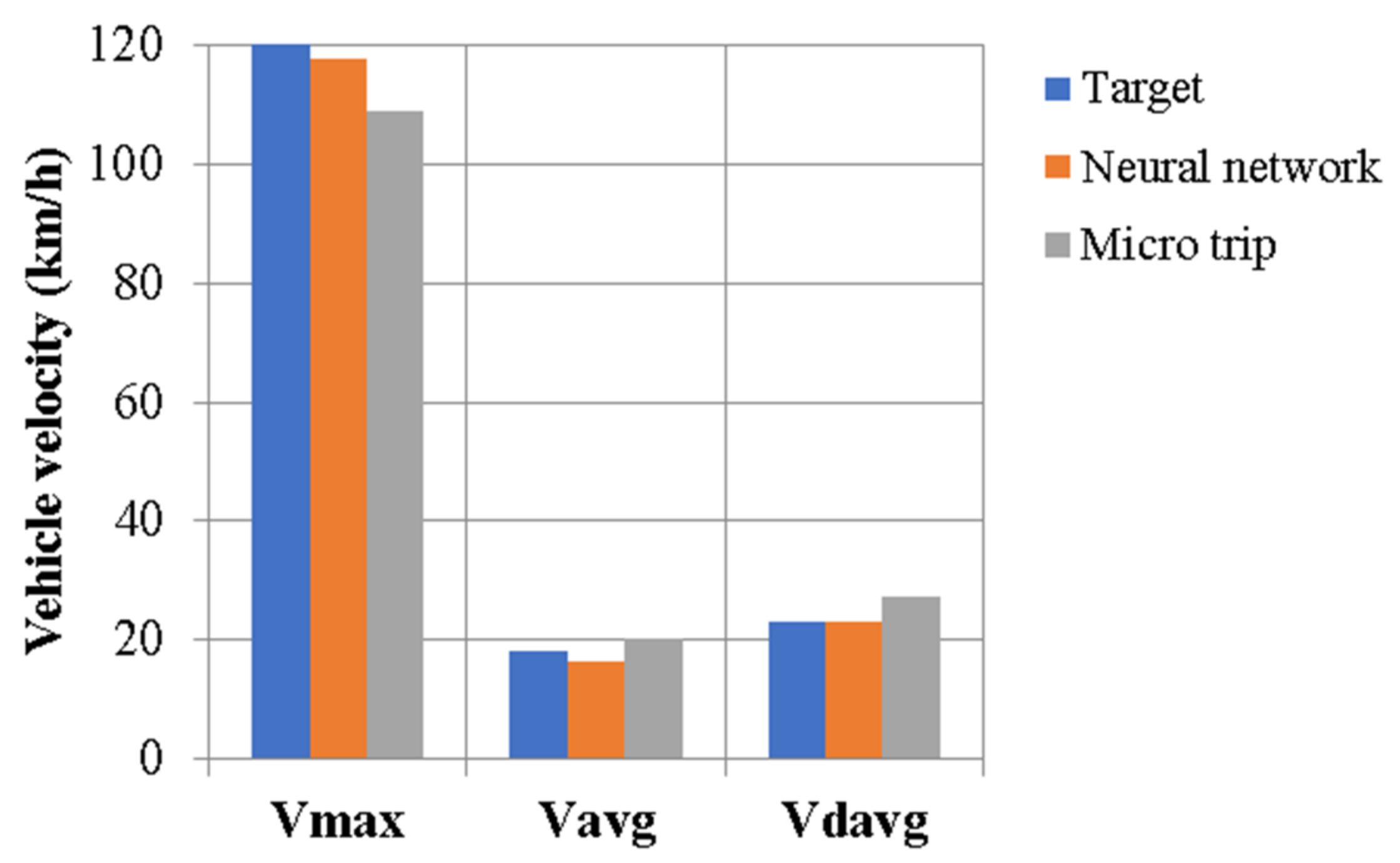
Figure 21 shows the comparison of vehicle velocity characteristics of the processed experimental data and the DCs developed using the two methods. From the perspective of the maximum velocity, average velocity, and average driving velocity, the NN method is the closest to the target compared with the MT method. This means that the speed distribution of the NN method is consistent and representative of the actual driving conditions of Addis Ababa city.

From the point of view of the maximum acceleration and deceleration, the NN-based DC has a relative deviation of 0.005 and 0.023 and the MT method has a relative deviation of 0.116 and 0.016 from the target, respectively. From the comparison of the average acceleration and deceleration, it was found that the NN-based DC is closest to the target data compared with the MT-based DC. Additionally, the values of the acceleration-related parameters of the DC developed using the NN are higher than those of the MT-based cycle, indicating that the acceleration and deceleration processes are more aggressive than the MT method.

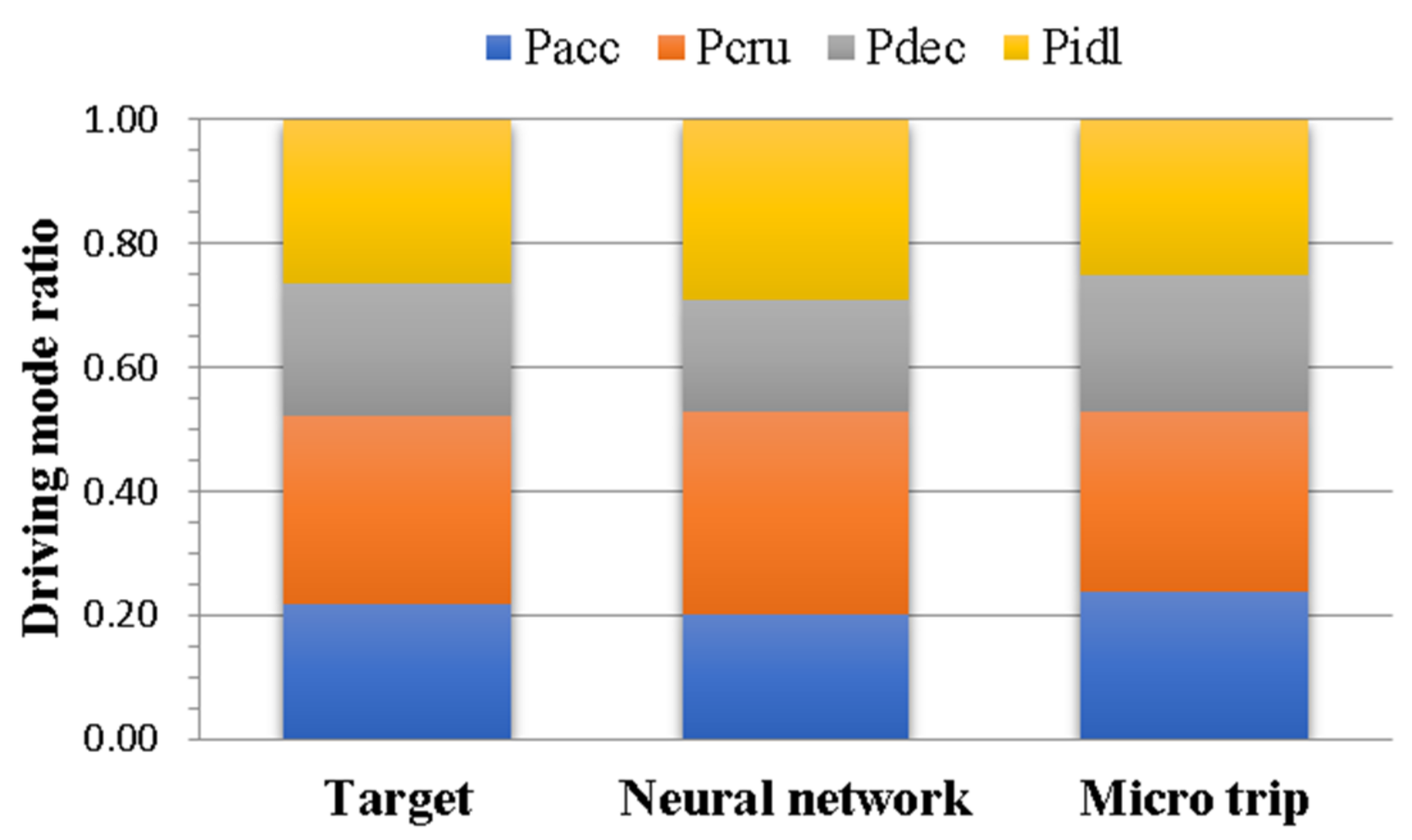
From the distribution of the driving mode ratio of the idle, acceleration, deceleration, and cruising times, the driving modes of the developed DCs are very close to the processed experimental data as shown in Figure 22. However, the deviation of the driving modes of the MT-based cycle is smaller than that of the NN method.

The DC developed using NN prediction is closer to the results of the processed experimental data compared with the DC developed using the MT method in terms of all characteristic parameters. We also found that all CPs of the DC developed using the MT method were within the threshold except for the average deceleration (Decavg). As shown in

Table 10. The relative difference in CPs between the target and developed DCs.

CPi	Target	NN		MT
		AADC	RDi	DC	RDi
Vmax	120	117.67	0.019	109	0.092
Vavg	18.064	16.495	0.087	21.247	0.131
Vdavg	23.241	23.242	0.001	27.476	0.141
Accmax	3.456	3.44	0.005	3.056	0.116
Decmax	−4.399	−4.5	0.023	−4.469	0.016
PAccavg	0.338	0.355	0.05	0.304	0.15
Decavg	−0.491	−0.47	0.043	−0.398	0.338
Pacc	0.218	0.2	0.084	0.236	0.083
Pcru	0.303	0.327	0.078	0.295	0.033
Pdec	0.214	0.182	0.128	0.218	0.018
Pidl	0.264	0.29	0.099	0.251	0.045
RD			0.056		0.111

, the DC developed using NN prediction has smaller deviations than the DC developed using the MT method, which has a relative difference (RD) of 0.056 and 0.111, respectively. This indicates that the cycle developed using the NN improved the degree of representativeness by 5.5% compared with the MT method.

The NN prediction method proposed in this study, as the result demonstrates, considerably enhances the whole cycle’s representativeness by 5.5% and resolves the issue with the DC duration decision and the lower degree of representativeness of the MT method. The following factors contributed to the results: the trip method proposed in this study is the foundation for the determination of the DC duration, applying machine learning classification for clustering, and, after being processed, the collected driving data were used to train an NN, which then predicted the velocity of the DC. Therefore, the DC developed in this study using the NN method accurately represents the driving conditions in Addis Ababa.

Comparison of AADC with Standard DCs

Compared with existing standard DCs, the AADC has the capacity to describe actual traffic conditions on Addis Ababa’s roads most accurately. A comparison of characteristic indicators from the FTP-75, WLTC, CLTC, collected data, and final DC developed in this study (AADC) was performed (

Table 11. Comparison of the developed AADC with standard DCs.

CPi	Target	AADC	RDi	WLTC	RDi	FTP-75	RDi	CLTC	RDi
Vmax	120	117.67	0.019	131.31	0.094	91.25	0.240	114	0.050
Vavg	18.064	16.495	0.087	46.5	1.574	33.89	0.876	28.96	0.603
Vdavg	23.241	23.242	0.001	53.15	1.287	25.82	0.111	37.15	0.599
Accmax	3.456	3.44	0.005	1.75	0.494	1.48	0.572	1.47	0.575
Decmax	−4.399	−4.5	0.023	−1.5	0.659	−1.48	0.664	−1.47	0.666
PAccavg	0.338	0.355	0.05	0.42	0.243	0.51	0.509	0.45	0.331
Decavg	−0.491	−0.47	0.043	−0.44	0.104	−0.58	0.181	−0.49	0.002
Pacc	0.218	0.2	0.084	0.309	0.417	0.311	0.427	0.286	0.312
Pcru	0.303	0.327	0.078	0.278	0.083	0.247	0.185	0.228	0.248
Pdec	0.214	0.182	0.128	0.286	0.336	0.271	0.266	0.264	0.234
Pidl	0.264	0.29	0.099	0.127	0.519	0.172	0.348	0.221	0.163
RD			0.056		0.528		0.398		0.344

). The results show that the method proposed in this study solved the problem of determining the DC duration. The relative difference of the AADC, WLTC, FTP-75, and CLTC was −0.056, 0.528, 0.398, and 0.344, respectively. This indicates that, compared with existing DCs in other countries, the AADC developed here better suits the actual road and traffic conditions in Addis Ababa in terms of all characteristic parameters used in this study. Additionally, the characteristic parameters of the developed AADC are closer to the data sources and are thus representative.

When looking at acceleration-related indicators, the driving characteristics for the AADC were quite different from those of standard DCs. The cycles developed in this study exhibited significantly higher acceleration and deceleration rates as well as much longer idling periods than standard DCs. The frequent vehicle stops and movements due to traffic congestion and closer traffic light signals revealed long idling periods in the AADC. The developed AADC has a relatively long duration (2594 s) but a shorter trip length (11.885 km) compared with the WLTC, FTP-75, and CLTC.

5. Conclusions

The analysis of real-time driving data collected from passenger vehicles in Addis Ababa using GPS devices revealed that standard DCs deviate considerably from the actual conditions, and therefore an Addis Ababa DC should be developed and used for the evaluation of vehicle emissions and fuel consumption.

In this study, a trip-based approach combining principal component analysis and neural network prediction was proposed in order to construct a representative DC and compared with the micro trip approach to DC development in order to solve the issue of having to determine DC duration based on experience and the literature. The collected data were divided into 726 trips. Using eigenvalue decomposition, principal component analysis reduced the 17 trip indicators to five principal components. The machine classification learner results indicate that the neural network classifier had an accuracy of between 82.9% and 86.5%. The applied neural network algorithm classified 527 trips into nine clusters based on the factor scoring of each trip.

After training the neural network, the Addis Ababa DC speed was predicted with an overall R-value of 0.99, indicating the best fit between the input and target parameters. The comparative analysis of the neural network and micro trip methods with processed experimental data showed a relative difference of 0.056 and 0.111, respectively. Additionally, compared with the daily average trip length, the DC duration and distance obtained using the neural-network-based method show the smallest deviations of 0.14 and 0.13, respectively. The results of the comparison show that the DC created using the neural-network-based method more accurately represents the actual driving conditions in Addis Ababa compared with the micro trip method due to the application of the trip approach, machine learning classification, and neural-network-based speed prediction. Additionally, compared with standard DCs, it reflects the actual driving conditions more closely than WLTC, FTP-75, and CLTC. Consequently, the developed AADC can also be used for the evaluation of the emissions and fuel consumption of vehicles in Addis Ababa. We strongly suggest that the administration of Addis Ababa make the AADC the legislative driving cycle of the city. Future studies on DCs could test the proposed methodology using bulk driving data and apply weightings to trip indicators.

References

1. Teoh, J.X.; Stella, M.; Chew, K.W. Performance Analysis of Electric Vehicle in Worldwide Harmonized Light Vehicles Test Procedure via Vehicle Simulation Models in ADVISOR. In Proceedings of the International Conference on System Engineering and Technology (ICSET), Shah Alam, Malaysia, 7 October 2019; Volume 9, pp. 215–220. [Google Scholar]
2. Gebisa, A.; Gebresenbet, G.; Gopal, R.; Nallamothu, R.B. Driving Cycles for Estimating Vehicle Emission Levels and Energy Consumption. Future Transp. 2021, 1, 615–638. [Google Scholar] [CrossRef]
3. Tsanakas, N.; Ekström, J.; Olstam, J. Estimating Emissions from Static Traffic Models: Problems and Solutions. J. Adv. Transp. 2020, 2020, 5401792. [Google Scholar] [CrossRef] [Green Version]
4. Liu, Y.; Liang, Y.; Yu, H.; An, X.; Li, J. Comparative Analysis of China Light-duty Vehicle Test cycle for Passenger Car and Other Typical Driving Cycles. E3S Web Conf. 2021, 241, 02002. [Google Scholar] [CrossRef]
5. Zhao, M.; Gao, H.; Han, Q.; Ge, J.; Wang, W.; Qu, J. Development of a Driving Cycle for Fuzhou Using K-Means and AMPSO. J. Adv. Transp. 2021, 2021, 5430137. [Google Scholar] [CrossRef]
6. Guo, S.; Wu, K.; Zhang, G. Application of PCA-K-means++ combination model to construction of light vehicle driving conditions in intelligent traffic. J. Meas. Eng. 2020, 8, 107–121. [Google Scholar] [CrossRef]
7. Peng, J.; Pan, D.; He, H. Study on the driving cycle construction for city hybrid bus. In Proceedings of the International Conference on Intelligent Systems Research and Mechatronics Engineering (ISRME 2015), Zhengzhou, China, 11–13 April 2015; pp. 1491–1497. [Google Scholar]
8. Tong, H.Y.; Ng, K.W. A bottom-up clustering approach to identify bus driving patterns and to develop bus driving cycles for Hong Kong. Environ. Sci. Pollut. Res. 2020, 28, 14343–14357. [Google Scholar] [CrossRef] [PubMed]
9. Liu, H.; Zhao, J.; Qing, T.; Li, X.; Wang, Z. Energy consumption analysis of a parallel PHEV with different configurations based on a typical driving cycle. Energy Rep. 2021, 7, 254–265. [Google Scholar] [CrossRef]
10. Ji, Y.; Li, C.; Xie, J.; Wang, Y.; Guo, W. Bus Driving Cycle Construct Based on Principal Component Analysis for Lanzhou City. In Proceedings of the 14th International Conference on Wireless Communications, Networking and Mobile Computing (WiCOM 2018), Limassol, Cyprus, 15–17 October 2018; pp. 416–425. [Google Scholar]
11. Liu, X.; Ma, J.; Zhao, X.; Du, J.; Xiong, Y. Study on Driving Cycle Synthesis Method for City Buses considering Random Passenger Load. J. Adv. Transp. 2020, 2020, 3871703. [Google Scholar] [CrossRef]
12. Peng, Y.; Zhuang, Y.; Yang, Y. A driving cycle construction methodology combining k-means clustering and Markov model for urban mixed roads. Automob. Eng. 2019, 234, 714–724. [Google Scholar] [CrossRef]
13. Zhou, W.; Xu, K.; Yang, Y.; Lu, J. Driving Cycle Development for Electric Vehicle Application Using Principal Component Analysis and K-means Cluster: With the Case of Shenyang, China. In Proceedings of the 8th International Conference on Applied Energy, ICAE2016, Beijing, China, 8–11 October 2016; Volume 105, pp. 2831–2836. [Google Scholar] [CrossRef]
14. Wu, Y.; Zhang, W.; Zhang, L.; Qiao, Y.; Yang, J.; Cheng, C. A Multi-Clustering Algorithm to Solve Driving Cycle Prediction Problems Based on Unbalanced Data Sets: A Chinese Case Study. Sensors 2020, 20, 2448. [Google Scholar] [CrossRef] [PubMed]
15. Chen, Z.; Yang, C.; Fang, S. A Convolutional Neural Network-Based Driving Cycle Prediction Method for Plug-in Hybrid Electric Vehicles With Bus Route. IEEE Access 2020, 8, 3255–3264. [Google Scholar] [CrossRef]
16. Qiu, D.; Li, Y.; Qiao, D. Recurrent Neural Network Based Driving Cycle Development for Light Duty Vehicles in Beijing. Transp. Res. Procedia 2018, 34, 147–154. [Google Scholar] [CrossRef]
17. Zhao, P.; Wang, Y.; Chang, N.; Zhu, Q.; Lin, X. A Deep Reinforcement Learning Framework for Optimizing Fuel Economy of Hybrid Electric Vehicles. In Proceedings of the 2018 23rd Asia and South Pacific Design Automation Conference (ASP-DAC), Jeju, Korea, 22–25 January 2018; pp. 196–202. [Google Scholar]
18. World Population Review. Available online: http://worldpopulationreview.com/world-cities/addis-ababa-population/ (accessed on 25 September 2021).
19. Busho, S.W.; Alemayehu, D. Applying 3D-eco routing model to reduce environmental footprint of road transports in Addis Ababa City. Environ. Syst. Res. 2020, 9, 17. [Google Scholar] [CrossRef]
20. Baskin, A. Africa Used Vehicle Report. In Proceedings of the Africa Clean Mobility Week, Nairobi, Kenya, 12–16 March 2018. [Google Scholar]
21. Fekadu, Y. Contribution of Vehicle Exhausts Gas Emissions to the Traffic Air Pollution of Selected Areas of Addis Ababa City. Master’s Thesis, Addis Ababa University, Addis Ababa, Ethiopia, 2017. [Google Scholar]
22. Bikis, A.; Pandey, D. Air Quality at Public Transportation Stations/Stops: Contribution of Light Rail Transit to Reduce Air Pollution. Aerosol Sci. Eng. 2021, 6, 1–16. [Google Scholar] [CrossRef]
23. Liu, Y.; Li, J.; Shen, B. Research on Driving Cycle of Long-distance Passenger Vehicles Based on Principal Component Analysis and Cluster Algorithm. Int. J. Control Autom. 2014, 7, 125–136. [Google Scholar] [CrossRef]
24. George, B. Extensions of the General Linear Model into Methods within Partial Least Squares Structural Equation Modeling; University of North Texas: Denton, TX, USA, 2016. [Google Scholar]
25. Wang, Q.N.; Zeng, X.H.; Wang, P.Y.; Wang, J.N. Driving Cycle Recognition Neural Network Algorithm Based on the Sliding Time Window for Hybrid Electric Vehicles. Int. J. Automot. Technol. 2015, 16, 685–695. [Google Scholar] [CrossRef]
26. Xu, S. LVQ Neural Network based Driving Cycles Recognition for Hybrid Electric Vehicles. Appl. Mech. Mater. 2013, 253–255, 2113–2116. [Google Scholar] [CrossRef]
27. Huertas, J.I.; Quirama, L.F.; Giraldo, M.D.; Diaz, J. Comparison of driving cycles obtained by the Micro-trips, Markov-chains and MWD-CP methods. Int. J. Sustain. Energy Plan. Manag. 2019, 22, 109–120. [Google Scholar] [CrossRef]
28. Mahayadin, A.R.; Ibrahim, I.; Zunaidi, I.; Shahriman, A.B.; Faizi, M.K.; Sahari, M.; Hashim, M.S.M.; Saad, M.A.M.; Sarip, M.S.; Razlan, Z.M.; et al. Development of Driving Cycle Construction Methodology in Malaysia’s Urban Road System. In Proceedings of the 2018 International Conference on Computational Approach in Smart Systems Design and Applications (ICASSDA), Kuching, Malaysia, 15–17 August 2018; pp. 1–5. [Google Scholar] [CrossRef]
29. Arun, N.; Mahesh, S.; Ramadurai, G.; Nagendra, S.S. Development of driving cycles for passenger cars and motorcycles in Chennai, India. Sustain. Cities Soc. 2017, 32, 508–512. [Google Scholar] [CrossRef]
Figure 1. Study area map and live traffic on Addis Ababa’s main roads to different cities.
Sustainability 14 13772 g001
Figure 2. Percentage of distance traveled on each route type.
Sustainability 14 13772 g002
Figure 3. Framework of the proposed method.
Sustainability 14 13772 g003
Figure 4. Speed, acceleration, and slope distribution.
Sustainability 14 13772 g004
Figure 5. Speed vs. time of a sample trip.
Sustainability 14 13772 g005
Figure 6. Neural network clustering diagram.
Sustainability 14 13772 g006
Figure 7. Neural network diagram.
Sustainability 14 13772 g007
Figure 8. Scree plot.
Sustainability 14 13772 g008
Figure 9. Scattered plot of narrow NN.
Sustainability 14 13772 g009
Figure 10. Validation confusion matrix of the NN classifier.
Sustainability 14 13772 g010
Figure 11. ROC curve of the NN classifier.
Sustainability 14 13772 g011
Figure 12. Self-organizing map neighbor weight distances.
Sustainability 14 13772 g012
Figure 13. Self-organizing map neighbor connections.
Sustainability 14 13772 g013
Figure 14. Self-organizing map weight positions.
Sustainability 14 13772 g014
Figure 15. Response of the time series to the predicted vehicle speed.
Sustainability 14 13772 g015
Figure 16. Regression fit of all training and test data.
Sustainability 14 13772 g016
Figure 17. Developed AADC.
Sustainability 14 13772 g017
Figure 18. Clustering of MTs in the two-dimensional feature space.
Sustainability 14 13772 g018
Figure 19. Candidate DC developed using the MT method.
Sustainability 14 13772 g019
Figure 20. Route-based relative difference in paired CPs compared with the target.
Sustainability 14 13772 g020
Figure 21. Comparison of vehicle velocity characteristics.
Sustainability 14 13772 g021
Figure 22. Comparison of driving mode characteristics.
Sustainability 14 13772 g022