Article

Optimization of Snowplow Routes for Real-World Conditions

1
Department of Automotive and Mechatronics Engineering, Ontario Tech University, 2000 Simcoe Street North, Oshawa, ON L1G 0C5, Canada
2
Department of Civil and Environmental Engineering, University of Alberta, 116 St. & 85 Ave., Edmonton, AB T6G 2R3, Canada
3
Office of the Chief Administrative Officer, Municipality of Clarington, 40 Temperance Street, Bowmanville, ON L1C 3A6, Canada
*
Author to whom correspondence should be addressed.
Sustainability 2022, 14(20), 13130; https://doi.org/10.3390/su142013130
Submission received: 29 July 2022 / Revised: 8 October 2022 / Accepted: 8 October 2022 / Published: 13 October 2022

Abstract

:
During the winter season, snowplowing has a significant effect on road users as it is critical to winter road maintenance and operations. The main goal of this study is to generate optimal routes for snowplowing trucks for efficient road maintenance. In addition to the conventional problem of reducing travel time and distance, this study also incorporates actual operational constraints, such as minimum maintenance standards and driver safety, to improve the overall efficiency of operations. To achieve the objectives, we first implemented the Chinese Postman Problem (CPP) to create Euler circuits from the initial routes and then identified the shortest paths by applying Dijkstra’s algorithm. Then, the Tabu search algorithm was chosen as a metaheuristic algorithm for the optimization process that finds near-optimal solutions by considering operational constraints for snowplow routes. Unsafe turning conditions and minimum maintenance standards were taken into account in the objective function defined for the optimization process. In simulations, the route obtained by our approach was compared to one with the application of CPP only in terms of travel distance, time, turning conditions, and road maintenance priority.

1. Introduction

In Canada, snowplowing is one of the critical services provided by municipalities since snow accumulation on roads reduces surface traction and increases the chances of slippery conditions, which result in serious safety concerns.
Specifically, a slight delay in the snowplowing schedule can lead to thick sheets of ice that worsen the safety of drivers. In extreme cases, blockage of the storm drains for melting snow and ice may cause transportation to halt. Moreover, traffic flow can be reduced to around 40 percent of the free-flow speed on highways due to heavy snowfall [1], and traffic accidents can increase by up to 75 percent in the worst cases [2].
Optimizing the snowplow route plays a vital role in urban planning and sustainability. Optimizing snow plowing routes can facilitate quick and efficient snow removal operations that can reduce traffic delays, especially during rush hours. It also can contribute to reducing the operational time required to clear snow and to attenuating the risk of vehicles drifting off the road, potentially reducing accidents. Moreover, optimal routing improves the environmental sustainability of municipalities by reducing fuel consumption and carbon footprint.
One of the most promising approaches for improving snowplowing service efficiency and reducing costs is to identify optimal routes for snowplow trucks. However, snowplowing is a complex process due to multiple factors that have a direct impact on formulating such optimal routes. These factors include fuel consumption, unsafe maneuvers, and completion time [3] as operational constraints that need to be minimized in order to optimize snowplow routes.
Methodologically, the snowplow route optimization problem is similar to the Chinese Postman Problem (CPP) where every edge has to be serviced exactly once while minimizing the total distance traveled [3]. For this reason, the CPP can provide a good starting point to the route optimization that can be further refined with the help of an additional approach such as a heuristic algorithm to consider operational constraints. The snowplow route optimization problem is considered a combinatorial optimization problem as it seeks to find an optimal solution from a finite set of objects (i.e., a list of nodes) that generates a path to cover them in the shortest time while satisfying the constraints [4].
To deal with this combinatorial problem, optimization algorithms play an important role in designing efficient and optimal routes for snowplowing [3,5]. Malandraki et al. [6] proposed the idea of Maximum Benefit CPP (MBCPP) for the directed graphs. MBCPP relaxed the constraint required by the conventional CPP method, which transverses each edge at least once. In fact, each edge is associated with a service cost for traversal and a deadhead cost for traversal with no service. The objective of this study is to find a tour starting from a depot location and traversing a selected set of edges. Perrier et al. [7] developed a method of optimization based on the hierarchy of the roads. In the study, the high-priority roads were plowed first followed by the lower priorities, which helps meet the road class (priority) requirements.
Kinable et al. analyzed the performance of three different optimization models: mixed-integer programming, constraint programming, and constructive heuristic procedure. The presented models were designed to consider both plowing and salt-spreading operations [8]. Sullivan et al. proposed an iterative method to deal with the vehicle allocation and ice control system. In this study, a heuristic approach was applied to the clusters in the network for reallocating vehicles to achieve more effective ice and snow control than simply increasing the fleet size [9].
Codur et al. [10] proposed a time-dependent variant of the Hierarchical Chinese Postman Problem (HCCP). Through mixed-integer linear programming, the proposed method minimizes the total travel time while maintaining precedence relationships between edges. The study of Korteweg et al. [11] also presented a method of improving the HCCP by considering the lexicographic criterion which minimizes priority class costs. Ahabchane et al. [12] addressed the issue of road salt spreading during the winter season by presenting a variant of the Slack Induction by String Removals (SISRs) metaheuristic. In this study, an optimization method for the road priority hierarchy was developed by formulating the mixed capacitated general routing problem with demand variation due to traffic or weather conditions.
In the domain of path planning, ref. [13] applied a multi-objective optimization technique to minimize the total distance and collision avoidance where the primary cost and second functions are minimized for path length and collision avoidance, respectively. Most snowplow routing problems, however, focus on reducing travel distance (or fuel consumption) and improving efficiency simultaneously by incorporating operational conditions into one objective function.
Although these studies have addressed some important issues in the snowplow route optimization, complex real-world constraints have not been fully incorporated, and thus a more sophisticated approach is needed to optimize routes while accurately reflecting actual operational conditions. Among the real-world constraints, the Minimum Maintenance Standards (MMS) [14] is the service time that municipalities in Ontario must meet to remove snow according to their defined classes of roadways. Other critical constraints are the number of ways (e.g., one- or two-way street) and turning directions, which can restrict the generation of optimal routes.
Therefore, the goal of this study is to propose an advanced optimal routing strategy for residential snowplowing services while considering various real-world operational constraints that have not been fully considered in the existing studies.
The framework of this study is illustrated in Figure 1. For the initial routing, the CPP [15] and Dijkstra’s algorithm [16] were applied to generate a network topology and the shortest path, respectively. To further optimize the initial routes by considering the actual operational constraints that include the MMS and turning conditions for this study, the modified Tabu search algorithm [17] was used to find near-optimal solutions.
The rest of this paper is organized as follows. Section 2 elaborates data gathering and processing for initial route generation. Section 3 explains the applied methodologies, including the defined objective function, CPP, and Tabu search algorithm. Simulation results are presented in Section 4 along with a comparison between the generated routes. Section 5 provides a summary of findings and recommendations for future work.

2. Data Preparation and Processing

In this section, the steps required for gathering and processing geographic data are outlined, which help generate the initial routes for each truck using the city road network database. The city’s road network was provided as a database file containing the attributes of roads and intersections. However, this database file lacked the longitude and latitude of the intersections, which are the key parameters in calculating turning directions and optimizing routes.
To overcome this problem, OpenStreetMap (OSM) [18] was used. The OSM is an open-source and editable map of the world created by a community of mappers. It provides the longitude and latitude of each intersection and other attributes such as the length of road segments.
The first step in gathering the data is to extract a map of the targeted municipality (Clarington). Such extraction was performed by downloading and filtering out the OSM data in QGIS [19], an open-source GIS software that can support viewing, editing, and analyzing geospatial data.
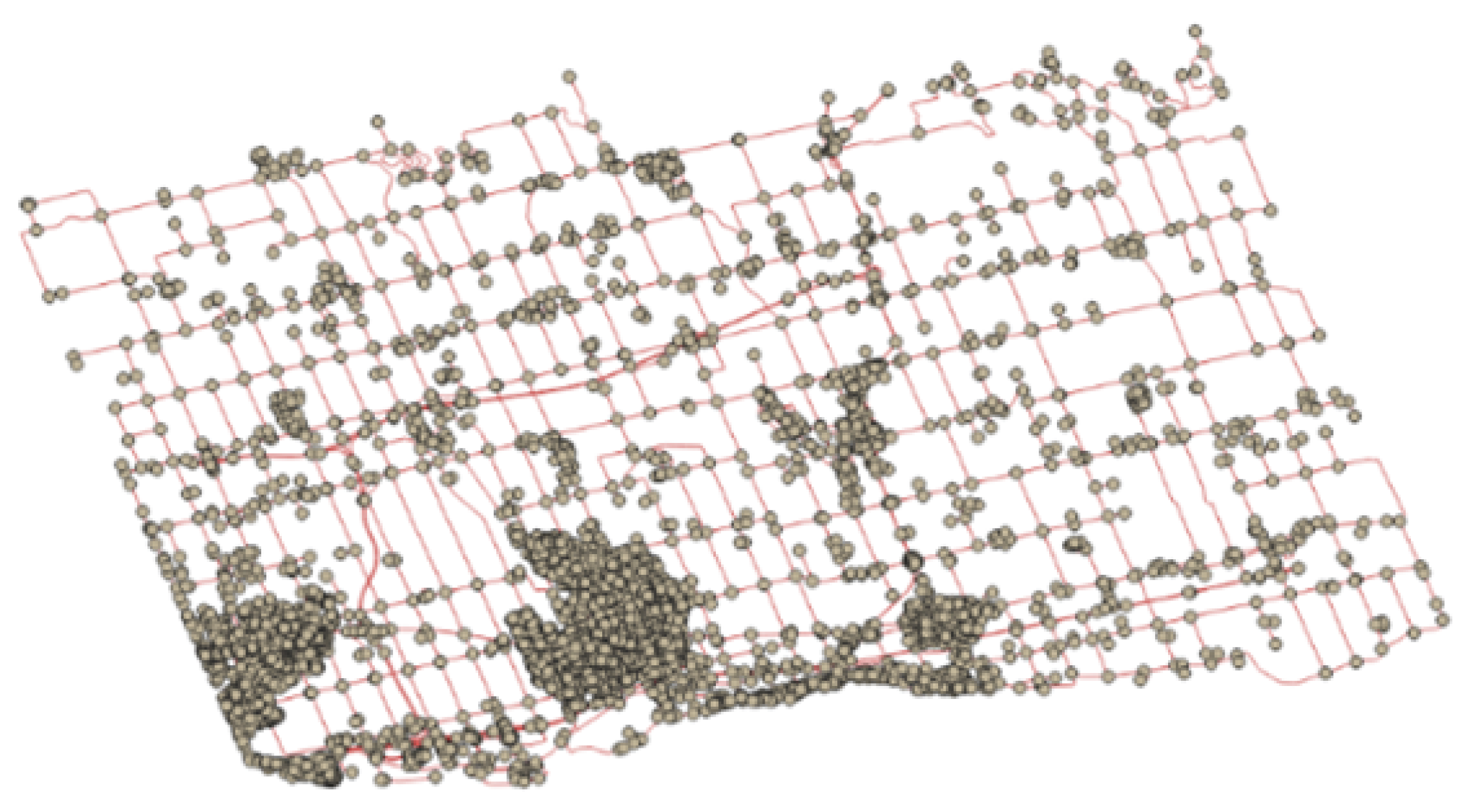
The entire map of the municipality was downloaded from the OSM database and analyzed in the QGIS environment. Figure 2 shows the QGIS graphical representation of this map, where the dots represent the intersections (nodes), and the lines represent the roads (edges).
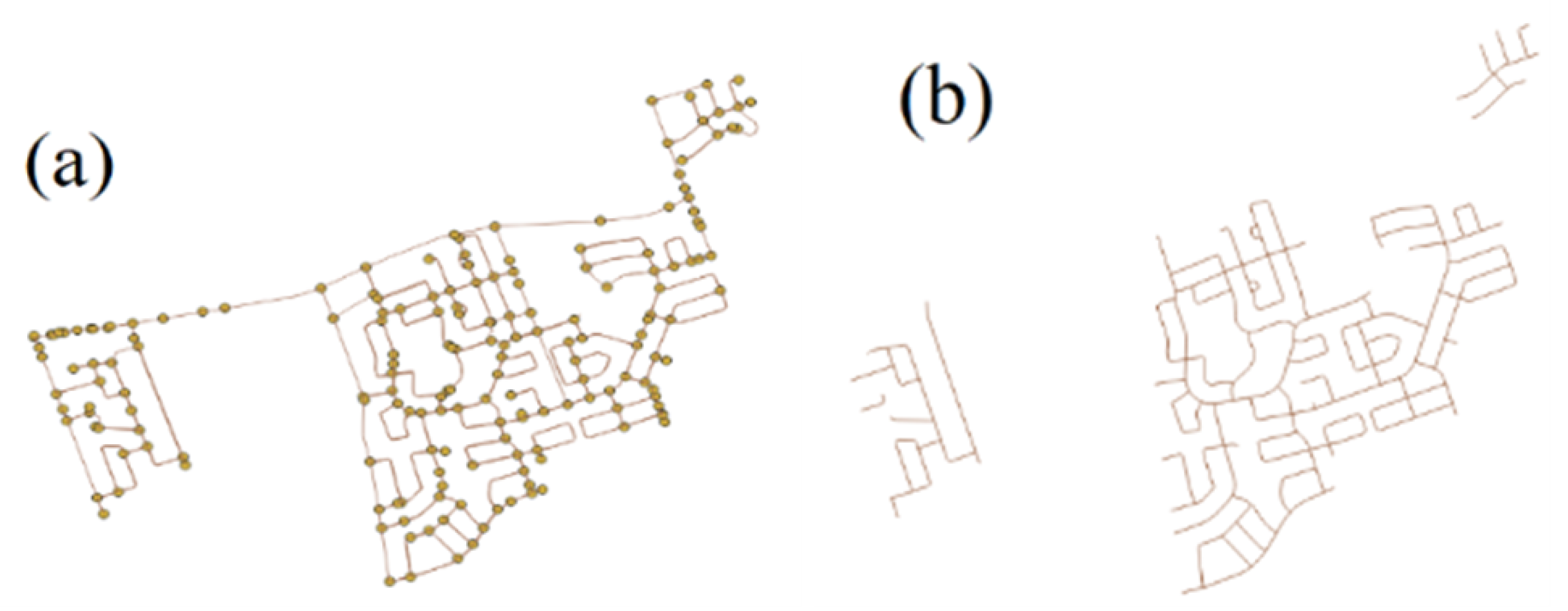
The entire map was divided into several sub-areas designated for each truck. This was performed by filtering out individual truck routes based on a comparison of the entire map with the city road network database. Figure 3 illustrates the OSM route for one of the operational trucks and one corresponding to Clarington’s network base. In this case, the whole municipality area was divided into 33 sub-areas for each of the 33 trucks, and a total of 3 depots were located within this area. The single-truck optimization approach was applied for each designated sub-area that was predefined by the city. In addition, the designated areas cover both single and multiple lane routes.
However, the first challenge was to solve the issue of network disconnectivity. Specifically, the road network in the city’s database is not connected at some points as shown in Figure 3b. This causes problems when generating the shortest paths. Therefore, the OSM was chosen to generate routes because it contains a fully connected map as illustrated in Figure 3a. However, the important attributes from the city road network such as roadway class, number of ways (one- or two-way street), etc., were transferred to the OSM routes. Note that extra edges in the OSM map are considered for traveling purposes only (non-serviced arcs). With a complete set of initial data (OSM routes) for each truck, which is a prerequisite to solving the optimal routing problem, shapefiles were generated to apply the optimization algorithm for 33 trucks. However, this paper presents the case of a single truck to elaborate on all the steps in the proposed method. A dataset of 10,359 edges and 6945 nodes was used in the study.

3. Methodology

This section explains a problem definition and the mathematical formulation of our selected algorithms. First, the problem for snowplow route optimization is described using graph theory, followed by the implementation of algorithms to solve it.

3.1. Problem Description and Objective Function

Snowplow route optimization is essentially a classical route inspection problem that can be explained using the graph theory as follows.
Let G ( V , E ) be a strongly connected multi-graph, where V is a set of nodes, and E is a set of directed edges. V = { v 0 , v 1 , v n } and E = ( v i , v j ) : v i , v j ϵ V , i < j , where v i and v j are the starting and ending node IDs of an edge, respectively, and i and j are the iterators for nodes. Their values depend on the number of nodes (length of network) present in the network for the considered service area. These values are greater than 0 and go up to the maximum number of nodes in the network presented. The limits of i and j are defined as v 0 i < v n 1 and j = i + 1 .
The first term in a node set, v 0 , is referred as the depot location. In this way, each node set carries a depot location as their first node. In graph theory, a multi-graph is a graph that carries parallel edges (multiple edges). Edges and nodes represent road segments and intersections, respectively, in this article. Each edge e = ( v i , v j ) ϵ E is associated with the non-negative travel distance c i j . The total travel distance of a route is the summation of each edge’s travel distance, c i j . The travel time for each road segment is represented as t i j . T i j = t i j , describing the accumulated time of the road network (route) that sums up each road segment travel time t i j .
The priority of road class for each road segment was also included in the problem. Roads in Class 1 have a higher priority than the rest. Often, the priority class of a road is determined by its traffic volume [8]. As a result, highways have a higher class than residential roads due to their higher traffic volume. However, the class of each road segment used in this study was predefined by the city.
To take into account the MMS, we defined an objective function that yields a higher value for servicing higher-class roads first rather than servicing in reverse order. The calculation of objective function values (i.e., fitness values) for these two opposite cases is illustrated in Figure 4, where the number between two nodes represents the travel distance (travel time) between them.
Aside from meeting the MMS requirement, our optimization function can also penalize the unsafe turns such as left-, U-, and sharp right turns that need to be avoided for safety and operational efficiency. The finalized objective function is divided into three parts. Equation (1) reflects the criteria of maximizing the MMS, whereas Equations (2) and (3) minimize the penalty of unsafe turns and total traveling distance, respectively.
M a x ( X i j · T i j )
M i n ( a · L t + b · U t + c · S t )
M i n ( d · c i j )
where a, b, c, and d are coefficients, and their values are determined by calculating the average of different types of turns for all the routes. The average of these turns provides a range of the fitness value and hence, the parameters are set to provide a reasonable penalty to stay within the range of the fitness value. L t , U t , and S t are the left, U-turn, and sharp right turns, respectively. The term X i j · T i j refers to the ‘value’ illustrated in Figure 4. T i j is the travel time across a road segment. X i j is the class of a road segment. X i j ϵ P is denoted by the range of P = 1 , , p , where p is the road class with the lowest priority, and the roads in Class 1 have a higher priority than the rest. The term a · L t + b · U t + c · S t represents the turning direction constraint, and c i j is the total distance in kilometers.
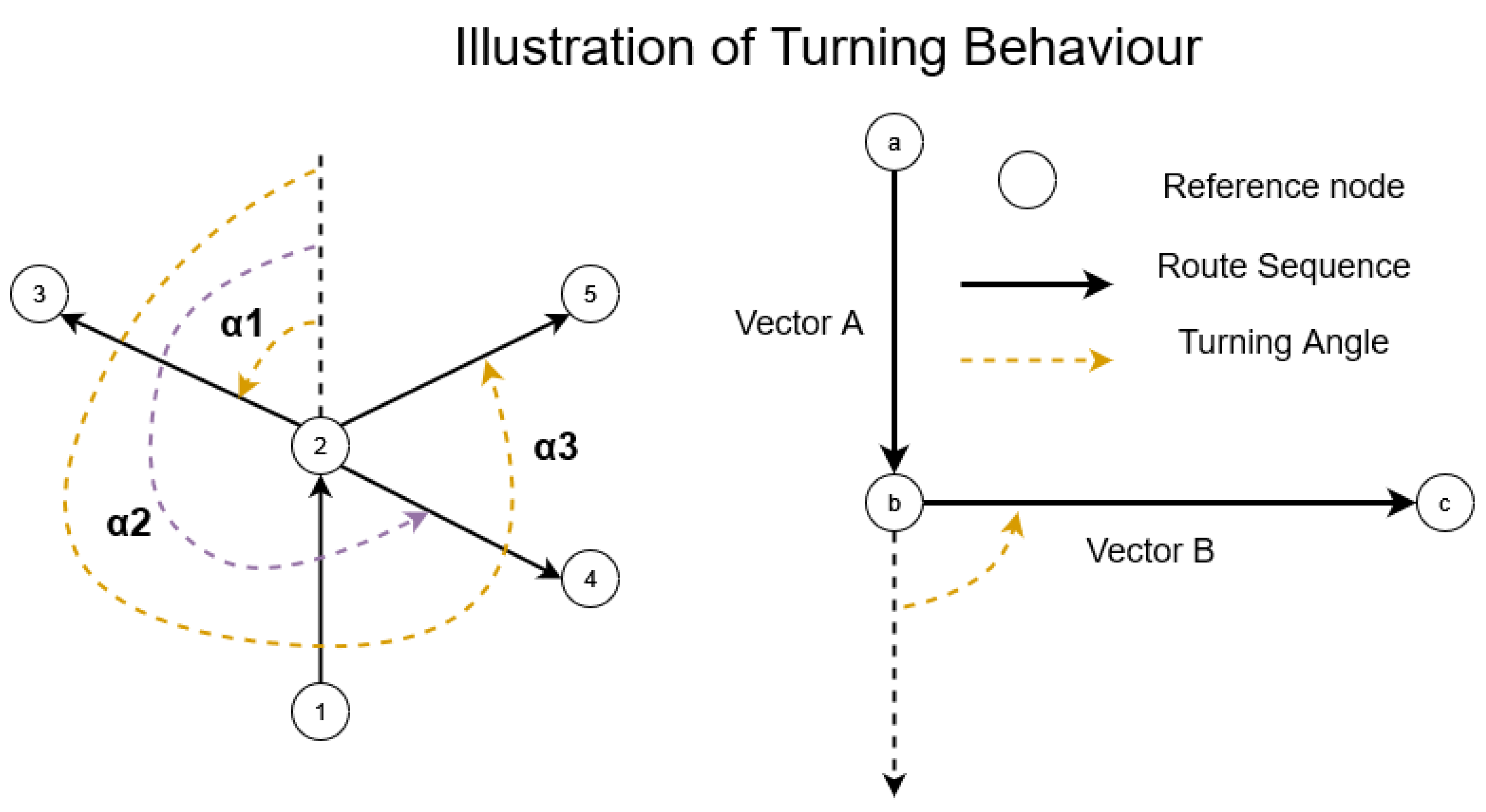
As another variable considered for the snowplow route optimization, the heading angle of a snowplowing truck can be calculated using the geographical information of longitude and latitude associated with each node and the cosine laws. When a truck reaches an intersection (node), its turning direction can be determined by calculating the angle between this node (i.e., current position of the truck) and the next node to which the truck is going.
Turning Type = left , i f 45 α 155 U , i f 155 < α 205 sharp right , i f 205 < α 240 right , i f 240 < α 315 straight , i f 315 < α 360 o r 0 α < 45
From Figure 5, V e c t o r A represents the vector from Node a to Node b, and V e c t o r B represents the vector from Node b to Node c. Then, cosine laws are used to calculate the resulting angle between the two vectors (i.e., α in a counterclockwise direction) which is defined as the turning angle. For each turn, α is calculated to identify the turning type. In Figure 5, α 1 , α 2 , and α 3 are the examples shown for left turn, right turn, and straight heading, respectively.
As the next step, the heading angles are categorized into different types of turns, i.e., left-, U-, sharp right-, right-, and straight turns defined based on the angle ranges in Equation (4). A combined result of Equations (1)–(3) determines the fitness value of this study.

3.2. Chinese Postman Problem

After translating the snowplow problem into the language of graph theory and defining the objective function and constraints, the next step is to tackle the Chinese Postman Problem, one of the well-known problems in graph theory.
A truck for snowplowing needs to travel along every edge in a graph while taking the shortest route possible. If a graph is Eulerian, all the nodes are of even degree; if a graph is Eulerian and each edge is traversed exactly once, it becomes a closed Eulerian circuit. A closed Eulerian circuit is the shortest circuit. However, snowplow routing problems are often complex in that some of the edges could be traversed more than once.
Given a connected undirected weighted graph G, the CPP computes a minimum cost-closed path that contains all edges at least once. However, in most cases, the graphs are not Eulerian, so CPP is useful for converting a non-Eulerian to an Eulerian graph. The CPP checks every node in a graph and adds an extra edge (i.e., act of traversing an edge without service) to the odd degree nodes to make them even. The steps of the CPP used in this study are presented in Algorithm 1. Let I be the set of vertices v i for which the number of incoming arcs exceeds that of outgoing arcs by s i and J, the set of vertices v j for which outgoing arcs outnumber incoming arcs by d j . Moreover, let a I J be the length of the shortest distance path from v i to v j . The CPP problem can be mathematically formulated as follows:
M i n i m i z e ( I J a I J · z I J )
where v i ϵ I and v j ϵ J .
Subject to
v J ϵ J z I J = s i
v i ϵ I z I J = d j
z I J 0
where the optimal z I J values represent the number of extra times each arc has to be traversed.
Algorithm 1 Chinese Postman Problem—Steps
     Input:  A n u n d i r e c c t e d c o n n e c t e d g r a p h G = ( V , E )
     Output:  A ( C P P ) t o u r T = ( n 1 , e 1 , n 2 , e 2 , , n i + 1 = n )
  • S t e p 1 : D e t e r m i n e i f G i s E u l e r i a n
  • S t e p 2 : i f G i s E u l e r i a n , o b t a i n a n E u l e r t o u r T
  • S t e p 3 : i f G i s n o t E u l e r i a n , f i n d a m i n i m u m c o s t a u g m e n t a t i o n o f G u s i n g
  • D i j k s t r a s t o c o n s t r u c t a n E u l e r i a n m u l t i g r a p h G a n d l e t T b e a n E u l e r t o u r o f G   S t o p
The best approach for adding extra edges is to check every odd degree node and find the shortest path between these nodes. If exactly two of the vertices are odd, Dijkstra’s algorithm is used to identify the shortest path between these two nodes. Then, extra edges are added in the circuit to accommodate the shortest path from Dijkstra’s algorithm and make the odd degree nodes even. As a result, the vehicle will have to go around the edges of this path twice and all other edges once. However, if more than two vertices are odd, what is required is to find the shortest paths between the odd degree node pairs. In this way, the odd degree nodes become even, and the minimal extra edges are added to the route.
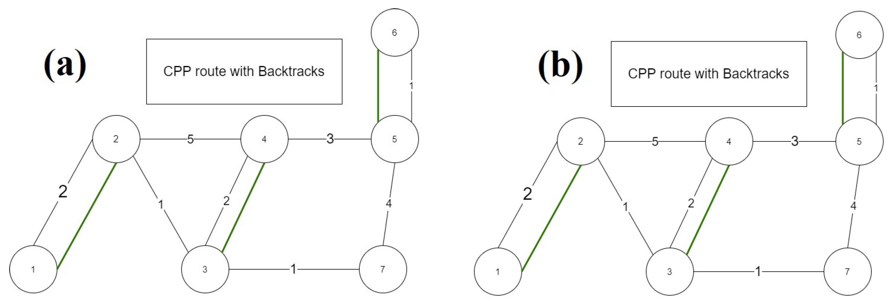
Figure 6 shows a simple example of converting a non-Eulerian graph to a Eulerian one. Figure 6a presents a non-Eulerian graph, while Figure 6b shows the minimum-weight expansion of the non-Eulerian graph to make it Eulerian. In the figure, every double (red) edge in the graph represents a backtrack. From the assumption that Node 1 is the starting and ending node for the closed tour, a possible solution obtained by applying the CPP algorithm is T = ( 1 , 2 , 4 , 5 , 6 , 5 , 7 , 3 , 4 , 3 , 2 , 1 ) with a total length of 24 by summing up the length of all traveled edges (i.e., the total distance traveled between nodes).

3.3. Dijkstra’s Algorithm

To find the shortest path between nodes (intersections), Dijkstra’s algorithm was implemented [20]. Dijkstra’s algorithm maintains a set of nodes whose final shortest-path weights from the source (depot location in our case) have already been determined. This algorithm repeatedly selects a node with the minimum shortest path estimate and relaxes all edges, leaving the selected node. Since Dijkstra’s algorithm solves a single-source shortest-path problem on a weighted and directed graph, it corresponds exactly to the snowplowing routing problem described in this study. The pseudocode of Dijkstra’s algorithm is presented below (Algorithm 2).
Algorithm 2 Dijkstra’s Algorithm
     Input:  g r a p h , s t a r t N o d e , t a r g e t N o d e
     Output:  p a t h
  • for n o d e i n g r a p h do
  •      n o d e . s c o r e : = i n f ;
  •      n o d e . s c o r e : = f a l s e ;
  • end for
  • s t a r t N o d e . s c o r e : = 0 ;
  • while T r u e do
  •      c u r r e n t N o d e : = n o d e W i t h L o w e s t S c o r e ( g r a p h )
  •      c u r r e n t N o d e . v i s i t e d = t r u e ;
  •     for  n e x t N o d e i n c u r r e n t N o d e . n e i g h b o r s  do
  •         if  n e x t N o d e . v i s i t e d = = f a l s e  then
  •             n e w S c o r e : = c a l c u l a t e S c o r e ( c u r r e n t N o d e , n e x t N o d e ) ;
  •            if  n e w S c o r e < n e x t N o d e . s c o r e  then
  •                 n e x t N o d e . s c o r e : = n e w S c o r e ;
  •                 n e x t N o d e . r o u t e T o N o d e : = c u r r e n t N o d e ;
  •            end if
  •         end if
  •     end for
  •     if  c u r r e n t N o d e = = t a r g e t N o d e  then
  •          r e t u r n b u i l d P a t h ( t a r g e t N o d e ) ;
  •     end if
  •     if  n o d e W i t h L o w e s t S c o r e ( g r a p h ) . s c o r e = = i n f  then
  •          t h r o w N o P a t h F o u n d ; ;
  •     end if
  • end while

3.4. Tabu Search Algorithm

After applying the CPP algorithm, the modified Tabu search algorithm [21] was used to optimize the routes using the objective function and constraints.
This algorithm is a metaheuristic optimization technique for optimizing model parameters. Like other metaheuristics techniques, it starts with an initial solution and proceeds iteratively by searching for immediate neighborhoods. Tabu search differs from local search in that it uses a memory to guide the search process.
One aspect of the memory use concerns a move between two adjacent solutions (also known as neighborhood). In order to avoid cycling or sticking in the local solution, space moves are declared Tabu for a specified number of iterations. In recent years, Tabu search has been applied successfully to many combinatorial optimization problems, especially in routing [21,22]. Algorithm 3 illustrates the pseudocode of the modified Tabu search algorithm applied in our study [21].
The Tabu search algorithm has three main memory structures that include the short-term memory, long-term memory, and the Tabu list [23]. Each factor fulfills its own defined task to reach the optimal solution.
Among them, the short-term memory performs the intensification, which prevents the algorithm from regenerating a previously generated solution. The long-term memory diversifies a solution by performing the exploration process. In addition, it generates a new solution to prevent being stuck in the sub-optimal dead end. The Tabu list keeps a record of previously visited solutions and facilitates the short-term memory to match the current solution with the previous one.
As seen in Algorithm 3, we consider a c u r r e n t s o l u t i o n (which is initialized with an input from the CPP algorithm) and compute a set of neighborhood solutions N ( c u r r e n t S o l u t i o n ) in each iteration. A neighborhood solution can be obtained through the permutation process with the current solution by swapping node positions (neighborhood).
Algorithm 3 Tabu Search algorithm
     Input:  A n i n i t i a l s o l u t i o n o f t r u c k r o u t e s , m a x i m u m i t e r a t i o n n u m b e r , l e n g t h o f t a b u
     Output:  T h e p o s s i b l e i m p r o v e d t r u c k r o u t e s
  • S t e p 1 : I n i t i a l i z a t i o n
  • S e t
  •      Current solution = Initial solution
  •      Current value = Initial value
  •      Best solution = Initial solution
  •      Best value = a large number
  •      Maximum number of iteration = a large number
  • S t e p 2 : F o r w a r d u p d a t i n g o b j e c t i v e f u n c t i o n v a l u e
  • for i t e r a t i o n n u m b e r = 1 : m a x i m u m i t e r a t i o n n u m b e r do
  •     while  B e s t v a l u e C u r r e n t v a l u e  do
  •          R a n d o m l y g e n e r a t e d i f f e r e n t n e i g h b o r h o o d s o l u t i o n s b a s e d o n
  •          t h e c u r r e n t s o l u t i o n u s i n g p e r m u t a t i o n
  •         Permutation Process
  •          C u r r e n t s o l u t i o n = B e s t f o u n d s o l u t i o n n o t i n t a b u
  •          C u r r e n t v a l u e = o b j e c t i v e f u n c t i o n ( c u r r e n t s o l u t i o n )
  •         if  B e s t v a l u e C u r r e n t v a l u e a n d C u r r e n t s o l u t i o n n o t i n t a b u l i s t  then
  •              B e s t s o l u t i o n = C u r r e n t s o l u t i o n
  •              B e s t v a l u e = C u r r e n t v a l u e
  •              a d d c u r r e n t s o l u t i o n t o t a b u l i s t
  •         end if
  •     end while
  • end for
When going from one solution to a neighborhood solution (move), the aim is to maximize the improvement of the objective function value (move value). Hence, the neighborhood solutions will be considered in decreasing order of their move value, and the non-Tabu neighbor solution with the best move value is chosen as the next current solution [22]. A solution is called Tabu if it has already appeared in the Tabu list. Therefore, the Tabu rule will be ignored if the neighborhood solution is Tabu but better than the current best solution.
The fitness value of each solution is calculated, and the best solution amongst the newly generated solutions is selected for the next iteration of the permutation. During the process, only nodes that are connected to the same edge are changed. In this way, the whole circuit remains connected, and a jump from one node to another disconnected node can be avoided.
Once the best solution is selected among the newly generated neighborhoods, it is verified whether this solution is better than the initial one. If a better solution is found, the permutation process is repeated to find another set of different neighborhoods; otherwise, a different combination of routes is searched through the process of merging and separating 243 edges. In the simulation, the fitness converged after 100 iterations, so this iteration number was set as a stopping criterion.
In Algorithm 3, the length of Tabu refers to the number of solutions stored in the Tabu list in each iteration. After randomly generating 24 different neighborhood solutions, the top five solutions are stored in the Tabu list, and the best solution among the randomly generated solutions is used for the next iteration.

4. Results and Discussion

This section discusses the network topology created using initial routes and analyses results obtained from the CPP algorithm. Then, we discuss the best routes generated from the optimization process by applying the Tabu search and Dijkstra’s algorithms with MMS and turning direction constraints.

4.1. Network Topology Generation

Network topology creation is the process of translating the city network database into IDE (Integrated Development Environment) readable format. This step was achieved using the NetworkX library [24], OSM, and QGIS. A map of Clarington was extracted from the OSM in the QGIS environment. QGIS exports shapefiles that the Networkx library can read and convert into graphs with nodes and edges in Python [25]. The generated graphs were used to implement the developed algorithms.
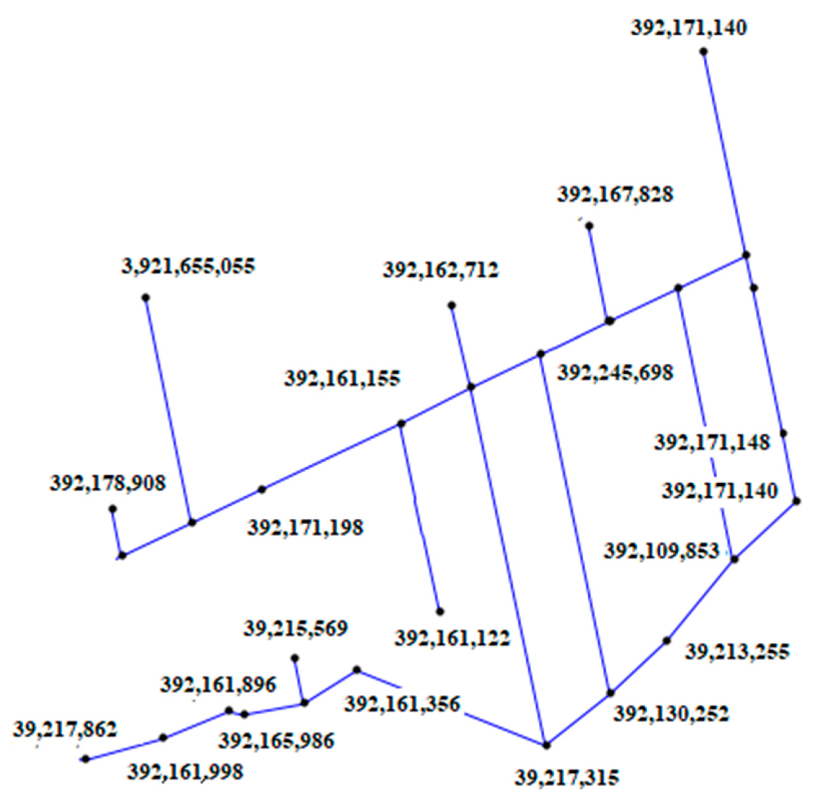
Figure 7 illustrates a network topology in Python graphing for one of the service trucks. The labeled numbers in the figure nodes indicate their IDs. Note that the attributes in the city road network database were transferred to the network topology during the creation of the graphs using the NetworkX library.

4.2. Results Obtained Using CPP and Dijkstra’s Algorithm

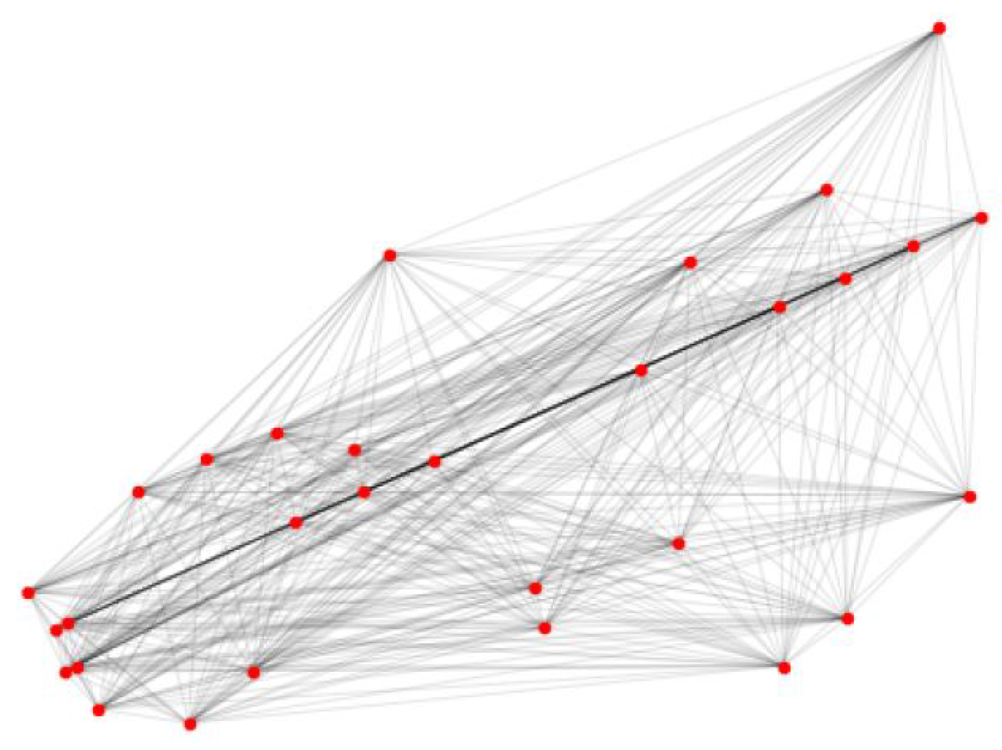
Following the creation of the network topology, Euler circuits for each truck’s route are constructed by applying the CPP algorithm. The CPP algorithm begins by identifying all odd degree nodes in a graph, and then it converts each odd degree node to an even degree node by adding parallel edges (backtracks) to create a Eulerian graph. The workflow of the CPP algorithm is described as follows. CPP first computes all possible pairs of odd degree nodes as shown in Figure 8. Red nodes in the network represent odd degree nodes. Edges with light gray represent possible pairs of odd degree nodes, while black edges are the actual edges of the network.
Second, the shortest path between odd degree nodes is calculated by applying Dijkstra’s algorithm [21,26] in order to minimize the backtracking distance and, therefore, reduce the overall circuit distance (find the shortest path). Note that the distance increases during the creation of a Eulerian circuit, but Dijkstra’s algorithm helps in minimizing it.
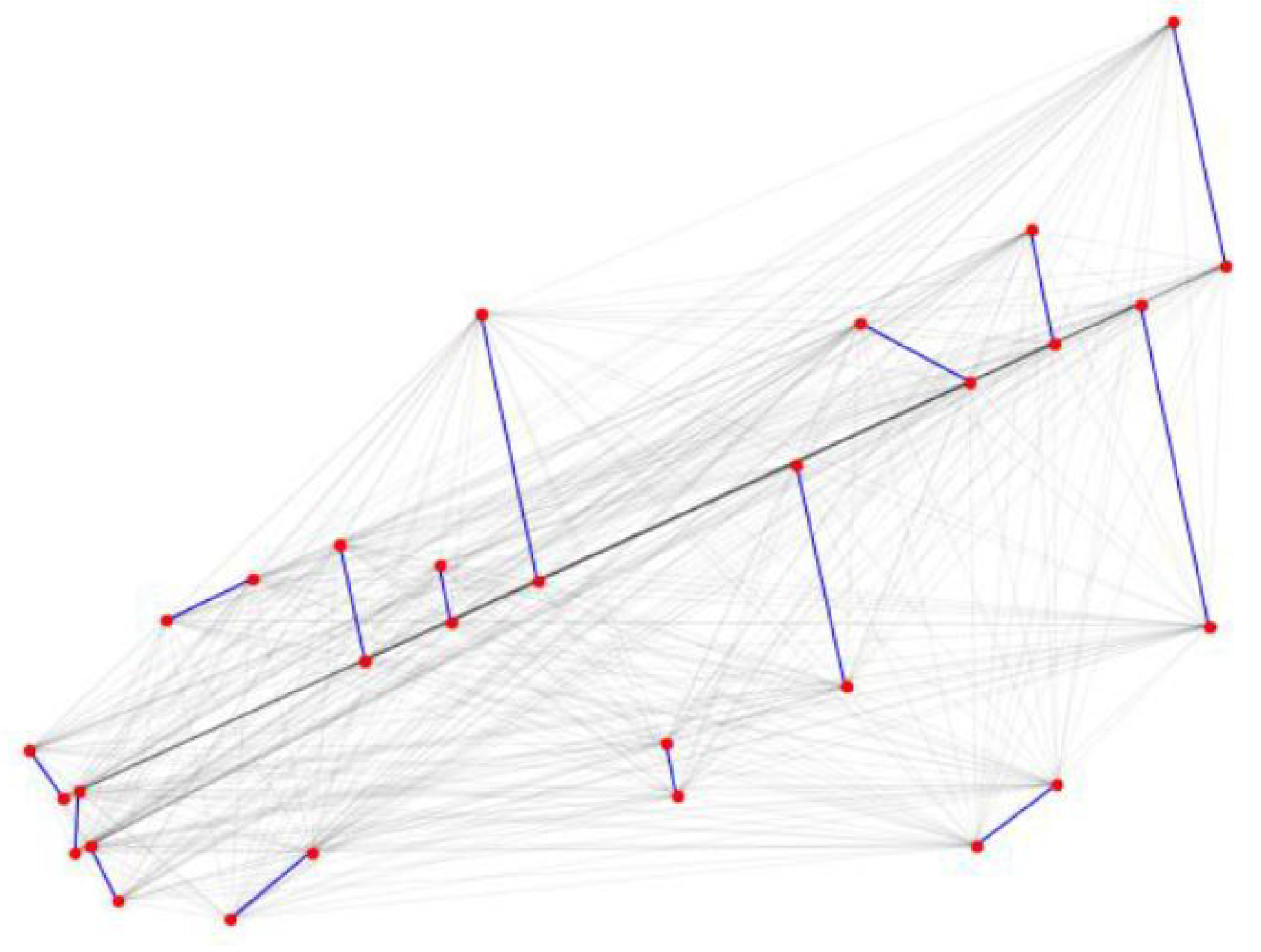
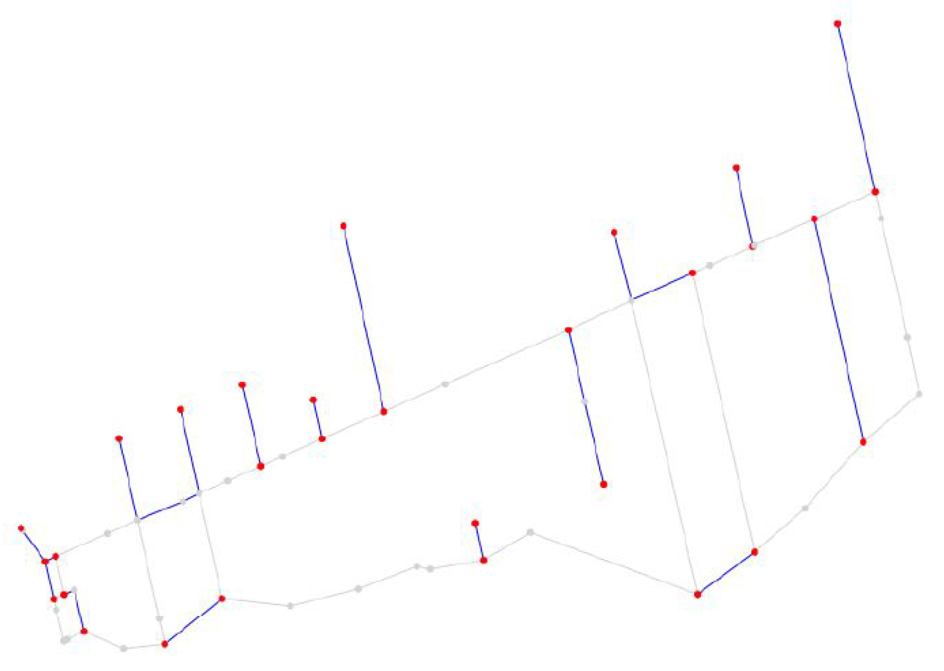
The final step in the CPP algorithm is to create a Eulerian circuit by adding backtracks obtained from the second step to the original circuit. Once we have the information about the possible shortest backtracks, the original network is updated by embedding the backtracked edges that are highlighted in blue in Figure 9.
By comparing Figure 8 and Figure 10, we can analyze that each blue (backtracked or in some cases, non-serviced edges) edge is connected to red (odd degree) nodes, which makes every odd degree node an even degree resulting in the overall Eulerian circuit.

4.3. Results of Optimization Algorithm

Optimal routes were obtained through the optimization process with the modified Tabu search algorithm and the assumed values, including the MMS listed in Table 1.
For the MMS, roadways should be serviced within the required (designated) time. The original time required by the MMS is shown in the table’s parentheses. However, since only one truck‘s service area was considered for the simulation, each time of the MMS was shortened to obtain reasonable results. For example, the original MMS time for road class is 4 h, but 1 h was assumed for simulation purposes.
Snowplowing trucks generally cover highways and municipal roads. The speed limit of municipal roads is 50 km/h in Clarington. However, the driving speed of trucks drops during snowplowing operations. Consequently, the assumed truck speed for simulations was 35 km/h.
As snowplow trucks are required to service roadways with single lanes and two-way roads, we considered both types of roads. If a road has two lanes (i.e., one for going and the other for coming back), it is presented with two edges covering both directions. For the generation of two lanes in the simulation, the same edge was duplicated, and then the nodes were swapped. For example, if an edge is starting from Node ‘a’ and ending at Node ‘b’, the second lane or the opposite direction lane starts from Node ‘b’ and ends at Node ‘a’. In this manner, all the attributes, such as distance, time, etc., remain the same, but the direction is reversed. The proposed method is also able to travel on non-serviced edges (deadhead travel).
To evaluate the optimization process, it is necessary to calculate the fitness value of the objective function in each iteration for every route. The route with the highest fitness value qualifies for the next iteration. After running the simulation several times, it was observed that the fitness value stayed nearly constant after 10 iterations; hence, for less computational cost, the stopping criteria was set to 10 iterations.
The routes obtained from the CPP method (Route 1) without optimization and the CPP with optimization (Route 2) are compared with respect to several criteria presented in Table 2.
Specifically, Route 1’s sequence was generated from the CPP and Dijkstra’s algorithm, while Route 2’s was with the combination of CPP, Dijkstra, and Tabu search algorithms. The Tabu search algorithm finds near-optimal solutions by swapping neighboring nodes (intersections) in every iteration of the permutation process. In this study, we swapped the nodes that are connected to at least three edges (roads).
The fitness value calculated from the objective function is affected by the MMS value and the number of left-, U-, and sharp right turns. By combining Equations (1)–(3), the objective function is designed such that a higher value of MMS and lower values of three unsafe turns and total distance would provide optimal solutions.
From Table 2, we can note that Route 2 offers a slightly better solution in terms of total travel time and distance than Route 1. Despite having one more left-turn, Route 2 has fewer U-turns and fewer roads that do not meet the MMS than Route 1.
Therefore, Route 2 provides a more economical and safer solution by reducing the travel distance/time and undesirable turns, as well as satisfying the MMS. The higher fitness value of Route 2 is indicative of satisfaction with the above comprehensive aspects (i.e., overall performance) that incorporate both traditional concerns (the shortest travel distance with the fewest backtracks) and actual operational constraints (eliminating unfavorable turning directions and meeting the MMS’s required service time).
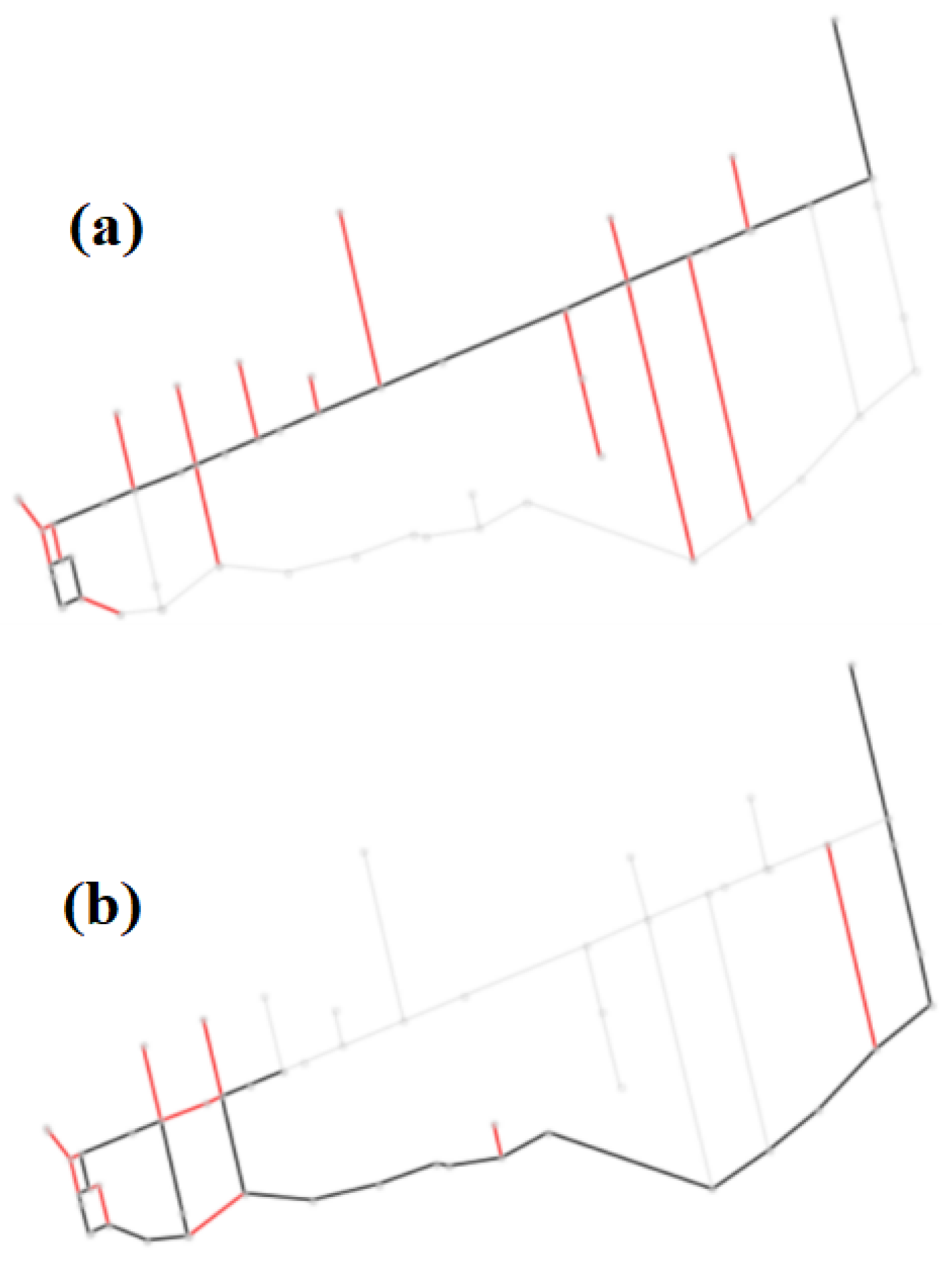
Figure 11 compares the route sequences of Route 1 and Route 2. In the figure, edges visited once are illustrated in black, while the ones visited twice (backtracks) are shown in red. Note that this figure is a screenshot of an animation showing the initial routing, and therefore some of the edges (light gray) are not yet traversed. As we can see, there is a sequence difference in that Route 1 attempts to cover the upper part first, while Route 2 begins with the lower part.
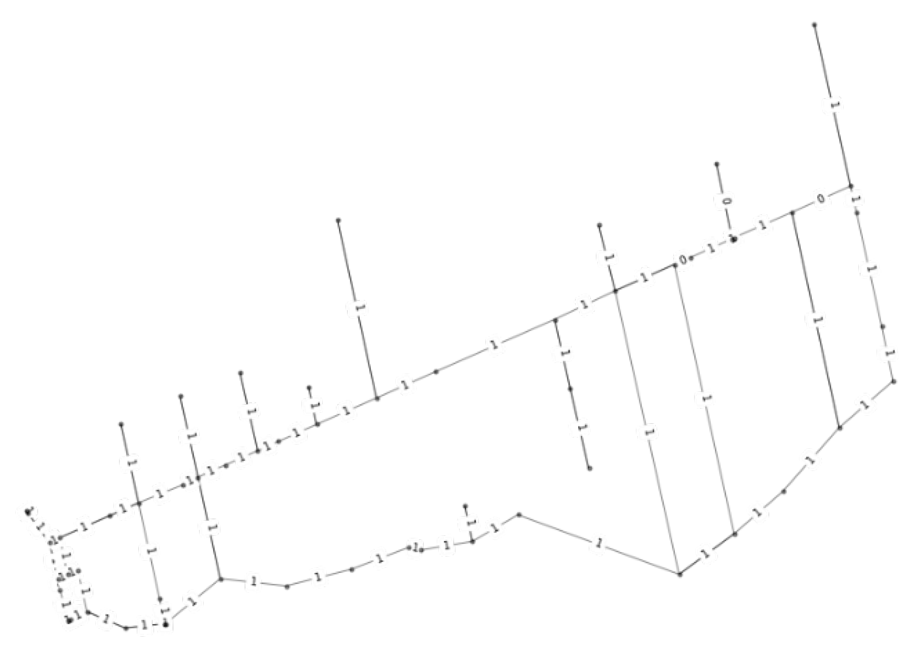
In Figure 12, roads (edges) served within the designated service time are labeled one, and those that do not meet this requirement have a label of zero.
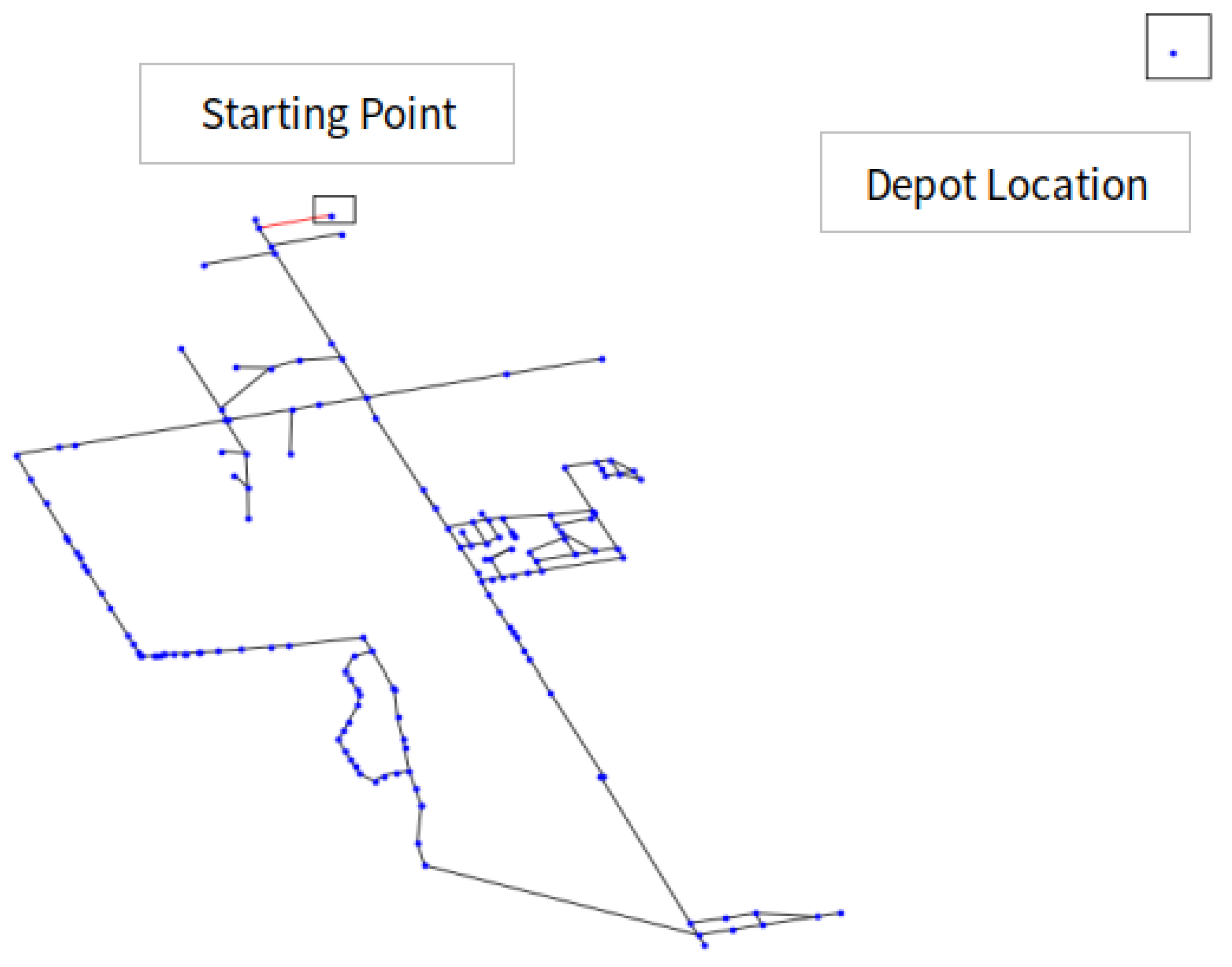
In the generated optimal route, a departure node for travel was chosen based on the shortest distance to the depot (i.e., the shortest distance to reach the designated service area).
Figure 13 indicates the locations of the departure node and depot that allow for the shortest distance between them in the considered service area.

5. Conclusions

The main objective of this study is to optimize residential snowplowing routes by considering the real-world operational constraints. For this, an initial network topology for each truck’s service area was generated using GIS data extracted from the OSM in the QGIS environment.
The city network’s attributes were then transferred to the initial network topology. The initial network topology containing the actual attributes was processed in Python by using the NetworkX library that converts the generated shapefiles to the IDE compatible graphing format. Then, the CPP algorithm was first applied to the initial routes for the generation of complete Eulerian circuits for each truck. This was achieved by adding backtracks to every odd degree node. In parallel with the CPP, Dijkstra’s algorithm was adopted to minimize the distance of backtracks by finding the shortest distance between the odd degree node pairs.
The Tabu search algorithm was also implemented to generate optimal routes by changing the immediate neighborhoods. In each iteration of the Tabu search algorithm, the fitness value of every route was calculated. Then, the route with the highest fitness value was chosen to generate further routes in the next iteration.
The objective function defined for the optimization took into account both MMS and turning direction. Namely, by increasing the fitness value, the road class priority for service can be met and the unsafe turning directions can be penalized.
Therefore, the generated optimal solutions represent the routes that ensure the shortest travel distance with the minimum deadheads and satisfy the required operational constraints including the MMS and unpreferred turns.
Due to our study being a simulation-based work, it is necessary to validate the proposed algorithm through field tests as a future extension that consider real-time traffic conditions and on-site weather conditions.
Future work will create new optimal routes by reassigning the existing routes to trucks, considering the workload balance between truck drivers as well as the operational constraints in the optimization process. In addition, the generated routes of the developed algorithms can be compared to those by other improved classical path planning algorithms, which can assist in understanding the advantages and disadvantages of the proposed methods.

Author Contributions

Writing—original draft preparation, A.R.; writing—review and editing, J.S.; technical advising, S.X. and T.J.K.; project administration, J.M.; data validation, C.B. All authors have read and agreed to the published version of the manuscript.

Funding

This research was funded by The Municipality of Clarington.

Institutional Review Board Statement

Not applicable.

Informed Consent Statement

Not applicable.

Data Availability Statement

Not applicable.

Acknowledgments

Not applicable.

Conflicts of Interest

The authors declared no potential conflict of interest with respect to the research, authorship, and/or publication of this article.

References

  1. Manual, H.C. Highway Capacity Manual. Washington, DC, USA. 2000. Available online: https://onlinepubs.trb.org/Onlinepubs/trnews/rpo/rpo.trn129.pdf (accessed on 28 July 2022).
  2. Jean, A.; Brian, M.; Jessica, A. Weather Information and Road Safety; Institute for Catastrophic Loss Reduction: Toronto, ON, Canada, 2001. [Google Scholar]
  3. Rao, T.; Mitra, S.; Zollweg, J.; Sahin, F. Computing optimal snowplow route plans using genetic algorithms. In Proceedings of the IEEE Systems, Man, and Cybernetics (SMC), Anchorage, AK, USA, 9–12 October 2011; pp. 2785–2790. [Google Scholar]
  4. Applegate, D.; Bixby, R.; Chvatal, V.; Cook, W. The Traveling Salesman Problem; Princeton University Press: Princeton, NJ, USA, 2011. [Google Scholar]
  5. Rao, T.; Mitra, S.; Zollweg, J. Snow-plow route planning using AI search. In Proceedings of the IEEE Systems, Man, and Cybernetics (SMC), Anchorage, AK, USA, 9–12 October 2011; pp. 2791–2796. [Google Scholar]
  6. Malandraki, C.; Daskin, M. The maximum benefit Chinese postman problem and the maximum benefit traveling salesman problem. Eur. J. Oper. Res. 1993, 65, 218–234. [Google Scholar] [CrossRef]
  7. Perrier, N.; Langevin, A.; Amaya, C. Vehicle routing for urban snow plowing operations. Transp. Sci. 2008, 42, 44–56. [Google Scholar] [CrossRef] [Green Version]
  8. Kinable, J.; van Hoeve, W.; Smith, S. Optimization models for a real-world snowplow routing problem. In Proceedings of the International Conference on AI and OR Techniques in Constraint Programming for Combinatorial Optimization Problems, Banff, AB, Canada, 29 May–1 June 2016; pp. 229–245. [Google Scholar]
  9. Sullivan, J.; Dowds, J.; Novak, D.; Scott, D.; Ragsdale, C. Development and application of an iterative heuristic for roadway snow and ice control. Transp. Res. Part A Policy Pract. 2019, 127, 18–31. [Google Scholar] [CrossRef]
  10. Çodur, M.; Yılmaz, M. A time-dependent hierarchical Chinese postman problem. Cent. Eur. J. Oper. Res. 2020, 28, 337–366. [Google Scholar] [CrossRef]
  11. Korteweg, P.; Volgenant, T. On the hierarchical Chinese postman problem with linear ordered classes. Eur. J. Oper. Res. 2006, 169, 41–52. [Google Scholar] [CrossRef]
  12. Ahabchane, C.; Langevin, A.; Trépanier, M. Robust optimization for the hierarchical mixed capacitated general routing problem applied to winter road maintenance. Comput. Ind. Eng. 2021, 158, 107396. [Google Scholar] [CrossRef]
  13. Bopardikar, S.D.; Englot, B.; Speranzon, A. Multiobjective path planning: Localization constraints and collision probability. IEEE Trans. Robot. 2015, 31, 562–577. [Google Scholar] [CrossRef]
  14. Ontario. Minimum Maintenance Standards for Municipal High-Ways. Available online: https://www.ontario.ca/laws/regulation/020239 (accessed on 23 January 2022).
  15. Minieka, E. The Chinese postman problem for mixed networks. Manag. Sci. 1979, 25, 643–648. [Google Scholar] [CrossRef]
  16. Dijkstra, E.W. A note on two problems in connection with graphs. Numer. Math. 1959, 1, 269–271. [Google Scholar] [CrossRef] [Green Version]
  17. Ahr, D.; Reinelt, G. A Tabu search algorithm for the Min–Max k-Chinese postman problem. Comput. Oper. Res. 2006, 33, 3403–3422. [Google Scholar] [CrossRef]
  18. OpenStreetMap. OpenStreetMap Data. Available online: https://www.openstreetmap.org (accessed on 23 January 2022).
  19. Qgis.org. QGIS. Available online: https://www.qgis.org/en/site (accessed on 23 January 2022).
  20. Sniedovich, M. Dijkstra’s algorithm revisited: The dynamic programming connexion. Control Cybern. 2006, 35, 599–620. [Google Scholar]
  21. Xu, S.; Kwon, T. Optimizing snowplow routes using all new perspectives: Road users and winter road maintenance operators. Can. J. Civ. Eng. 2020, 48, 1–10. [Google Scholar] [CrossRef]
  22. Ghiani, G.; Guerriero, F.; Laporte, G.; Musmanno, G. Tabu Search Heuristics for the Arc Routing Problem with Intermediate Facilities under Capacity and Length Restrictions. J. Math. Model. Algorithms 2004, 3, 209–223. [Google Scholar] [CrossRef]
  23. Glover, F. Tabu Search: A Tutorial. Interfaces 1990, 20, 74–94. [Google Scholar] [CrossRef]
  24. NetworkX. NetworkX Documentation. Available online: https://networkx.org (accessed on 23 January 2022).
  25. Rasul, A.; Seo, J.; Xu, S.; Kwon, T.; MacLean, J.; Brown, C. Snowplow route optimization using Chinese postman problem and Tabu search algorithm. In Proceedings of the ISARC 2021, Dubai, United Arab Emirates, 2–4 November 2021; pp. 403–409. [Google Scholar]
  26. Cormen, T.; Leiserson, C.; Rivest, R.; Stein, C. Introduction to Algorithms; The MIT Press: Cambridge, MA, USA, 2001; pp. 658–664. [Google Scholar]
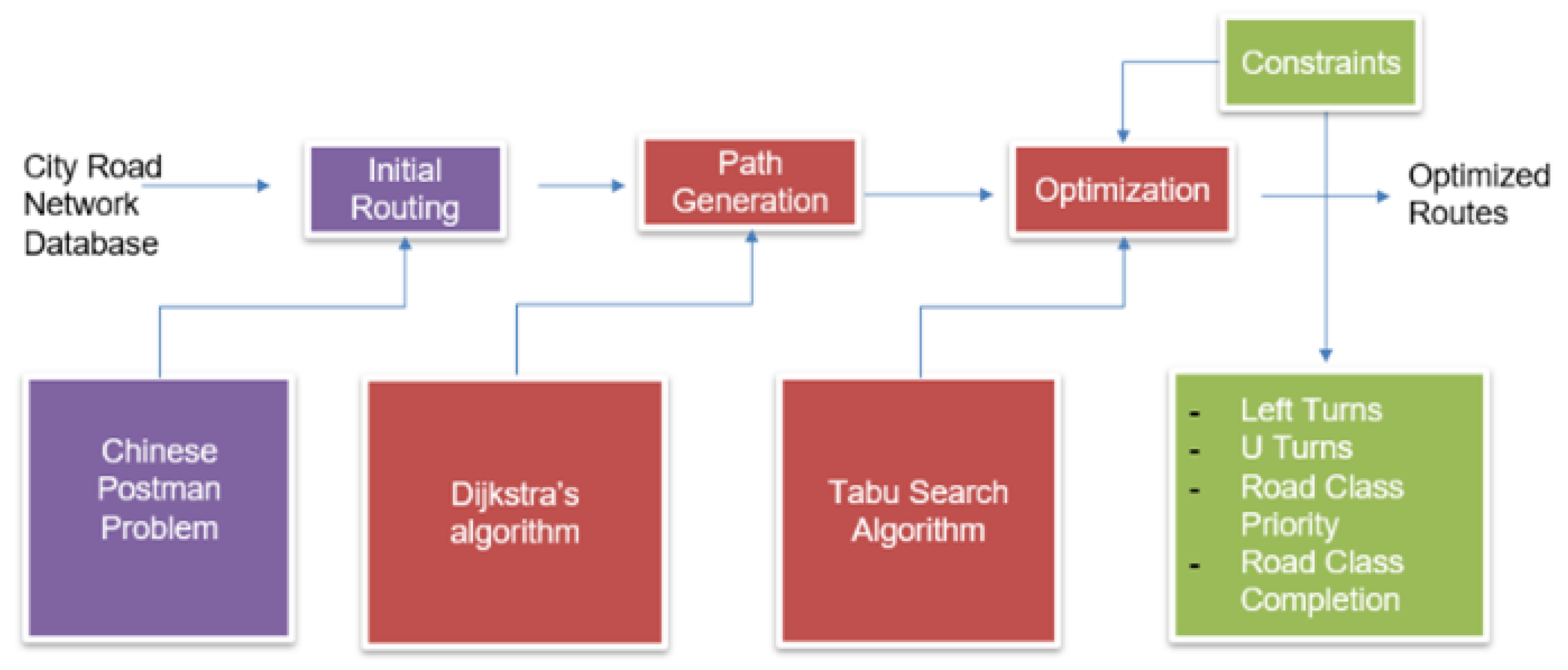
Figure 1. Framework for snowplow route optimization.
Sustainability 14 13130 g001
Figure 2. Graphical OSM map containing the roads and intersections of the targeted municipality.
Sustainability 14 13130 g002
Figure 3. Route comparison between OSM and the city’s network database: (a) route for an operational truck in OSM; and (b) corresponding route in Clarington’s network database for (a).
Sustainability 14 13130 g003
Figure 4. A comparison of routing sequences for the MMS: (a) calculation of an objective function value to first consider higher-class roads; and (b) calculation of an objective function value to first consider lower-class roads.
Sustainability 14 13130 g004
Figure 5. The defined turning directions according to angle ranges.
Sustainability 14 13130 g005
Figure 6. Conversion of a Non-Eulerian graph to an Eulerian one: (a) example of non-Eulerian graph; and (b) minimum-weight expansion of (a) to make it Eulerian.
Sustainability 14 13130 g006
Figure 7. Network topology in Python graphing.
Sustainability 14 13130 g007
Figure 8. Possible pairs of odd degree nodes.
Sustainability 14 13130 g008
Figure 9. The shortest path among pairs of odd degree nodes.
Sustainability 14 13130 g009
Figure 10. Eulerian circuit—backtracks added to the original network.
Sustainability 14 13130 g010
Figure 11. Comparison of the routes sequence between CPP (Route 1) and CPP with optimization (Route 2): (a) Route 1: CPP and (b) Route 2: CPP + optimization.
Sustainability 14 13130 g011
Figure 12. Indication of the MMS satisfaction on the map: 1—Routes plowed within the designated class time. 0—Routes plowed after the designated class time.
Sustainability 14 13130 g012
Figure 13. Locations of the departure node and depot in the considered service area consideration.
Sustainability 14 13130 g013
Table 1. The variables used for the optimization and their assumed values.
VariableAssumed Value
Truck speed35 km/h
Service areaClarington
Number of trucks1
MMS:
applicable time for
road class 1
1 h for simulation
(original time: 4 h)
MMS:
Applicable time for
road class 2
2 h for simulation
(original time: 6 h)
MMS:
Applicable time for
road class 3
3 h for simulation
(original time: 12 h)
MMS:
Applicable time for
road class 4
4 h for simulation
(original time: 16 h)
MMS:
Applicable time for
road class 5
5 h for simulation
(original time: 24 h)
Number of lanesBoth single and multi-lanes covered
Table 2. Comparison between routes obtained from simulations.
RoutesRoute 1: CPPRoute 2: CPP + Optimization
Fitness−2060
Total travel Time1 h 17 min1 h 15 min
Total travel distance (km)63.462.9
Left Turns2122
U-turns129
Sharp Right Turns00
Number of roads (edges) failing to the MMS43
Publisher’s Note: MDPI stays neutral with regard to jurisdictional claims in published maps and institutional affiliations.