An Integrated Sensitivity and Uncertainty Quantification of Fragility Functions in RC Frames

Abstract

Uncertainty quantification is a challenging task in the risk-based assessment of buildings. This paper aims to compare reliability-based approaches to simulating epistemic and aleatory randomness in reinforced concrete (RC) frames. Ground motion record-to-record variability is combined with modeling uncertainty which is propagated by either an approximate first-order second-moment or Latin Hypercube sampling methods. The sources of uncertainties include post-yield hardening stiffness, cyclic energy dissipation capacity, and the plastic and post-cap rotation capacities of beam-column elements. All nonlinear simulations are performed with two methods: detailed incremental dynamic analysis, and the simplified SPO2IDA. The combination of all parametric methods is used to analyze two RC frames (four-story and eight-story), and the results are further post-processed to drive fragility functions. Several assumptions were investigated in curve fitting, functional form, uncertainty, and confidence intervals. The results indicate the importance of modeling uncertainty in higher seismic intensity levels. While there is a negligible difference in fragility curve fitting, its variability due to optimal intensity measure parameters is dominant.

1. Introduction

Because the concurrent investigation of aleatory and epistemic uncertainties is computationally expensive, many researchers have proposed a separate uncertainty quantification (UQ) framework for each source and combined them afterward [1,2,3]. Such a simplification essentially ignores the interaction of various sources of uncertainties. The concept of UQ is well integrated within the performance-based earthquake engineering (PBEE) framework proposed by Pacific Earthquake Engineering Research Center (PEER) [4]. This framework connects the four chains of seismic hazard analysis, structural analysis, damage analysis, and loss analysis to provide engineers and stakeholders with the required decision-making tools.

1.1. Literature Review

The introduction of the incremental dynamic analysis (IDA) method by Vamvatsikos and Cornell [5] facilitated the seismic performance evaluation of structures. The uncertainties associated with ground motions in the IDA method have been investigated by Jalayer [6]. The epistemic-type uncertainties can be divided into several groups. The most important ones are material and modeling uncertainties [7]. In the case of modeling uncertainties. Research began in the 1980s with the pioneering work of Ellingwood [8] on calculating the statistics of the modeling parameters such as strength capacity, displacement capacity, and stiffness. Ibarra et al. [9] introduced the modeling parameters in the moment–curvature diagram using the results of experimental tests. Panagiotakos and Fardis [10] and Haselton et al. [11] provided several analytical equations to estimate different modeling parameters.

Lignos et al. [12] investigated the seismic performance of a four-story steel frame and predicted the probability of collapse due to earthquake load. They considered the plastic rotation, ${\theta }_p$, and post-cap rotation, ${\theta }_{pc}$ of the moment–curvature diagram in beams and columns among the modeled random variables with log-normal distributions. To facilitate their simulations, they adopted a random perturbation method to combine the ground motion record-to-record (RTR) variability with modeling uncertainty. In this method, 400 sets of data for ${\theta }_p$ and ${\theta }_{pc}$ were generated using the Monte Carlo simulation (MCS) method, and a random ground motion record was selected from the defined “record pool” and assigned to each model. Using the first order-second moment (FOSM) method, mean values were assigned to each of the random variables (RVs) separately to perform the sensitivity analysis. In this method, the dispersion of collapse capacity was derived from the square root of the sum of squares of the resulting dispersion of aleatory and epistemic uncertainties. Moreover, the sensitivity to three values of correlation coefficients was assessed in [12]. The production of datasets was performed separately for three correlation coefficients of 0.3, 0.6, and 1.0, and was compared with the benchmark case which merely considered the RTR uncertainty. The results showed that modeling uncertainties significantly increase the likelihood of collapse (from %3 initially to about 18%) with a higher effect due to ${\theta }_p$ as compared with ${\theta }_{pc}$.

Haselton and Deierlein [13] studied the seismic performance of reinforced concrete (RC) frames with various design philosophies. Several element modeling parameters, such as ${\theta }_p$, ${\theta }_{pc}$, the ratio of capping moment to yield moment ($M_c/M_y$), and cyclic deterioration capacity ($\lambda$) were assumed to be RV. In combination with the IDA method and FOSM approximation, they evaluated the effects of modeling uncertainties on the fragility curves. While the FOSM method did not affect the median, it caused a significant change in the tail of the fragility curve. In similar research, Khojastehfar et al. [14] estimated the collapse fragility curves of a three-story steel moment frame by combining the MCS and IDA methods. They concluded that the mean value of the resulting fragility curves diminished, while the standard deviation (STD) was observably augmented. Asgarian and Ordoubadi [15] studied the effects of the damping ratio, mass, yield strength, and ultimate strength as uncertainty sources on two five-story special and ordinary steel moment frames. They adopted Latin Hypercube sampling (LHS) for seismic reliability analysis and reported an apparent decrease in the seismic performance of the frames by considering epistemic uncertainties.

Ricci et al. [16] examined three RC frames designed according to the Italian building code and investigated the effect of story numbers, site hazard, infill masonry panel types, and lateral resisting systems on seismic performance through pushover analysis (POA) and dynamic simulations. Their study revealed that the site hazard had the most influence on the seismic performance of the studied frames. However, the effects of infill type and distributions in the structure were remarkable as well. Badalassi et al. [17] investigated the effects of the mechanical properties of elements, including various lateral moment-resisting systems and steel qualities in steel and steel–concrete composite structures, on the seismic performance of fifteen structures. Their study accented the dependable results of the Eurocode design method [18] at seismic performance safety levels. Barbato et al. [19] compared the results of the direct differentiation-based FOSM method with MCS and experimental data in two simply supported and non-symmetric two-span continuous composite beams. It was shown that a high level of material nonlinearity makes the results of FOSM and MCS incompatible. While the impact of the modeling uncertainties on seismic performance of the structures is evident, multiple studies [20,21,22,23] have shown that its effect is more pronounced at higher performance levels, especially at the collapse limit state (LS).

There are multiple considerations concerning the simultaneous evaluation of epistemic and aleatory uncertainties: (1) at a higher LS (or even a higher seismic intensity level), the impact of modeling uncertainties on the seismic response of the structural system is more significant compared to a lower LS; (2) the contribution of aleatory uncertainty in the seismic response of the structures is greater than epistemic uncertainties at all LSs [24]; (3) the key factors in evaluating the impact of modeling uncertainties on the structure’s seismic response are (3a) the underpinning assumptions and methodologies, (3b) the spatial correlation considerations, and (3c) adoption of proper experimental results to develop realistic numerical models [21].

While the first fragility curves were developed back in the 1980s by Kennedy et al. [25], the most notable is a work by Shinozuka et al. [26]. Following these pioneering works, thousands of researchers have developed fragility functions (not strictly for seismic hazards) for various types of engineering structures. Baker [27] investigated different analysis techniques, such as IDA, multiple stripe analysis (MSA), and lognormal cumulative distribution function (CDF) fittings. Lallemant et al. [28] expanded this study for generalized linear models with probit and logistic functions. Miano et al. [29] developed the concept of robust fragility functions using both IDA and Cloud methods. In addition to the lognormal CDF model, several researchers have proposed non-parametric methods to develop fragility functions [30].

Other researchers have focused on assessing the uncertainties associated with developing a fragility function based on different assumptions. Iervolino [31] discussed the impact of sample variability in fragility functions and the resulting seismic structural risk. Baraschino et al. [32] further studied the uncertainty in the fragility curve using different methods such as bootstrap and delta methods. The impacts of the number of initial records and nonlinear transient analyses were studied by Baltzopoulos et al. [33]. De Risi et al. [34] showed the variability in developed fragility curves with multiple limit state assumptions. Basone et al. [35] studied the role of both stationary and non-stationary artificial ground motions in the fragility assessment of RC frames using the IDA method.

1.2. Research Gap and Contributions

As discussed in the Literature Review, many factors are involved in developing a seismic fragility function. While researchers typically account for many of those factors, the developed fragility function might be different from the true yet unknown one. To the best of the authors’ knowledge, there is no unique research that has collected all the factors affecting the fragility of a structural system in one way or another. Moreover, there are limited studies that have evaluated the sensitivity of the fragility functions to the major assumptions made during their development. Finally, the potential interaction of different assumptions, simplifications, and analysis methods have not been addressed properly in previous research. This is a major research gap in seismic risk assessment of reinforced concrete structures, which eventually affects the credibility of the outcome. Subsequently, it affects disaster management plans for mitigating the devastating consequences of seismic hazards to the community.

Therefore, the objective of this paper is to develop the seismic fragility functions for two medium and high-rise RC frames by integrating different combinations of aleatory and epistemic uncertainty sources, uncertainty propagation methods, structural analysis techniques, fragility function fitting, etc. All the methods that are used in this paper are valid assumptions an analyst may use during a real-world risk assessment project. Therefore, it is important to have a good understanding of the uncertainty and bias terms that each method (or combination of them) may cause in the fragility functions.

More specifically, the following factors are considered in this paper: (1) frames with different heights; (2) two uncertainty sources, i.e., RTR variability and modeling randomness; (3) two analysis techniques, i.e., detailed IDA and simplified SPO2IDA; (4) two reliability analysis methods, i.e., efficient LHS and approximate FOSM (including their comparison to estimate the IM-variant IDA fractile values); (5) various limit states; (6) sensitivity of LHS-based IDA collapse capacity points; (7) five methods for fragility curve fitting; (8) robust fragility functions, confidence intervals, and fragility surfaces; (9) dependency of median and dispersion of fragility functions to the engineering demand parameter and choice of intensity measure parameter (from a pool of sixteen alternatives); and (10) model parameter correlation both within the element and between elements.

This paper begins with a general review of the underpinning theories in reliability analysis and fragility functions in Section 2, followed by a short description of their implementation in Section 3. The frames used as the case study are discussed in Section 4. Finally, our results and findings are presented in Section 5.

2. Underpinning Theory

2.1. Reliability-Based Analysis

As researchers in previous studies have elaborated on different methods of seismic reliability analysis [36,37], we only provide a brief review of two adapted methods: (1) the first order-second moment reliability method (FOSM) and (2) Latin Hypercube sampling (LHS) [38].

2.1.1. FOSM

The FOSM method is the simplest seismic reliability analysis procedure; it provides a linear approximation of the structural response concerning fluctuations in RVs. In this method, a “Base Case” is defined in which all RVs are set in their mean $\mu$ values, as follows:

$${\mu }_{lnRes}=g\left({\mu }_{lnR{V}_1},{\mu }_{lnR{V}_2},\dots ,{\mu }_{lnR{V}_N}\right)$$

(1)

Next, all the RVs are selected one by one. For each $R{V}_i$, only its value is changed by a scalar perturbation coefficient (in this paper, by one standard deviation (STD)), while others are kept in their mean values. The resulting “Uncertain Case” is re-analyzed. The response of the structure in the Uncertain Case is combined with Base Case response usingthe classic FOSM equation:

$${\sigma }_{lnRes}^2\approx \sum _{i=1}^N\sum _{j=1}^N{\left.\begin{array}{c}\frac{\partial g}{\partial lnR{V}_i}\end{array}\right|}_{{\mu }_{lnRV}}{\left.\begin{array}{c}\frac{\partial g}{\partial lnR{V}_j}\end{array}\right|}_{{\mu }_{lnRV}}{\rho }_{lnR{V}_{i}lnR{V}_j}{\sigma }_{lnR{V}_i}{\sigma }_{lnR{V}_j}$$

(2)

where ${\left.\begin{array}{c}\frac{\partial g}{\partial lnR{V}_i}\end{array}\right|}_{{\mu }_{lnRV}}$ is approximated linear in FOSM formulation, as follows:

$${\left.\begin{array}{c}\frac{\partial g}{\partial lnR{V}_i}\end{array}\right|}_{{\mu }_{lnRV}}\approx \frac{ln\left(Re{s}_2\right)-ln\left(Re{s}_1\right)}{{\sigma }_{lnR{V}_i}}$$

(3)

It must be noted that in this study, the FOSM approximation is calculated in a semi-logarithmic space, and the above formulation is based on this assumption. This is because the natural logarithm of the structural responses has a better correlation (i.e., linear approximation) with RVs compared to using simple Cartesian space [39,40,41].

2.1.2. LHS

The LHS method is one of the sample reduction simulation-based techniques widely used in structural reliability. In this method, the cumulative distribution function (CDF) of each RV is partitioned into N identical sections, which presents the number of samples. A representative from each section is chosen, and the corresponding value of RV is obtained from the probability distribution function (PDF). This effort finally results in a matrix containing the events of each RV, all of which have the same number of N samples. The last step is to perturb this matrix in such a way that the correlation matrix of the final dataset becomes nearly identical to the desired one defined by the user. Different techniques can be used for perturbation, such as a simulated annealing algorithm, translational propagation algorithm, or enhanced stochastic evolutionary algorithm.

In this paper, the LHS method is applied using the lhsdesign function in Matlab [42]. This function generates a matrix $[N,M]$, in which N is the number of samples and M presents the number of RVs. Because the matrix generated by lhsdesign is uniform and bounded to [0, 1], an appropriate method should be used to transfer this matrix into the desired space. This can be easily achieved using the following algorithm [43,44]:

• Convert the initially generated matrix to data in standard normal space using the probability preserving equation [5]:

  $$y_i={\mathrm{\Phi }}^{-1}\left(U\left(u_i\right)\right)$$

  (4)
• Convert the desired correlation matrix to a correlation matrix that is compatible with a space similar than the standard normal space, except that the correlation matrix is not the identity matrix per the NATAF equation:

  $$\begin{array}{c}\hfill {\rho }_{x,ij}={\int }_{-\infty }^{+\infty }{\int }_{-\infty }^{+\infty }\left(\frac{x_i-{\mu }_i}{{\sigma }_i}\right)\left(\frac{x_j-{\mu }_j}{{\sigma }_j}\right)\phi \left(z_i,z_j,{\rho }_{z,ij}\right)d{z}_{i}d{z}_j;\\ \hfill \phi \left(z_i,z_j,{\rho }_{z,ij}\right)=\frac{1}{2\pi \sqrt{1-{\rho }_{z,ij}^2}}exp\left(-\frac{z_i^2+z_j^2-2{\rho }_{z,ij}{z}_i{z}_j}{2\left(1-{\rho }_{z,ij}^2\right)}\right)\end{array}$$

  (5)
• Impose the converted correlation matrix on the secondary matrix generated in Step 1 by Cholesky decomposition [45] of the correlation matrix obtained in Step 2:

  $$z=L\times y$$

  (6)
• In the final step, the desired dataset is computed, again using the probability preserving equation:

  $$x_i=X^{-1}\left(Z\left(z_i\right)\right)$$

  (7)

2.2. Collapse Fragility Functions

A fragility function presents the probability of exceeding a particular level of damage (or LS) as a function of ground motion IM [27]. Among other forms, the analytical fragility curves are widely used, as they can be derived directly from transient structural analysis [26]. Often, a log-normal cumulative distribution function (CDF) is used to define a fragility function. The collapse fragility curve is defined as follows:

$$\mathbb{P}\left[\mathrm{C}|\mathrm{IM}=I{M}_i\right]=\mathrm{\Phi }\left(\frac{\ln \left(I{M}_i\right)-\ln \left(\eta \right)}{\beta }\right)$$

(8)

where $\mathrm{\Phi }(.)$ is the standard normal CDF, $\beta$ is the logarithmic standard deviation (called the dispersion), and $\eta$ is the median of the fragility function.

Global collapse is treated separately in the PBEE framework, as its probability does not change from one damageable group to another. Applying Equation (8) requires calibration of the $\eta$ and $\beta$ parameters. Using the results from IDA (or SPO2IDA), there exist several methods to estimate the two parameters $\widehat{\eta }$ and $\widehat{\beta }$ [27,28].

Method of moments (MM) seeks $\widehat{\eta }$ and $\widehat{\beta }$ in such a way that the resulting distribution has the same moments (i.e., mean and standard deviation) as the data points:

$$\begin{array}{c}\hfill \widehat{\eta }=\exp \left(\frac{1}{N}\sum _{i=1}^N\ln \left({IM}_i^c\right)\right),\widehat{\beta }=\sqrt{\frac{{\sum }_{i=1}^N{\left(\ln \left({IM}_i^c\right)-\ln \left(\widehat{\eta }\right)\right)}^2}{N-1}}\end{array}$$

(9)

where N is the number of ground motions and the superscript c refers to the onset of the collapse.

The sum of squared error (SSE) approach seeks $\widehat{\eta }$ and $\widehat{\beta }$ in such a way as to minimize the sum of the squared error between the observed fractions of collapsed data and probabilities predicted by the fragility function [27]:

$$\left\{\widehat{\eta },\widehat{\beta }\right\}=\underset{\widehat{\eta },\widehat{\beta }}{argmin}\sum _{i=1}^m{\left(\frac{N_i^c}{N_i}-\mathrm{\Phi }\left(\frac{\ln \left(I{M}_i\right)-\ln \left(\eta \right)}{\beta }\right)\right)}^2$$

(10)

where $N_i^c$ and $N_i$ are the numbers of collapsed data and ground motions, respectively, at level $I{M}_i$ and m is the number of IM levels.

Maximum likelihood estimation (MLE) seeks $\widehat{\eta }$ and $\widehat{\beta }$ in such a way as to maximize a “likelihood” function, which assumes that the observation of each ground motion is independently either collapsed or safe. The equivalent formula to be maximized was proposed by [27]:

$$\left\{\widehat{\eta },\widehat{\beta }\right\}=\underset{\widehat{\eta },\widehat{\beta }}{argmax}{\sum }_{i=1}^m\left(N_i^c\ln \left(\mathrm{\Phi }\left(\frac{\ln \left(I{M}_i\right)-\ln \left(\eta \right)}{\beta }\right)\right)+(N_i-N_i^c)\ln \left(1-\mathrm{\Phi }\left(\frac{\ln \left(I{M}_i\right)-\ln \left(\eta \right)}{\beta }\right)\right)\right)$$

(11)

On the other hand, a generalized linear model can be used to develop an analytical fragility function. The most common format is a single independent logarithmic model with two linear coefficients (i.e., an intercept $\alpha$ and a single coefficient $\beta$) [28]:

$$\mathbb{P}\left[\mathrm{C}|\mathrm{IM}=I{M}_i\right]=g^{-1}\left(\alpha +\beta ln\mathrm{IM}\right)$$

(12)

The coefficients $\widehat{\alpha }$ and $\widehat{\beta }$ are estimated by maximizing the likelihood function assuming a binomial distribution. A Probit link function is equivalent to the normal CDF as the fragility function [27].

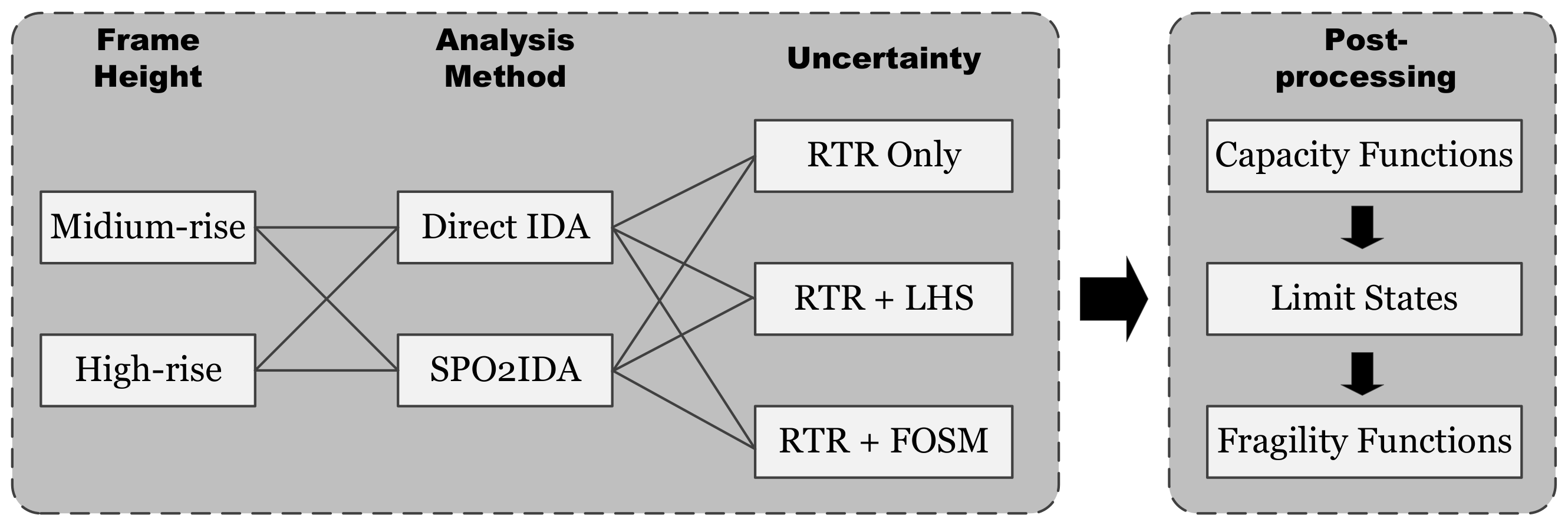
3. Procedure of Seismic Reliability Analysis

In brief, the selected frames were analyzed through IDA and POA methods. In each of the analysis processes, both FOSM and LHS reliability methods were performed. The first model is defined as a “Base Case” in which all parameters are set at their mean values. Therefore, the RTR variability is the only source of uncertainty for the Base Case. On the other hand, eight structural models were defined by the FOSM method (one model for each RV), while 25 structural models were generated based on the LHS method (25 combinations of RVs). It is noteworthy that 25 models were found to provide stable mean results from LHS-based sampling of eight RVs [7]. Using a small number of samples, e.g., ten, adversely affects the generalization of the results.

POAs are then used in the so-called SPO2IDA procedure [46]. SPO2IDA is a tool for predicting the results of IDA from POA results. For this purpose, the result of the nonlinear static POA is idealized to a multi-linear structural capacity curve and the idealized curve is converted to the ductility–strength reduction factor (${\mu }_{\mathrm{fct}}-R_{\mathrm{fct}}$) curve. SPO2IDA was first adopted by Fragiadakis and Vamvatsikos [47] for structural reliability analysis. They combined SPO2IDA with the moment-estimating technique and FOSM methods to analyze a steel frame structure.

Next, three initial points are picked to develop a curve and each section of the curve is expanded through a set of interpolations. The associated parameters are based on several IDA curves developed by Vamvatsikos through a group of 30 ground motion records as well as POA on a single degree of freedom and expanded to multi-degree of freedom systems. The results of interpolations in each part are softened and connected by the spline technique. Finally, the interpolated curves are multiplied by ductility and spectral acceleration corresponding to yield in order to generate the final summarized IDA curves. This transformation can be carried out as follows:

$$\left\{\begin{array}{c}\delta ={\mu }_{\mathrm{fct}}\times {\delta }^y\\ S_a=R_{\mathrm{fct}}\times S_a^y\end{array}\right.$$

(13)

The SPO2IDA tool results in the summarized IDA curves of $16\%$, $50\%$, and $84\%$ fractiles, and the above procedure is repeated for each of the fractiles with different coefficients. On the other hand, the direct IDA analysis is employed using 44 ground motion records, as recommended by FEMA P695 [48], in both diagonal directions and for each of the reliability assessment methods (i.e., FOSM or LHS). The results are then converted to $16\%$, $50\%$, and $84\%$ summarized curves. In POA, the created models are analyzed by nonlinear static push-over analysis and the results are directly converted to summarized IDA curves with the SPO2IDA tool. After this conversion, the same procedure as the IDA process is repeated for the pushover process. Comparing the results of LHS and FOSM methods at each of the IDA and POA types is the primary goal of this paper.

The objective of this study is to evaluate the reliability of two RC frames while accounting for both the aleatory and epistemic uncertainties. For this purpose, the probability of exceeding the limit states is evaluated according to the PEER probabilistic framework. Figure 1 illustrates a road map in this paper in which two frames are combined with two analysis methods and three uncertainties combinations to extract the capacity and fragility functions. The aleatory uncertainties are considered using the FEMA P695 ground motion set [48], and the epistemic uncertainties are selected from the moment = curvature diagram for beam and column elements. Seismic reliability analysis is performed through both the IDA and POA methods as well as two reliability analysis techniques (i.e., FOSM and LHS).

4. Case Study

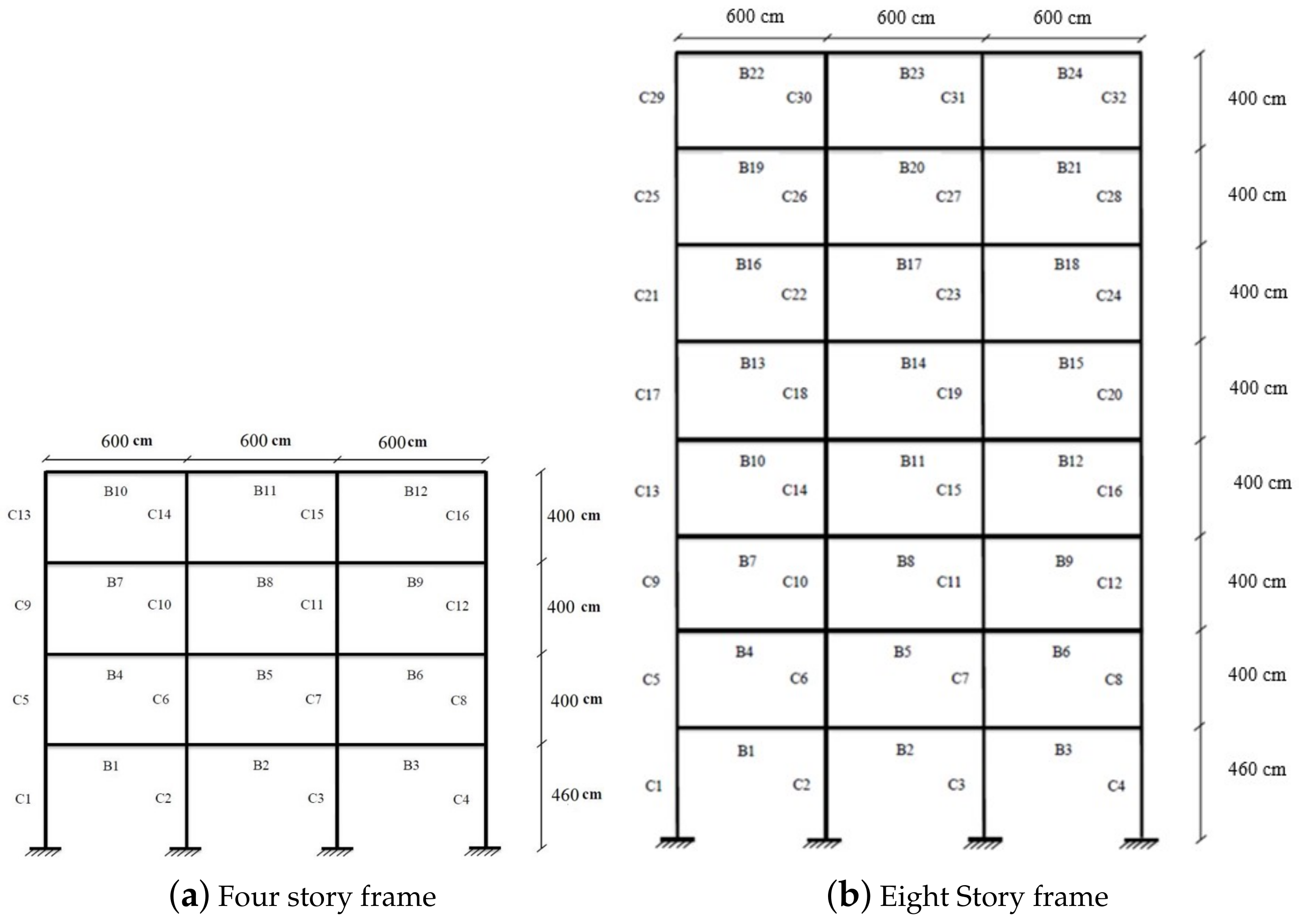
4.1. Geometry and Dimensions

To perform reliability analysis, two four-story three-bay and eight-story three-bay reinforced concrete special moment frames were chosen. The frames were originally designed by Haselton and Deierlein [13]. Figure 2 illustrates the geometry and dimension of the frames. The mechanical properties of the beam and column sections are tabulated in

Table A1. Specifications and mean values of the random variables in beam sections for four-story frame.

Elem	h [cm]	b [cm]	${\mathit{\rho }}_{\mathit{l}}$	${\mathit{\rho }}_{\mathit{l}}^{\prime }$	${\mathit{\rho }}_{\mathit{s}\mathit{h}}$	s [cm]	${\mathit{\theta }}_{{\mathit{p}}_{\mathit{b}}}$ [rad]	${\mathit{\theta }}_{{\mathit{p}\mathit{c}}_{\mathit{b}}}$ [rad]	${({\mathit{M}}_{\mathit{c}}/{\mathit{M}}_{\mathit{y}})}_{\mathit{b}}$	${\mathit{\lambda }}_{\mathit{b}}$
B1	60	55	0.0043	0.0083	0.0033	12.5	0.0414	0.1	1.21	174.15
B2	60	55	0.0043	0.0083	0.0033	12.5	0.0414	0.1	1.21	174.15
B3	60	55	0.0043	0.0083	0.0033	12.5	0.0414	0.1	1.21	174.15
B4	60	55	0.0037	0.0075	0.0033	12.5	0.0401	0.1	1.21	174.15
B5	60	55	0.0037	0.0075	0.0033	12.5	0.0401	0.1	1.21	174.15
B6	60	55	0.0037	0.0075	0.0033	12.5	0.0401	0.1	1.21	174.15
B7	60	55	0.0037	0.0075	0.0033	12.5	0.0394	0.1	1.21	174.15
B8	60	55	0.0032	0.006	0.0033	12.5	0.0394	0.1	1.21	174.15
B9	60	55	0.0032	0.006	0.0033	12.5	0.0394	0.1	1.21	174.15
B10	60	55	0.0032	0.0045	0.0033	12.5	0.0403	0.1	1.21	174.15
B11	60	55	0.0032	0.0045	0.0033	12.5	0.0403	0.1	1.21	174.15
B12	60	55	0.0032	0.0045	0.0033	12.5	0.0403	0.1	1.21	174.15

–

Table A4. Specifications and mean values of the random variables in column sections for eight-story frame.

Elem	h [cm]	b [cm]	$\mathit{\nu }$	${\mathit{\rho }}_{\mathit{tot}}$	${\mathit{\rho }}_{\mathit{sh}}$	s [cm]	${\mathit{\theta }}_{{\mathit{p}}_{\mathit{c}}}$ [rad]	${\mathit{\theta }}_{{\mathit{pc}}_{\mathit{c}}}$ [rad]	${({\mathit{M}}_{\mathit{c}}/{\mathit{M}}_{\mathit{y}})}_{\mathit{c}}$	${\mathit{\lambda }}_{\mathit{c}}$
C1	55	55	0.11	0.0115	0.0084	10	0.0631	0.1	1.187	160.59
C2	55	55	0.21	0.0105	0.0084	10	0.0503	0.1	1.173	140.88
C3	55	55	0.21	0.0105	0.0084	10	0.0503	0.1	1.173	140.88
C4	55	55	0.11	0.0115	0.0084	10	0.0631	0.1	1.187	160.59
C5	55	55	0.09	0.0115	0.0084	10	0.0655	0.1	1.19	164.85
C6	55	55	0.19	0.0105	0.0084	10	0.0521	0.1	1.176	144.62
C7	55	55	0.19	0.0105	0.0084	10	0.0521	0.1	1.176	144.62
C8	55	55	0.09	0.0115	0.0084	10	0.0655	0.1	1.19	164.85
C9	55	55	0.08	0.012	0.0084	10	0.0675	0.1	1.191	167.02
C10	55	55	0.16	0.014	0.0084	10	0.0592	0.1	1.18	150.41
C11	55	55	0.16	0.014	0.0084	10	0.0592	0.1	1.18	150.41
C12	55	55	0.08	0.012	0.0084	10	0.0675	0.1	1.191	167.02
C13	55	55	0.07	0.012	0.0084	10	0.0687	0.1	1.192	169.22
C14	55	55	0.13	0.014	0.0084	10	0.0626	0.1	1.184	156.43
C15	55	55	0.13	0.014	0.0084	10	0.0626	0.1	1.184	156.43
C16	55	55	0.07	0.012	0.0084	10	0.0687	0.1	1.192	169.22
C17	55	55	0.05	0.012	0.0084	10	0.0713	0.1	1.195	173.71
C18	55	55	0.11	0.0135	0.0084	10	0.0647	0.1	1.187	160.59
C19	55	55	0.11	0.0135	0.0084	10	0.0647	0.1	1.187	160.59
C20	55	55	0.05	0.012	0.0084	10	0.0713	0.1	1.195	173.71
C21	55	55	0.04	0.012	0.0084	10	0.0726	0.1	1.196	176
C22	55	55	0.08	0.0135	0.0084	10	0.0683	0.1	1.191	167.02
C23	55	55	0.08	0.0135	0.0084	10	0.0683	0.1	1.191	167.02
C24	55	55	0.04	0.012	0.0084	10	0.0726	0.1	1.196	176
C25	55	55	0.03	0.012	0.0084	10	0.074	0.1	1.198	178.32
C26	55	55	0.05	0.014	0.0084	10	0.0725	0.1	1.195	173.71
C27	55	55	0.05	0.014	0.0084	10	0.0725	0.1	1.195	173.71
C28	55	55	0.03	0.012	0.0084	10	0.074	0.1	1.198	178.32
C29	55	55	0.01	0.012	0.0084	10	0.0767	0.1	1.201	183.05
C30	55	55	0.03	0.014	0.0084	10	0.0752	0.1	1.198	178.32
C31	55	55	0.03	0.014	0.0084	10	0.0752	0.1	1.198	178.32
C32	55	55	0.01	0.012	0.0084	10	0.0767	0.1	1.201	183.05

(four last columns) in Appendix A. These values are, in fact, the input parameters in the predictive equations of the concrete beam-column behavior presented by Haselton et al. [11].

4.2. Constitutive Models and Random Variables

One of the crucial tasks in the nonlinear analysis is to model the frame components with multi-linear curves which demonstrate the beam and column elements’ behavior. A tri-linear backbone curve which has been previously introduced as a lumped-plasticity model by Ibarra et al. [9] is adopted in this paper. The parameters in this backbone curve can be considered as sources of epistemic uncertainties [13,39,49].

In the context of nonlinear simulations, predictive equations of modeling parameters are necessary due to the lack of sufficient experimental tests. Several equations have been proposed for steel and reinforced concrete frames [11,50]. FEMA P695 [48] represents one such constitutive model, in which the parameters of the nonlinear moment–rotation curve are a function of geometrical and structural parameters such as longitudinal and transverse reinforcement and axial and shear demand. In this research, a tri-linear backbone curve is used to model the structural elements [9]. The post-cap part of the tri-linear curve is pivotal to continued analysis up to near-collapse limit states. Hence, the precise modeling of this part, along with others, is important to achieve a reliable probability of collapse.

In this paper, four modeling parameters in the backbone curve are considered RVs. Those four RVs are applied to both beams (b) and columns (c), and thus a total of eight independent RVs are used in finite element simulations. The mean values were obtained from the predictive equations provided by FEMA P695 [48], and the related coefficient of variations (COVs) were obtained from the existing literature [3,10]. Eight RVs and the assumed COVs are listed below for the backbone curve in Figure 3a:

• COV = 0.5 for RV1: ${\lambda }_b$, and RV2: ${\lambda }_c$ ($\lambda$: cyclic deterioration capacity)
• COV = 0.1 for RV3: ${(M_c/M_y)}_b$, and RV4: ${(M_c/M_y)}_c$ ($M_c/M_y$: ratio of capping to yield moment)
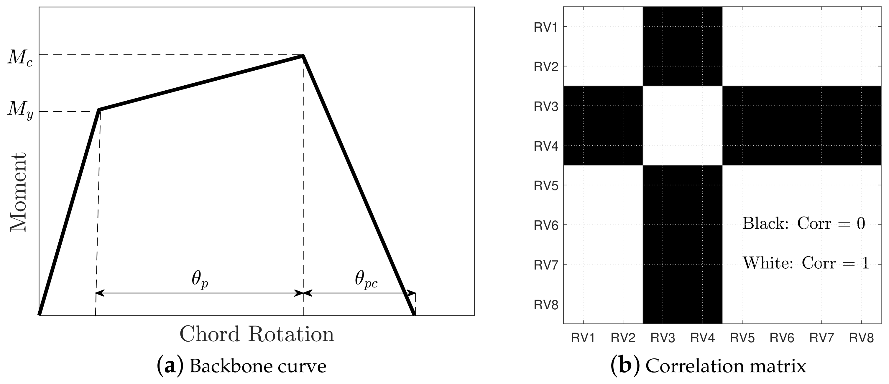
• COV = 0.6 for RV5: ${\theta }_{p_b}$, RV6: ${\theta }_{p_c}$, RV7: ${\theta }_{p{c}_b}$, and RV8: ${\theta }_{p{c}_c}$ (${\theta }_p$: plastic rotation, ${\theta }_{pc}$: post-plastic rotation)

Furthermore, a correlation matrix must be taken into account. In this paper, the RVs are either fully correlated or uncorrelated (i.e., no partial correlation is studied). Figure 3b shows the assumed correlation matrix [11], in which the fully correlated RVs have a correlation coefficient of ${\rho }_{corr}=1.0$ and are shown in white, while the uncorrelated RVs have a correlation coefficient of ${\rho }_{corr}=0.0$ and are shown in black. This matrix is basically adopted from Haselton and Deierlein [13] for RVs 1 to 6. Furthermore, we treated RV7 and RV8 (those related to ${\theta }_{pc}$) in a same way as Haselton and Deierlein [13] treated ${\theta }_p$ (for RV5 and RV6).

According to the COV values, the plastic and post-plastic rotation impose higher degrees of uncertainty on the problem in comparison to the other modeling parameters. It should be noted that the COV values of the modeling parameter are assumed to be identical for the beam and column elements. The combination of all individual uncertainty sources results in the final modeling dispersion of the fragility curves. Moreover, the modeling uncertainties are implemented in different ways for the LHS and FOSM methods. In the LHS method, the uncertainty propagation is simultaneously executed within all RVs. However, the FOSM method applies the one-at-a-time technique to propagate the uncertainty in individual RVs (i.e., creating the perturbed model) and calculates the final dispersion (error) via the closed-form equations.

By applying the predictive equations discussed before, the mean values related to each parameter can be obtained. To generate the structural models for nonlinear analysis, these values are required so that the magnitude of RVs may be changed from model to model; however, the deterministic parameters always remain in their mean values. Table A1–Table A4 (right side) illustrate the mean values of RVs for both frames.

All nonlinear transient analyses were conducted in OpenSees [51,52] using the built-in lumped plasticity models. The lumped plasticity model consists of two rotational springs at each end of the element and an elastic element in middle. The behavior of the rotational spring is generally defined as the trilinear backbone curve (see Figure 3a); its parameters can be different according to the element’s specifications. Newmark’s method was used as the integrator for dynamic analysis, while the solution algorithm was based on the Modified Newton method. In the IDA analysis, each of the 44 earthquake records was scaled based on their corresponding $S_a\left(T_1\right)$ for a 5% damping ratio. In the LHS method, a set of 25 simulations was generated for each of the studied frames. In the FOSM method, all variables were set to their mean values in the first step, and a single separate model was defined by perturbing the magnitude of an RV as a standard deviation (i.e., nine simulations). Second-order P-Delta effects were accounted for in the nonlinear analyses by setting the geometric transformation to PDelta. Both the horizontal and vertical components of the ground motion records were directly applied at the base of the finite element models. Thus, neither the spatial variability in ground motion nor the soil–structure interaction is considered [53]. The following assumptions/limitations are applied throughout the entire manuscript unless otherwise stated:

• All observations are limited to the two SMRF RC frames (four-story and eight-story) and similar frames designed according to modern design criteria.
• The epistemic uncertainty originates from four RVs, all concerning moment–rotation constitutive modeling of beams and columns, as illustrated in Figure 3a.
• There are separate assumed RVs for beam and column elements.
• The probabilistic specifications (e.g., distributional model, mean, STD, and correlation matrix) are all according to those mentioned in Section 4.2.
• All the primary results are based on a full correlation assumption among RVs. The results of fully uncorrelated models are presented in Section 5.14.
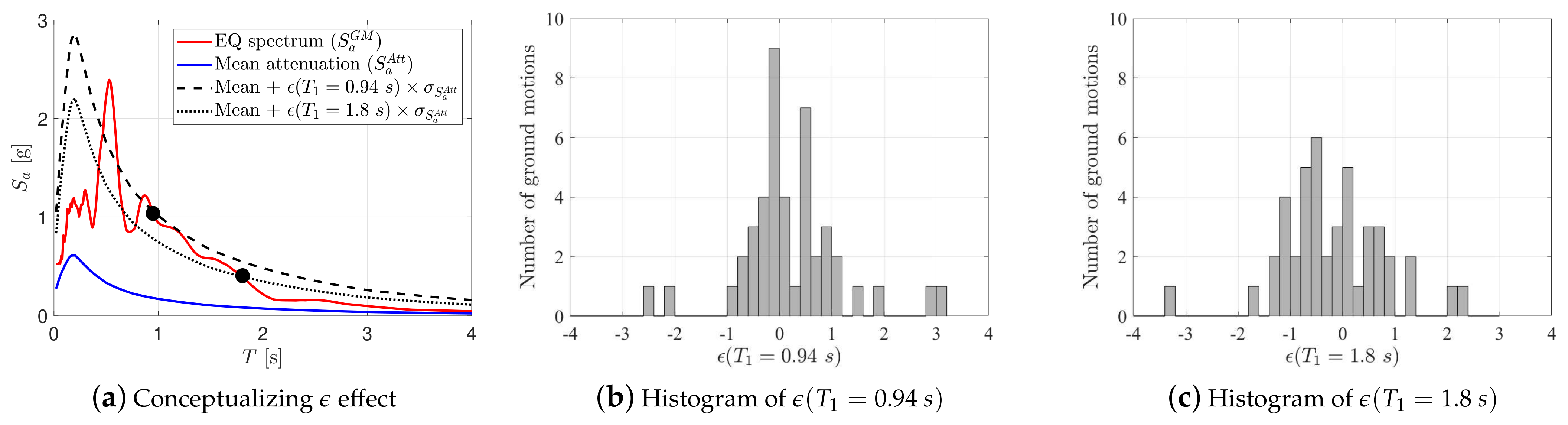
• The structural seismic responses are further modified according to the spectral shape considerations, as discussed in Section 5.1.

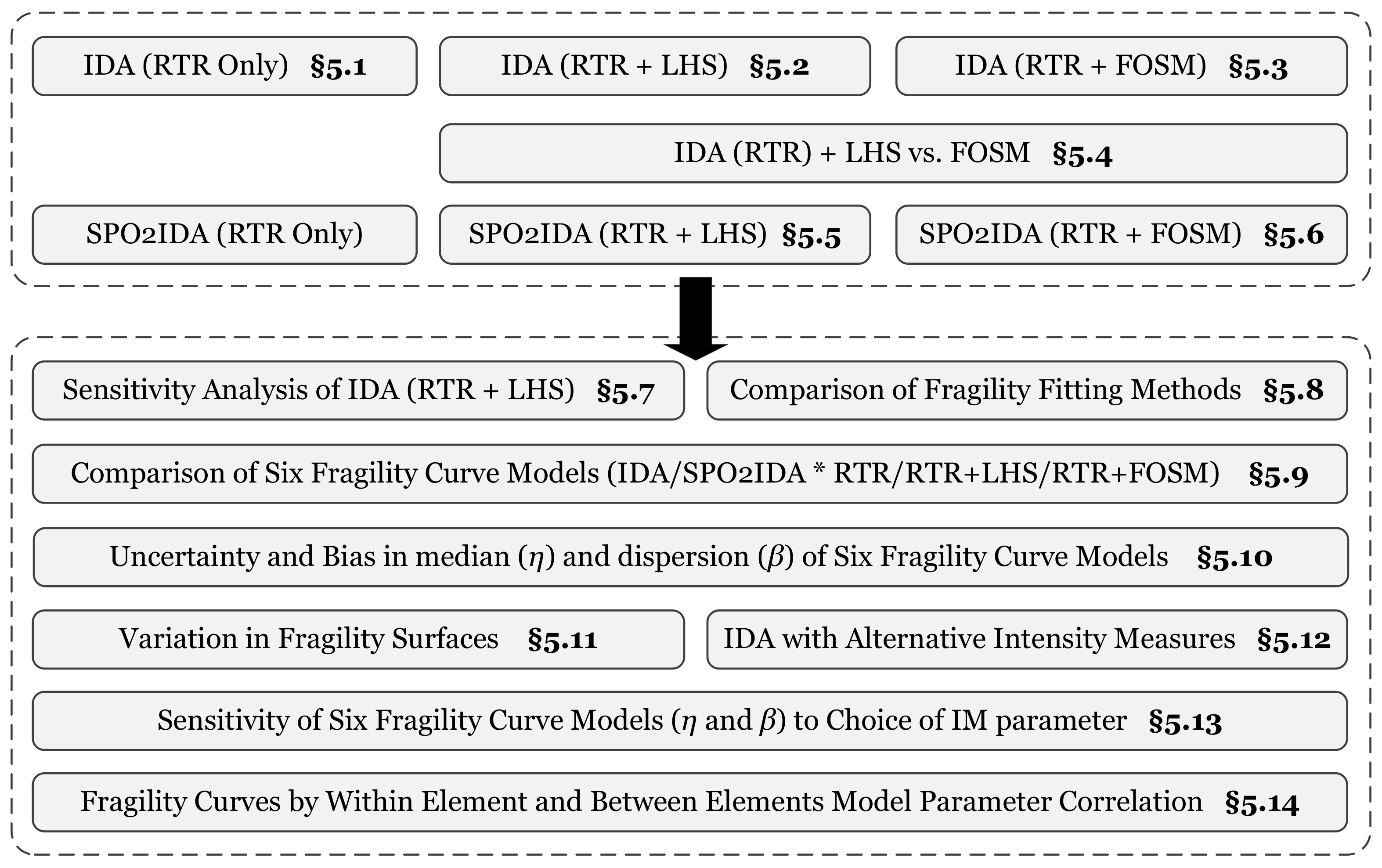
5. Results and Discussion

This paper compares different techniques and assumptions for developing seismic fragility functions. Therefore, the results are presented in fourteen subsections, each one with a separate target and outcome. Figure 4 provides a summary of all separate studies in this paper and the associated subsection number. The first six subsections discuss the variability in capacity functions in terms of summarized (i.e., 16%, 50%, and 84%) fractile curves and regions/bands. The remaining subsections are based on sensitivity and uncertainty in developing the fragility functions using the capacity functions.

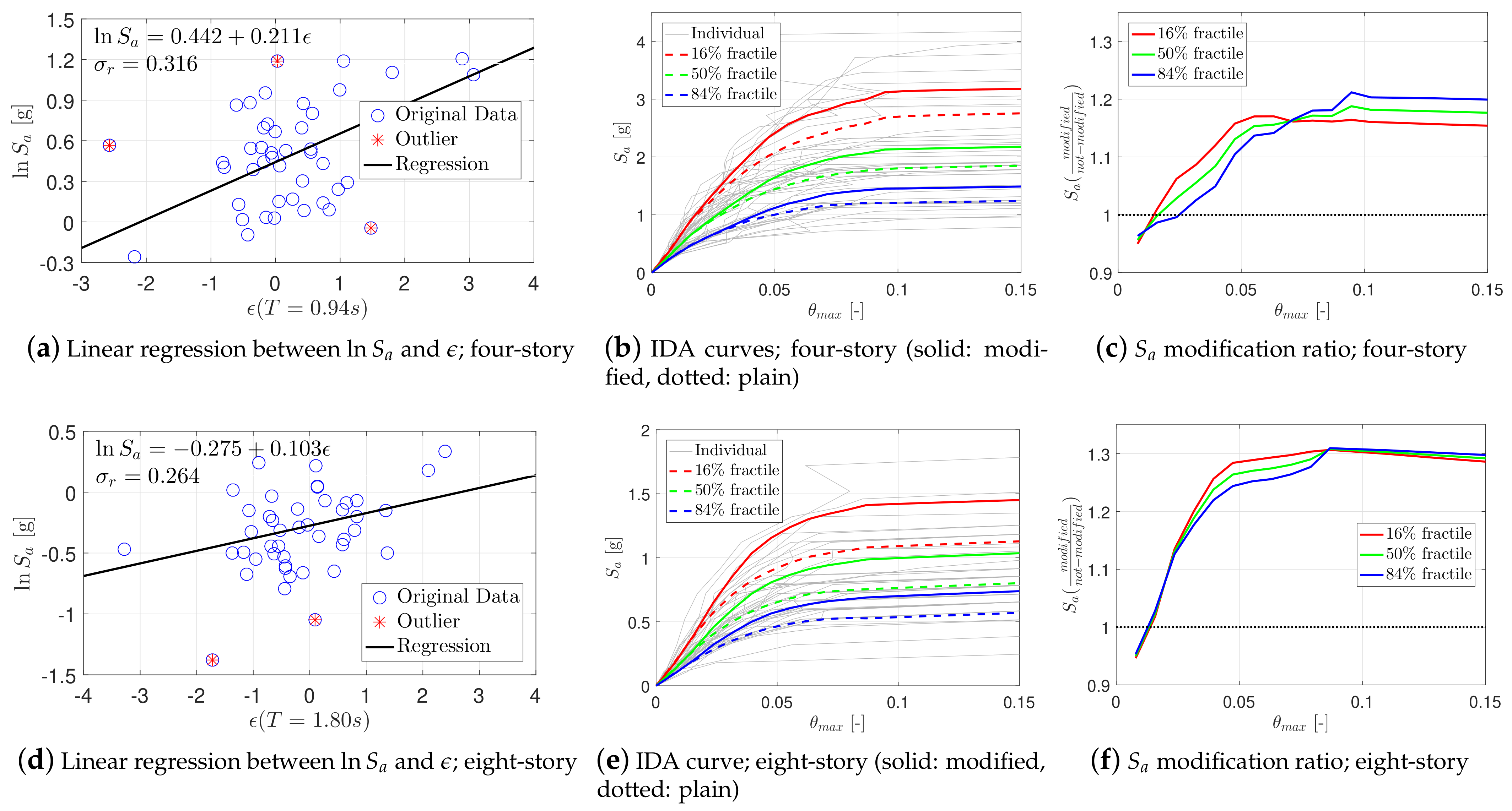
5.1. Direct IDA and Spectral Shape-Based Modifications

First, a brief review is provided about the concept of $ϵ$-based modifications for IDA median and dispersion. This discussion is mainly inspired by the pioneering work of Haselton et al. [54]. The importance of such modifications originates from the fact that selecting a suitable set of ground motions is one of the most significant steps in structural seismic performance assessment. Particularly, the inclusion of high-intensity ground motions is required to study structural collapse, while their spectral shape should be taken into account based on the $ϵ$ parameter [55]. The $ϵ$ is a multiplier of the attenuation model’s logarithmic dispersion, ${\sigma }_{S_a^{Att}}$, indicating the difference between the studied earthquake spectrum $S_a^{GM}$ and the mean predicted attenuation spectrum $S_a^{Att}$ [55]. Therefore, $ϵ$ is calculated at a specific period T as follows:

$$ϵ\left(T\right)=\frac{ln\left(S_a^{GM}\left(T\right)\right)-ln\left(S_a^{Att}\left(T\right)\right)}{{\sigma }_{S_a^{Att}}\left(T\right)}$$

(14)

The positive $ϵ$ value typically increases in the median collapse capacity [56]. One approach to selecting the ground motions is to choose those records which are consistent with the target $ϵ$-value (known as ${ϵ}_0$) depending on several factors, such as site characteristics, seismic hazard level, and the first-mode period of the structure. In this approach, the ground motion set should be altered each time based on the characteristics of the case study structure. Alternatively, Haselton et al. [54] proposed an approach that retains a generic set of ground motion records while modifying the median and dispersion of the collapse capacity results. They materialized this approach using 44 ground motions of FEMA P695 [48].

An example of $ϵ$-based spectral modification is illustrated in Figure 5a using Abrahamson and Silva [57]’s attenuation model to compute $ϵ$ and a sample record from FEMA P695. As seen in this figure, $ϵ$ is computed such that the earthquake’s spectrum crosses the dashed lines (scaled mean attenuation) at $T_1=0.94$ s for the four-story frame or $T_2=1.8$ s for the eight-story frame.

Subsequently, a linear approximation is fitted to the pair data of $ln{S}_a-ϵ$, as seen in Figure 6a,d. According to Haselton et al. [54], the modified IDA median and dispersion are calculated as follows:

$$\begin{array}{ccc}\hfill M_{mod}& =& exp\left(p_1+p_2{ϵ}_0\left(T_1\right)\right)\hfill \end{array}$$

(15)

$$\begin{array}{ccc}\hfill {\sigma }_{mod}& =& \sqrt{{\sigma }_r^2+{\left(p_2{\sigma }_{ϵ}\right)}^2}\hfill \end{array}$$

(16)

where $p_1$, $p_2$, and ${\sigma }_r$ are the intercept, slope, and residual’s dispersion of the linear regression, respectively. The ${ϵ}_0$ values are taken as ${ϵ}_0(T_1=0.94)=1.3$ and ${ϵ}_0(T_1=1.8)=1.6$ for the four-story and eight-story frames, respectively, and ${\sigma }_{ϵ}=0.35$ for both frames. These values are used assuming that the selected case studies are located at the same location as reported in [54].

Figure 5b,c illustrates the histograms of $ϵ$ values for 44 ground motions in FEMA P695 [48] at the first-mode period of the four-story and eight-story frames. It can be observed that the calculated $ϵ$ values are mostly within the range of [−1, +1]. However, the required ${ϵ}_0$ values are greater than 1.0. Therefore, performing such a modification is inevitable while using a generic set of ground motion records.

As a matter of clarification, the mean collapse capacity and the related standard deviation in all the created models are modified in both frames. Regarding the modifications mentioned above, for example, in Base Case at collapse LS, the mean and logarithmic standard deviation values of the collapse capacity for the four-story frame in the simulation method were 2.15 g and 0.38, respectively, and for the eight-story frame were 1.00 g and 0.35, respectively. According to the above amendments, it can be concluded that the median value of collapse capacity was increased by 1.17 and 1.28 times in the four-story and eight-story frames (for the Base Case) after the modification of the spectral shape effect. Similarly, this modification is applied to all maximum inter-story drift levels and all the created models to ultimately modify the IDA curve.

Figure 6b,e shows the IDA curves for the Base Case, in which only the RTR variability is considered (i.e., only 44 curves, with all other parameters in their mean value). These plots illustrate the summarized 16%, 50%, and 84% fractiles for both plain and modified spectral acceleration cases.

The ratios of the modified spectral acceleration to the plain ones are computed and plotted versus ${\theta }_{max}$ for all three summarized curves in Figure 6c,f. As can be seen, this ratio is always higher than one, and is bounded to 1.2 and 1.3 for the four-story and eight-story frames, respectively. Another interesting observation is that for the four-story frame, there is a change point (roughly about ${\theta }_{max}=0.07$) in which the trend of three fractiles is switched. While such a switch point is seen in the eight-story frame, its effect is not tangible in comparison to the four-story frame. The cause of this change can be attributed to the characteristic of the modified ground motion records. The entire modification process is based on the regression analysis, which is founded on the $ϵ$ values of the ground motions and the resulting $S_a$ values. Finally, in both frames, the trend of this ratio is nearly constant as the structures yield higher ${\theta }_{max}$ values.

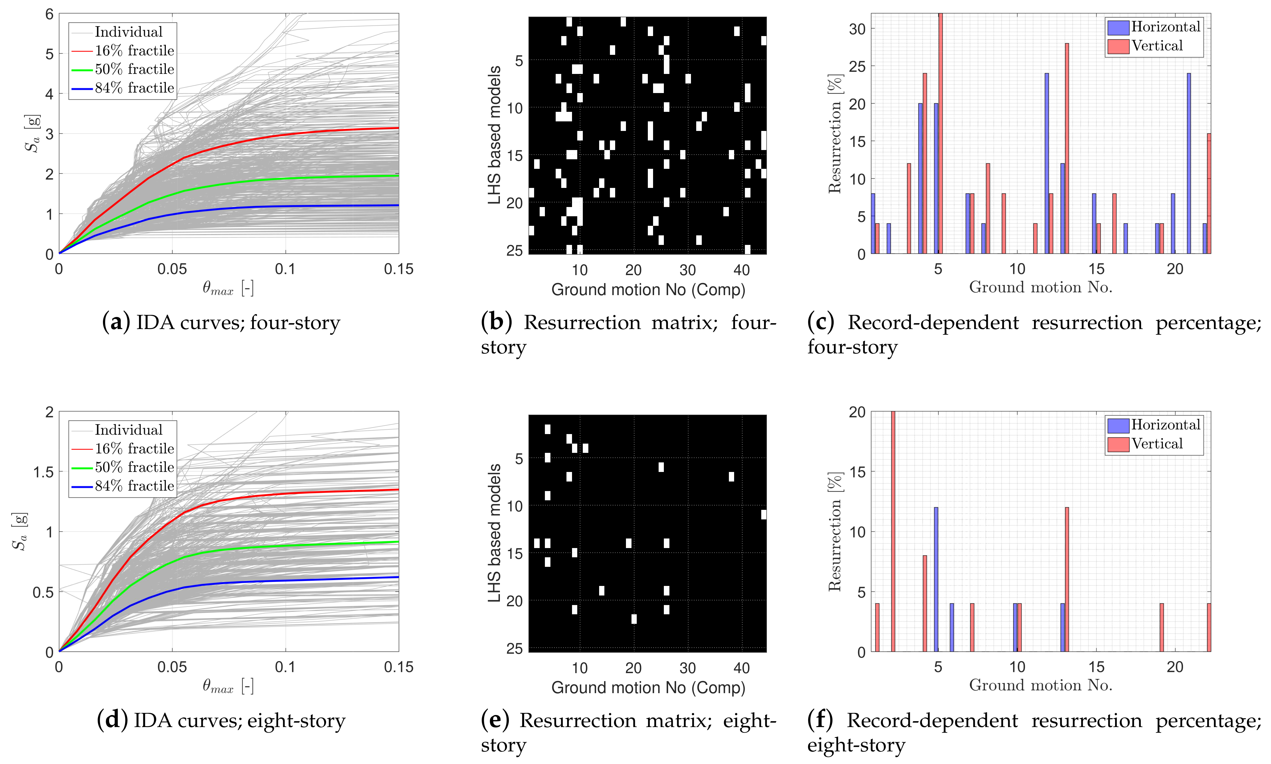
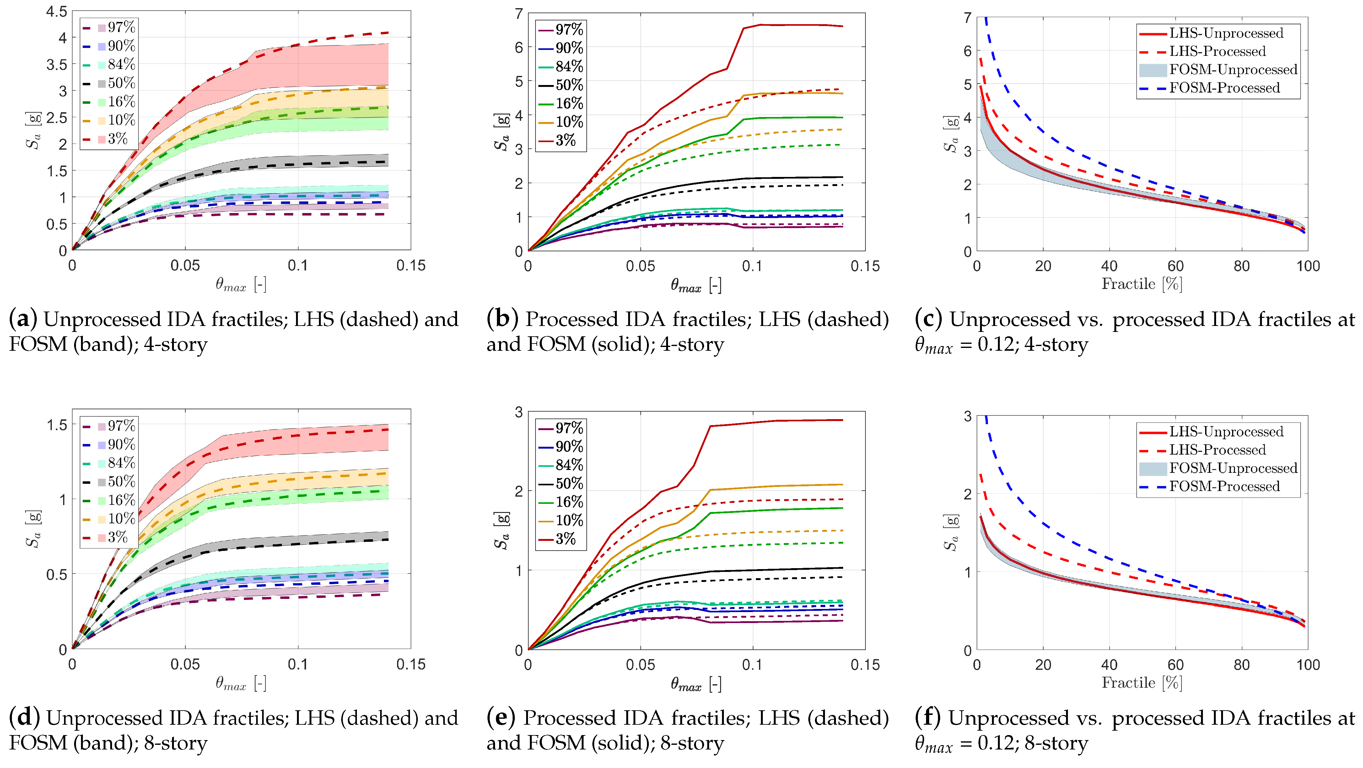
5.2. Direct IDA with LHS

This section summarizes the results of the direct IDA method combined with LHS. For each frame, a total of 44 × 25 = 1100 distinct models-records are developed. Depending on the number of required simulations to capture the collapse in each model-record, a total of 12,614 and 6592 analyses were performed for the four-story and eight-story frames, respectively. The resulting single-record IDA curves are shown in Figure 7a,d for the four-story and eight-story frames, respectively. They include the 16%, 50%, and 84% fractiles. It may be noted that the four-story frame requires larger shaking intensity compared to the eight-story one.

Focusing on the single-record IDA curves, several resurrection phenomena can be noted. This refers to a case where increasing the seismic intensity reduces the demand parameter. It is important to find out whether there is a systematic relation between the specific combination of LHS models and ground motion records. Figure 7b,e shows the binary matrix presentation of the resurrection phenomenon. The empty (white) cells correspond to resurrection. The major observations are: the number of resurrection occurrences in the four-story frame (81 simulations) is more than in the eight-story one (only 21 simulations). While no specific pattern is recognized in model-record combinations, all the resurrection cases for individual records are also plotted in Figure 7c,f separately for horizontal and vertical components. According to these figures, records #4, #5, #12, and #13 have a significant number of resurrection cases for the four-story frame, regardless of modeling uncertainty. In the case of the eight-story frame, the vertical component of records #2 and #13 and the horizontal component of record #5 cause the resurrection phenomenon. The results of this study show the affinity of the resurrection phenomenon to the inherent nature of ground motion records in conjunction with modeling specifications. The results of this section can be combined with machine learning methods to highlight the most critical combination of ground motion records and structural modeling. This is particularly useful in reliability analysis under rare failure probability events. An example of such an effort can be found in [58].

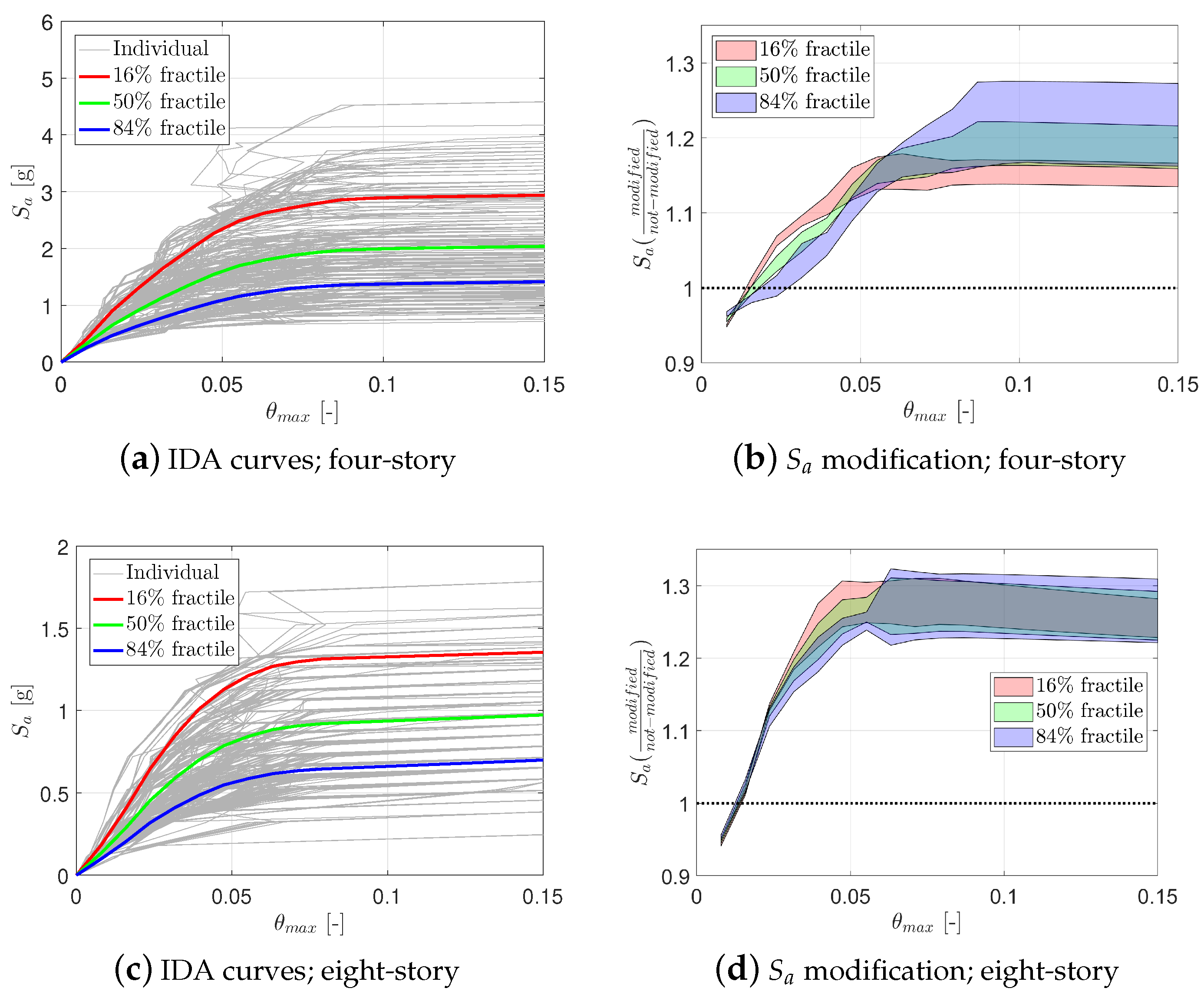
5.3. Direct IDA with FOSM

This section summarizes the results of the direct IDA method combined with FOSM. For each frame, a total of 44 × 8 = 352 distinct models-records are developed. Compared to direct IDA + LHS in Section 5.2, the computational burden is reduced by about 70%. Figure 8a,c presents all the individual IDA curves from FOSM combination and their fractiles. Compared to the LHS-based method, the curves have less dispersion.

When spectral shape-based modifications are applied to other FOSM models, a series of different ratio curves are obtained. To reduce the confusion among multiple curves, they are combined in the form of “ratio band” for three fractiles; see Figure 8b,d. Each area shows eight curves obtained from FOSM-based modeling combinations. Similar to the Base Case, the ratio bands from the eight-story frame are nearly on top of each other; however, for the four-story one, the ratio band of the 84% fractile is higher and bigger compared to the 16% and 50% fractiles.

5.4. Comparison of IDA-Based FOSM and LHS Techniques

A major aspect in comparing different techniques (FOSM vs. LHS) and assumptions (processed vs. unprocessed) in the IDA-based approach is to calculate the fractiles. One can compare different unprocessed fractile curves resulting from LHS-based and FOSM-based methods. As in the “ratio band” concept, the “fractile band” is introduced which covers the area including all eight FOSM-based IDA fractiles. For example, the 3% fractile band covers all eight individual 3% IDA fractiles related to FOSM models. The fractile bands are compared to those from LHS-based method in Figure 9a,d at seven various fractiles. While the FOSM and LHS methods are close in the central fractiles (i.e., 16%, 50%, and 84%), it is intuitive that the FOSM-based IDA fractiles are less sensitive to capturing the tails (i.e., 3%, 90%, and their counterparts), especially in the four-story frame. This can be traced back to the individual IDA curves, in which the FOSM-based IDA curves do not capture extreme events (i.e., rare events). The LHS method covers the entire space of RVs more uniformly, while the FOSM requires only two points to fit a linear approximation. This issue is less observable in the eight-story frame because of lower $S_a$ ranges.

The above-discussed assessment is founded on the fractile curves originating from the individual IDA curves, and is referred to as the “unprocessed” method. However, the final median and dispersion values are obtained by subsequent processing of these fractiles. The “processed” term herein is attributed to further treatments in the LHS and FOSM methods. In the LHS method, the processed fractiles are obtained by modification of the median and dispersion of IDAs due to the spectral shape parameter (as discussed in Section 5.1). In the FOSM-based method, the processed fractiles are obtained by both spectral shape-based modification and FOSM analytical calculation. In other words, the FOSM dispersion is calculated by modifying the fractiles of eight FOSM cases and the “Base Case” according to the spectral shape parameter. Subsequently, the deviation of median $S_a$ for each of the eight FOSM perturbed cases (with respect to the Base Case) is calculated through the FOSM linear approximation. Finally, the resulting dispersion is combined with the Base Case (RTR) dispersion using the square root of the sum of squares (Equations (2) and (3)).

The FOSM median is considered to be identical to the Base Case median (Equation (1)). With the final median and dispersion values, the respective fractiles can be obtained based on the log-normal distribution assumption of $S_a$ values. The LHS and FOSM fractiles computed based on this processed method are illustrated in Figure 9b,e. It can be observed that FOSM fractiles have larger values in comparison to the LHS method, which originates from the FOSM’s higher median and dispersion. As can be seen, processing the fractiles alters the results compared to the unprocessed assumption.

Moreover, the above four groups of fractiles (i.e., LHS-Unprocessed, LHS-Processed, FOSM-Unprocessed, amd FOSM-Processed) are compared at a deterministic ${\theta }_{max}$ of 0.12; see Figure 9c,f. The difference between the LHS-based curves originates from spectral shape-based modification. The difference between the Processed FOSM curve and the Unprocessed FOSM band originates from both spectral shape-based modification and FOSM analytical calculation.

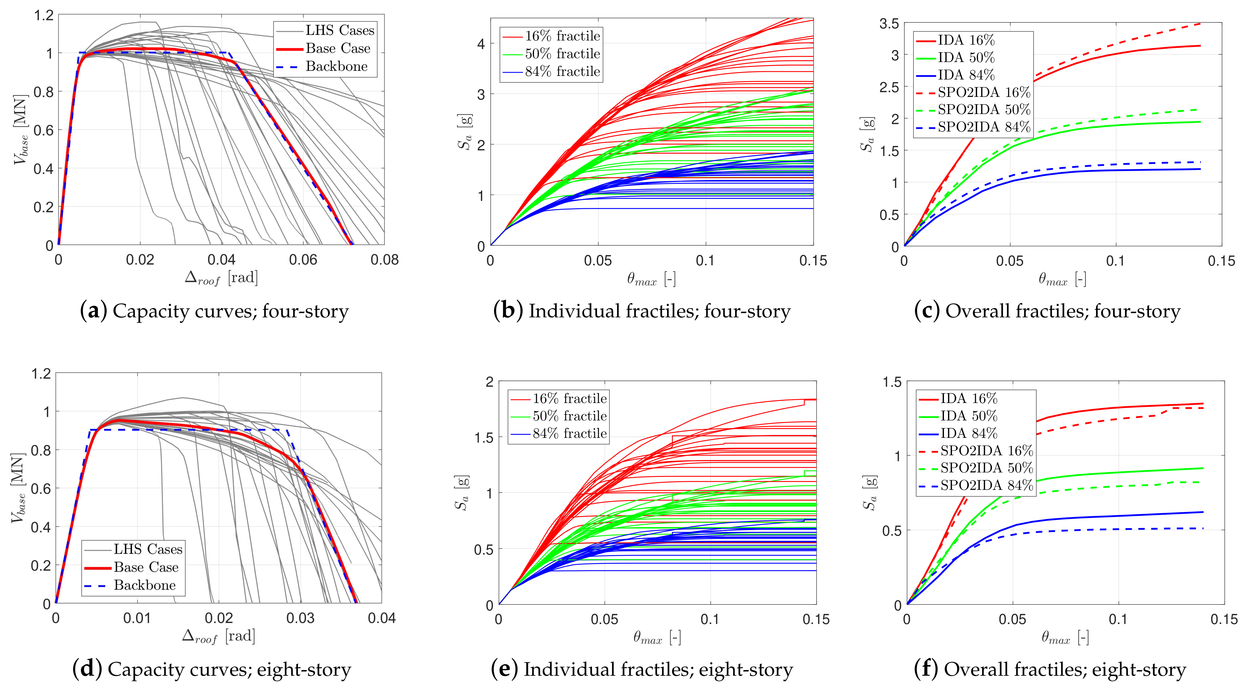
5.5. SPO2IDA with LHS

While the direct IDA method requires a relatively extensive computational effort, especially when it is combined with epistemic uncertainties, SPO2IDA offers a cost-effective alternative method to finding the approximate solution. In this section, the SPO2IDA method is combined with LHS sampling.

To use the SPO2IDA tool, the structural model should first be analyzed by nonlinear static pushover analysis. For each frame, a total of 25 pushover analyses are required. The resulting capacity curves are directly representative of diversity among the frames with modeling uncertainty. Figure 10a,d shows 25 individual LHS-based capacity curves as well as the Base Case. At the same base shear, the four-story frame has a higher roof displacement. In these plots, many capacity curves with smaller plastic rotation values can be attributed to the type of assumed distribution during modeling. Hence, this trend seems to be a logical consequence with respect to the characteristics of the log-normal distribution (i.e., higher probability density at lower variable magnitudes).

Using the results of nonlinear static pushover analyses and the SPO2IDA features, the summarized IDA curves are estimated for each of the 25 LHS models, in Figure 10b,e. As can be seen, the estimated fractiles with the SPO2IDA tool do not have natural non-uniformity (such as resurrection), similar to direct IDA.

While the estimated fractiles in the previous step are specific to each of the 25 models, they should be combined in an appropriate way to present the overall 16%, 50%, and 84% fractiles for the combined model. The calculation should be made at each ${\theta }_{max}$ level separately. The overall mean can be simply obtained by averaging the mean values of all contributing models, while the overall variance should be computed as follows:

$$\begin{array}{ccc}\hfill {\overline{\eta }}_{tot}& =& \mathrm{mean}\left({\overline{\eta }}_i\right)\hfill \end{array}$$

(17)

$$\begin{array}{ccc}\hfill Va{r}_{tot}& =& \frac{1}{N}\left(\sum _{i=1}^{N}Va{r}_i+\sum _{i=1}^N{\overline{\eta }}_i^2-N.{\overline{\eta }}_{tot}^2\right)\hfill \end{array}$$

(18)

where N is the number of models and ${\overline{\eta }}_i$ and $Va{r}_i$ are the mean and variance of each model, respectively.

Finally, the overall summarized IDA curves for SPO2IDA+LHS are shown in Figure 10c,f (dashed lines) and compared with the direct IDA + LHS results (solid lines). The differences between these two approaches are apparent. The important point is that the SPO2IDA method does not necessarily underestimate or overestimate the results of direct IDA. While SPO2IDA overestimates the summarized IDA curves in the four-story frame, it underestimates them in the eight-story one.

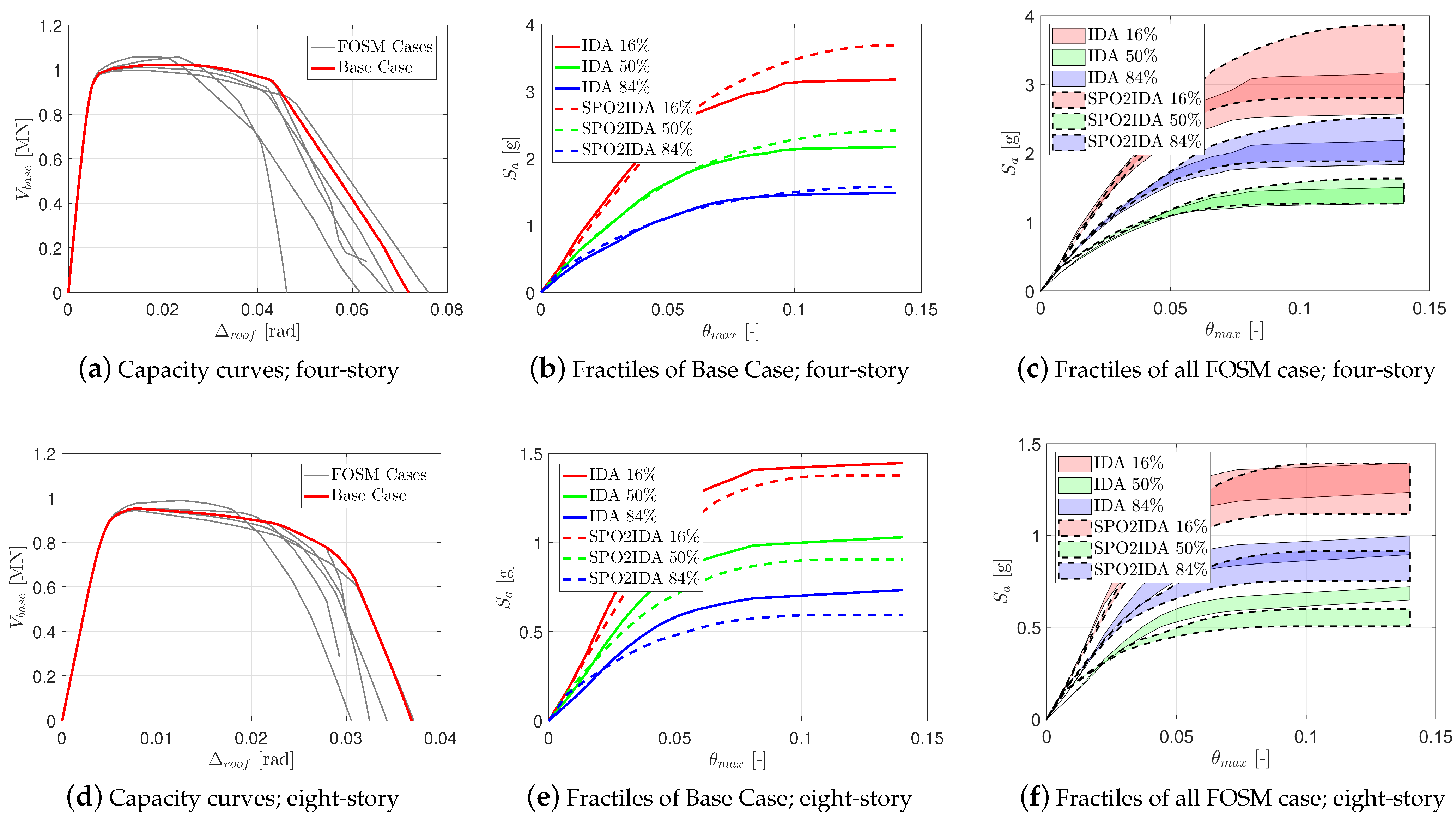
5.6. SPO2IDA with FOSM

This last set of simulations combines the approximate SPO2IDA method with realizations from FOSM, and performs only eight nonlinear static pushover analyses. Figure 11a,d presents the individual capacity curves. It is noteworthy that RVs 1 and 2 do not affect the capacity curve because the energy dissipation capacity is a parameter with respect to the cyclic loading, and is not considered in the static pushover analysis.

Figure 11b,e compares the summarized IDA curves based on SPO2IDA and direct IDA methods for the Base Case. These two plots could be presented in a separate subsection; however, we integrated them into this figure to save space. Again, the tendency of SPO2IDA to overestimate the four-story frame and underestimate the eight-story one is intuitive.

Finally, Figure 11c,f compares eight other FOSM-based models based on SPO2IDA and direct IDA methods. The results are presented in the form of uncertainty regions rather than multiple curves, which may confuse the reader. According to these figures, the SPO2IDA approach leads to larger uncertainty for the same models analyzed by the direct IDA method. The general trend of over- and underestimation of the results is similar to the Base Case.

5.7. Limit States and Sensitivity

Thus far, all the capacity curves with different analysis techniques and various assumptions for the uncertainty sources have been discussed in the previous subsections. The transition step from capacity curves to fragility functions is LS values. Because this paper is mainly focused on collapse fragility curves, we define the collapse point (or global instability) where the capacity curve is flattening.

Only for the capacity curves presented in Section 5.2 (which is thus far the most comprehensive method in our database) have we identified these IM capacity points $I{M}^c$. Figure 12a,b presents two matrices showing the $I{M}^c$ for the four-story and eight-story frames, respectively. Each cell in this matrix presents the capacity IM (which corresponds to the failure point) for a particular combination of ground motion record and modeling sampling. Larger IM capacity values show a higher capacity of that particular combination against failure. For example, in the case of the four-story frame, ground motions 1 to 6 lead to a generally higher $I{M}^c$ value. This means that the structure requires a higher $S_a\left(T_1\right)$ value at the time of failure (and probably will require more scaling steps during IDA).

Another important aspect is the height of the structure. Figure 12c shows the ratio of collapse $S_a$ from four-story to eight-story models. As can be seen, there is large variability, from 0.5 to 5.5. This means that an impact of a model-record combination is structure-dependent. While in the majority of cases the required $I{M}^c$ for the four-story frame is higher, in a few combinations the eight-story frame has a higher capacity.

Next, the sensitivity of collapse capacities is computed with respect to eight input RVs. The linear correlation is the simplest method to evaluate the sensitivity, and is mainly appropriate for RVs which have a linear dependency. Let us assume that for a sampling of the input random vector $\mathcal{X}=\left\{{\mathit{x}}^{\left(1\right)},{\mathit{x}}^{\left(2\right)},\dots ,{\mathit{x}}^{\left(N\right)}\right\}$, the corresponding model response is $\mathcal{Y}=\left\{y^{\left(1\right)},y^{\left(2\right)},\dots ,y^{\left(N\right)}\right\}$. The input–output (I-O) correlation is computed using a linear correlation coefficient between the ith input and the output:

$${\rho }_{I-O}^i\stackrel{\mathrm{def}}{=}\rho \left(X_i,Y\right)=\frac{\mathbb{E}\left[\left(X_i-{\mu }_i\right)\left(Y-{\mu }_Y\right)\right]}{{\sigma }_i{\sigma }_Y}$$

(19)

where ${\mu }_i\stackrel{\mathrm{def}}{=}\mathbb{E}\left[X_i\right]$, ${\mu }_Y\stackrel{\mathrm{def}}{=}\mathbb{E}\left[Y\right]$, and ${\sigma }_i$ and ${\sigma }_Y$ are the standard deviations.

To evaluate the sensitivity of collapse capacity points, each column in Figure 12a (or Figure 12b) is assumed to be $y^{\left(i\right)}$ (a vector of $25\times 1$), while $\mathcal{X}$ is the $25\times 8$ matrix of LHS-based input RVs. This means that sensitivity indices are computed separately for each ground motion record. For a particular ground motion record, the sensitivity indices are recorded in a $8\times 1$ vector, while the results of all ground motions are recorded in a $8\times 44$ matrix; see Figure 12d,e. According to these figures, the impact of input RVs on the collapse capacity of four-story and eight-story frames is different. For the four-story frame, RV3 and RV4 are the least sensitive variables, while all other six RVs have a much higher sensitivity index. In the case of the eight-story frame, again RV3 and RV4 have minimum sensitivity index; however, depending on the inherent characteristics of the ground motion, the sensitivity matrix can be very heterogeneous. For model reduction purposes, RV3 and RV4 can be removed from the epistemic uncertainties list in the four-story frame, while it is recommended to keep all eight RVs in the case of the eight-story frame. Furthermore, it seems that a combination of different modeling uncertainties with ground motion records has a completely different local impact on the structural system, as can be seen in multiple plots of Figure 12.

Later, in Section 5.10, four different LSs are used to compare various fragility functions. There have been different definitions proposed for ${\theta }_{max}$-based limit states in the literature. Therefore, to avoid confusion with other papers and to skip the complexities associated with labeling, we directly connect four limit states with ${\theta }_{max}$ values. These four limit states are: LS1 (${\theta }_{max}$ = 0.02), LS2 (${\theta }_{max}$ = 0.04), LS3 (${\theta }_{max}$ = 0.10), and LS4 (${\theta }_{max}$ = 0.12).

5.8. Uncertainty in Fragility Functions: Fitting and Randomness

With all the capacity functions, we are now able to to derive the collapse fragility functions. In this section, the impact of various assumptions in fragility curve derivation is investigated and the corresponding uncertainty is quantified.

In Section 5.1, we discussed the importance of spectral acceleration modifications and applied them to capacity curves; see for example Figure 6b. Similarly, this modification can be propagated into fragility functions. Figure 13a,g illustrates two examples for the RTR only and RTR + LHS models. Recall from capacity functions that spectral acceleration modification increased the capacity IM at the collapse level. Therefore, the probability of LS exceedance (in this case collapse) is reduced under the $S_a$ modification. This works in favor of the structure.

As discussed in Section 2.2, a fragility function is in fact a logarithmic CDF fitted to the discrete data points. Several techniques can be used for this curve fitting. Figure 13b,h compares four logarithmic CDF models fitted to four-story and eight-story frames. These figures show the empirical CDF curves. Data are fitted into RTR-only models. For any practical purposes, there is a negligible (if any) difference among the fragility models. Thus, one may ignore the uncertainties associated with the fragility function fitting in this type of RC frame. This finding is limited to the current paper, and may not be true in general [59].

It is interesting to compare the individual fragility curves from 25 LHS models (each one using 44 ground motions) with the overall combined model (using 1100 simulations). Figure 13c,i shows such a comparison. As can be seen, there is large variation among the fragility curves. Furthermore, it is important to determine any potential relationship between the median and dispersion of fragility curves from LHS models. Figure 13d,j presents such relations. While the median increases, dispersion does not follow a specific trend. However, it varies 0.42 ± 0.04 for the four-story frame and 0.34 ± 0.04 for the eight-story one. These numbers are consistent with FEMA P695 [48] recommendations.

Baker [27] proposed a method to effectively collect structural analysis data for fragility function fitting. This method essentially has four steps: (1) determine the $\eta$ and $\beta$ values of the fragility function (Equation (8)); (2) collect data via MCS by generating collapses or non-collapses at different IM levels according to the collapse probability from the previous step; (3) estimate a fragility function using data from the previous step; (4) repeat steps 2 and 3 N times to measure how similar the estimated fragility functions are to the original one. Figure 13e,k shows over 100 fragility functions generated in this way and then compared to the original one for the RTR + LHS case.

Last but not least, Figure 13f,l presents the concept of robust fragility [60]. This concept defines a prescribed confidence interval for the estimated fragility curve. The Robust Fragility is defined as the expected value for a prescribed fragility model considering the joint probability distribution for model parameters $\mathbf{X}$. Using the Total Probability Theorem, the robust Fragility can be written as [29]

$$\mathbb{P}\left[\mathrm{C}|\mathrm{IM}=I{M}_i,\mathbf{D}\right]={\int }_{{\mathrm{\Omega }}_X}\mathbb{P}\left[\mathrm{C}|\mathrm{IM}=I{M}_i,\mathbf{X}\right]f\left(\mathbf{X}|\mathbf{D}\right)d\mathbf{X}$$

(20)

where $\mathbf{X}$ is the vector of fragility model parameters (i.e., $\eta$ and $\beta$), ${\Omega }_X$ is its domain, and $f\left(\mathbf{X}|\mathbf{D}\right)$ is the joint probability distribution for fragility model parameters given the vector of data $\mathbf{D}$.

The variance of Equation (20) forms the ± one standard deviation for the fragility curves (i.e., the confidence interval) [60] presented in Figure 13f,l.

5.9. Uncertainty in Fragility Functions: Models

This section focuses on a combination of various analysis techniques and uncertainty sources, as discussed in Figure 1, on the developed fragility curves. Figure 14a,d compares the fragility curves from the direct IDA and SPO2IDA methods combined with only RTR variability and RTR + LHS. Four different fragility curves are obtained, showing the impact of both the modeling uncertainty and analysis technique. The main observation is that adding the LHS-based modeling uncertainty mainly affects the median value (ie.e, it shifts the curve to the left) and slightly increases the dispersion. However, comparing the direct IDA and SPO2IDA methods reveals different behavior in the four-story and eight-story frames. While the SPO2IDA tries to increase the median values in the four-story frame, it reduces them in the eight-story one. In addition, it seems that the SPO2IDA-based curves in the four-story frame are the rotated version of the direct IDA method around the heel, while in the eight-story frame the SPO2IDA-based curves are a simple translation of direct IDA curves.

Figure 14b,e compares three fragility curves solely based on the direct IDA method. According to these figures, the inclusion of LHS-based modeling uncertainties in the seismic reliability analysis reduces the median collapse capacity. It can be noted that the FOSM-based method, which is based on a linear approximation of the structural response regarding RVs, is herein applied to the semi-logarithmic space because of the exponential relationship between the structural response and RVs. Therefore, the FOSM-based method cannot alter the median, and merely modifies the standard deviation. Comparing the LHS and FOSM-based methods reveals that, due to the inclusion of modeling uncertainties, the amount of their impact on the fragility functions depends on the range of intensity measure $S_a$. This can be attributed to the different assumptions and simplifications underlying each reliability method. This in turn implies that utilizing a proper method for fragility assessment, along with a suitable hazard analysis, is crucial to attaining the correct probability of collapse. The results presented herein are valid for the case study frames.

A similar comparison can be made for SPO2IDA-based methods; see Figure 14c,f. The impact of LHS-based modeling uncertainty is higher compared to the FOSM-based approach. It is noteworthy that if the studied RVs are related to the dynamic properties of the structure, the application of the SPO2IDA is not recommended, as this method is entirely based on nonlinear static analysis.

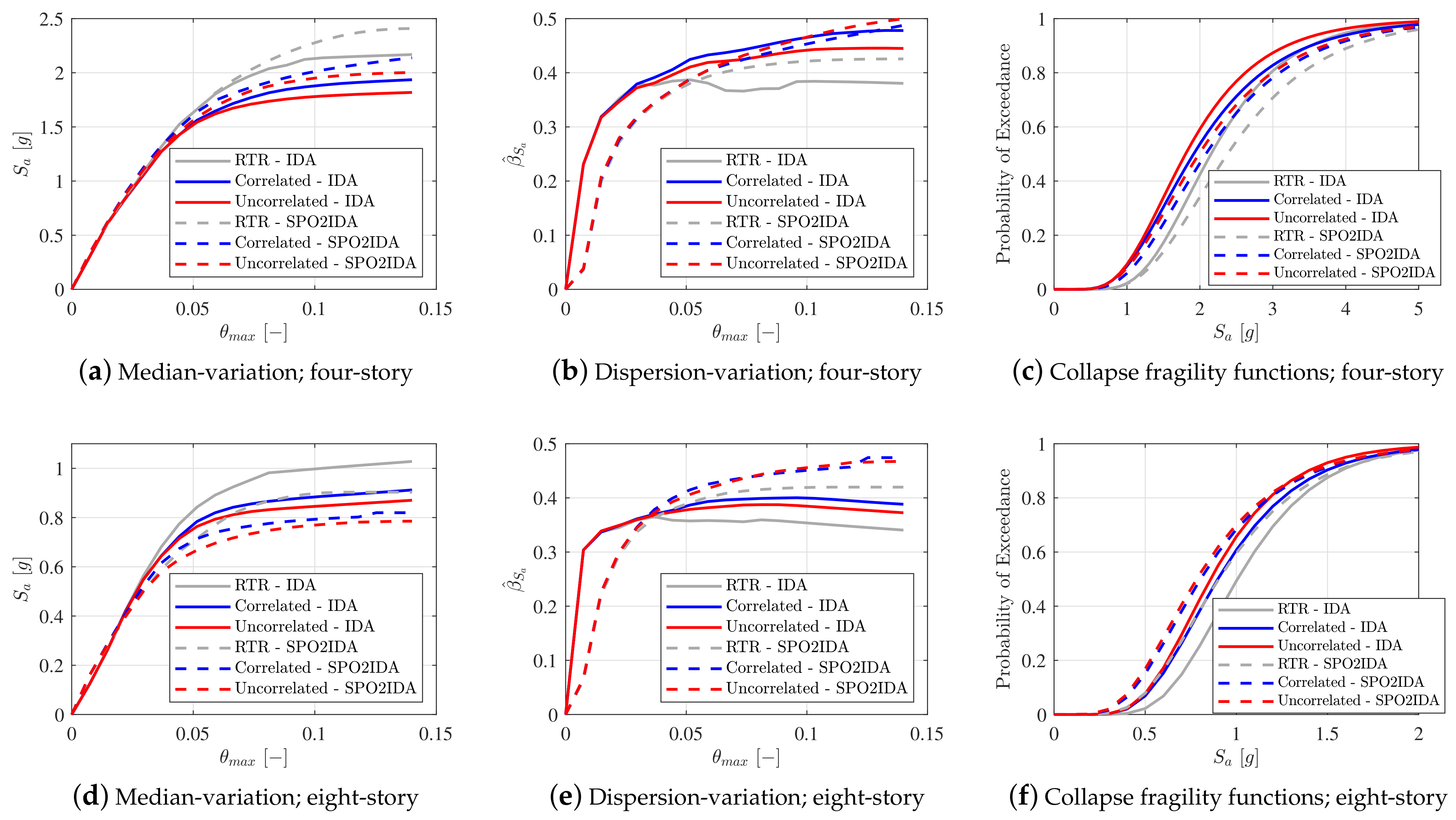
5.10. ${\theta }_{max}$-Dependent Median and Dispersion

Thus far, all the presented results have been based on collapse LS. In this section, the dependency of the median and dispersion values on ${\theta }_{max}$ is investigated. In addition, this study reveals the thresholds at which the impact of modeling uncertainties begin to diverge. Figure 15a,d presents the median IDA curves for two analysis techniques combined with two reliability methods; note again that the median of RTR and RTR+FOSM cases are identical, as FOSM is not able to change the median. These curves are later used as $\eta$ parameters in developing fragility functions. The major observations are:

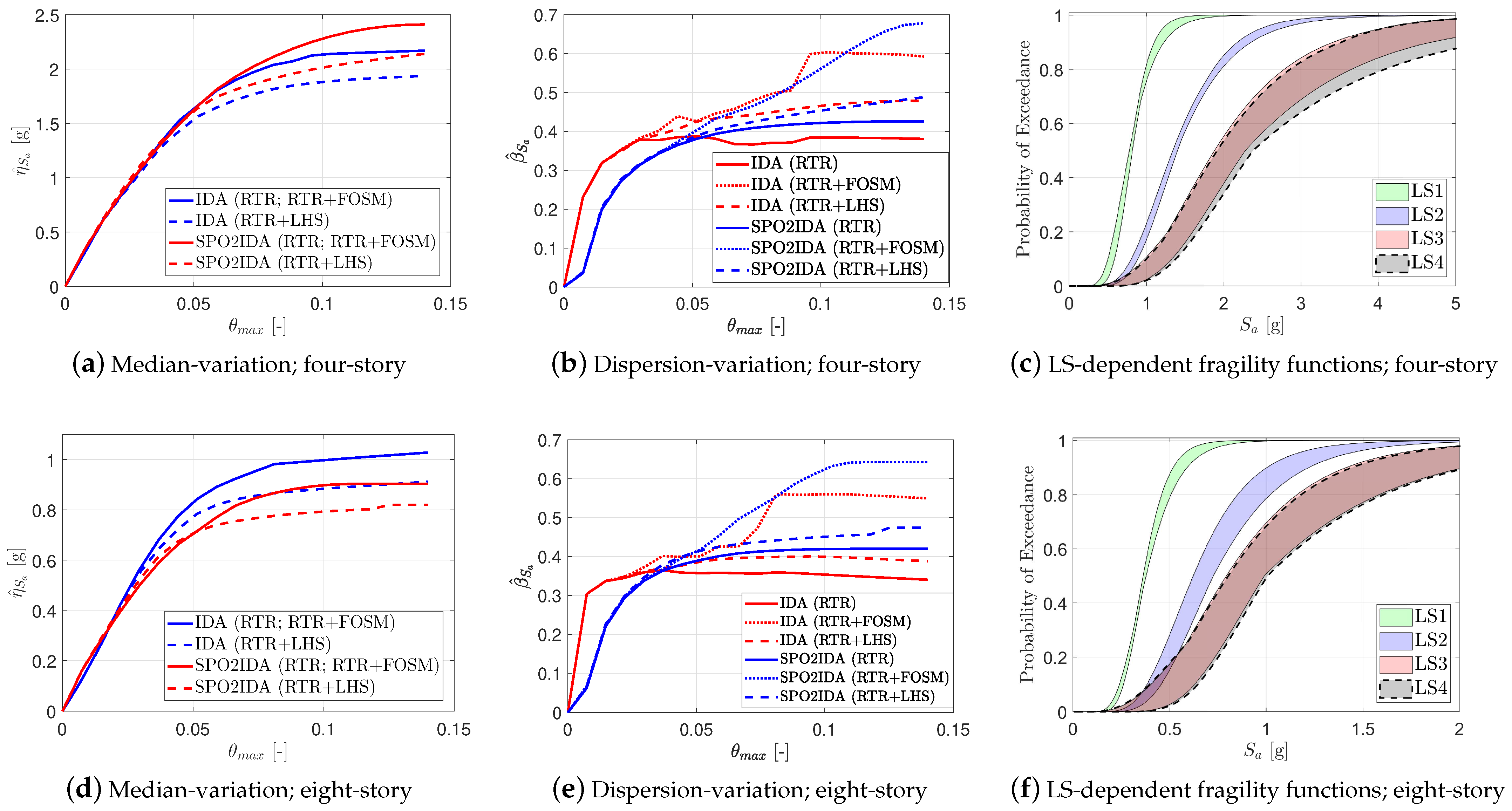
• The median curves start diverging at approximately ${\theta }_{max}$ = 0.04 and 0.02 for four-story and eight-story frames, respectively.
• Comparing direct IDA methods, in both frames the RTR-only model (as well as the FOSM-based method) yields a higher median than the LHS-based one.
• Comparing SPO2IDA methods, in general, they are similar to the direct IDA method; however, for a small range of ${\theta }_{max}$ (i.e., 0.03–0.04), the LHS-based method has a slightly higher median.
• Comparing FOSM-based (or RTR only) methods, in the four-story frame SPO2IDA leads to a higher median, while in the eight-story one it is vice versa.
• Comparing LHS-based methods leads to similar conclusions as for the FOSM-based (or RTR only) method.
• Overall, the FOSM-based method does not affect the median, and the LHS-based method reduces the median (i.e., the inclusion of modeling uncertainty reduces the median of fragility functions).

Figure 15b,e presents the dispersion of fragility functions. Again, the previously discussed six combinations are compared. The major observations are:

• The direct IDA and SPO2IDA methods have two different trends at the lower ${\theta }_{max}$ values, in contrast with median response.
• Comparing direct IDA methods, both the LHS-based and FOSM-based approaches increase the $\beta$ value compared to the RTR-only method. This augmentation in dispersion is consistent with involving additional modeling uncertainties in the problem.
• Comparing SPO2IDA methods, the inclusion of modeling uncertainties increases the composite dispersion; however, the impact of FOSM is much greate than the LHS-based approach.
• Comparing FOSM-based methods, this method always leads to higher $\beta$ compared to the LHS-based approach and RTR-only model.
• Comparing LHS-based methods, the LHS-based $\beta$ values for direct IDA are higher than the SPO2IDA method in the four-story frame, and the trend is vice versa in the eight-story frame after ${\theta }_{max}$ of 0.04.
• Overall, the combination of these six cases yields a relatively large uncertainty in the $\beta$ value. This uncertainty, which increases with ${\theta }_{max}$, is about 0.35 to 0.65 in both frames.

Table 1. Uncertainty in dispersion values from different simulation strategies, different frames, and limit states. The red and blue cells are associated with ratios greater and less than one, respectively.

	${\mathit{\beta }}_{\mathit{i}}$				${\mathit{\beta }}_{\mathit{i}}/{\mathit{\beta }}_{\mathbf{IDA}-\mathbf{RTR}}$
Simulation Strategy	LS1	LS2	LS3	LS4	LS1	LS2	LS3	LS4
4S; IDA (RTR)	0.34	0.38	0.38	0.38	1.00	1.00	1.00	1.00
4S; IDA (RTR+FOSM)	0.34	0.42	0.60	0.60	1.00	1.11	1.58	1.58
4S; IDA (RTR+LHS)	0.34	0.4	0.47	0.48	1.00	1.05	1.24	1.26
4S; SPO2IDA (RTR)	0.25	0.35	0.42	0.42	0.74	0.92	1.11	1.11
4S; SPO2IDA (RTR+FOSM)	0.25	0.36	0.56	0.64	0.74	0.95	1.47	1.68
4S; SPO2IDA (RTR+LHS)	0.25	0.36	0.45	0.47	0.74	0.95	1.18	1.24
8S; IDA (RTR)	0.34	0.36	0.35	0.34	1.00	1.00	1.00	1.00
8S; IDA (RTR+FOSM)	0.34	0.4	0.56	0.56	1.00	1.11	1.60	1.65
8S; IDA (RTR+LHS)	0.34	0.37	0.4	0.39	1.00	1.03	1.14	1.15
8S; SPO2IDA (RTR)	0.27	0.37	0.42	0.42	0.79	1.03	1.20	1.24
8S; SPO2IDA (RTR+FOSM)	0.28	0.38	0.62	0.64	0.82	1.06	1.77	1.88
8S; SPO2IDA (RTR+LHS)	0.28	0.39	0.45	0.46	0.82	1.08	1.29	1.35

reports the dispersion results from different simulation strategies at different limit state values for both four-story and eight-story frames. The absolute dispersion values ${\beta }_i$, as well as their normalized value based on the reference model, i.e., IDA (RTR), are provided. As can be seen, the range of dispersion values increases with the limit state. For LS1, $\beta \in$ [0.25–0.34] and [0.27–0.34] for the four-story and eight-story frames, respectively. For LS4 (i.e., collapse limit state), $\beta \in$ [0.38–0.60] and [0.34–0.64] for the four-story and eight-story frames, respectively. According to Table 1, using the simplified SPO2IDA method instead of IDA drops the $\beta$ value by 20–25% for LS1, while the dispersion increases by about 11–24% for LS3 and LS4. In the case of LS2, the dispersion is reduced by up to 8% for the four-story frame, while the ratio increases by up to 3% for the eight-story frame. Therefore, using the simplified SPO2IDA technique may decrease or increase the dispersion by up to 25% depending on the limit state. Combining the modeling uncertainties with RTR variability (from IDA) increases the dispersion values by 5–26% and 3–15% when using the direct LHS sampling for the four-story and eight-story frames, respectively. However, the dispersion increases by 11–58% and 11–65%, respectively, when using the FOSM algorithm. Therefore, using the simple reliability analysis technique instead of direct LHS sampling increases the dispersion twofold. Combining the RTR variability with modeling randomness from the SPO2IDA method provides a similar qualitative observation as that of the IDA method. However, using the SPO2IDA method instead of IDA underestimates the combined RTR modeling dispersion.

By combining the median and dispersion values from the previous Figure 15a,b,d,e and defining four LSs, it is possible to derive six fragility curves for each LS. These four LSs have been already defined in Section 5.7, and here are tagged from LS1 to LS4. In order to reduce the confusion among ($4\times 6=24$) fragility curves, the so-called “uncertain fragility region” is shown in Figure 15c,f for four LSs. The uncertainty fragility region is developed by taking the minimum and maximum of all six fragility curves at any desired $S_a$ value. Increasing the LS level increases the thickness of the uncertain fragility region and rotates it even more. This means that proper use of an analysis technique and reliability-based method is critical at higher LSs.

5.11. Fragility Surfaces

Finally, the combination of two $\eta$ and three $\beta$ (with no specific LS value) yields six fragility surfaces [61]. The contour plot version of those fragility surfaces for the four-story frame is shown in Figure 16a. Any point on the surface is the exceedance probability of a particular combination of $<{\theta }_{max},S_a>$, analysis technique, and reliability method. Comparing these six models, all are different, especially around the tail (i.e., when the ${\theta }_{max}$ approaches large values). These plots can be interpreted from a reliability viewpoint as well; the extent of the “safe” area in the 2D contour plots (in which the probability of exceedance of any desired combination of $<{\theta }_{max},S_a>$ is zero). These reliability-based plots are shown in Figure 16b, where the white represents safety and black is failure. Safety/failure is based on binary classification of the continuous probability of exceedance with the threshold of 0.01 (a practically small enough value in structural engineering).

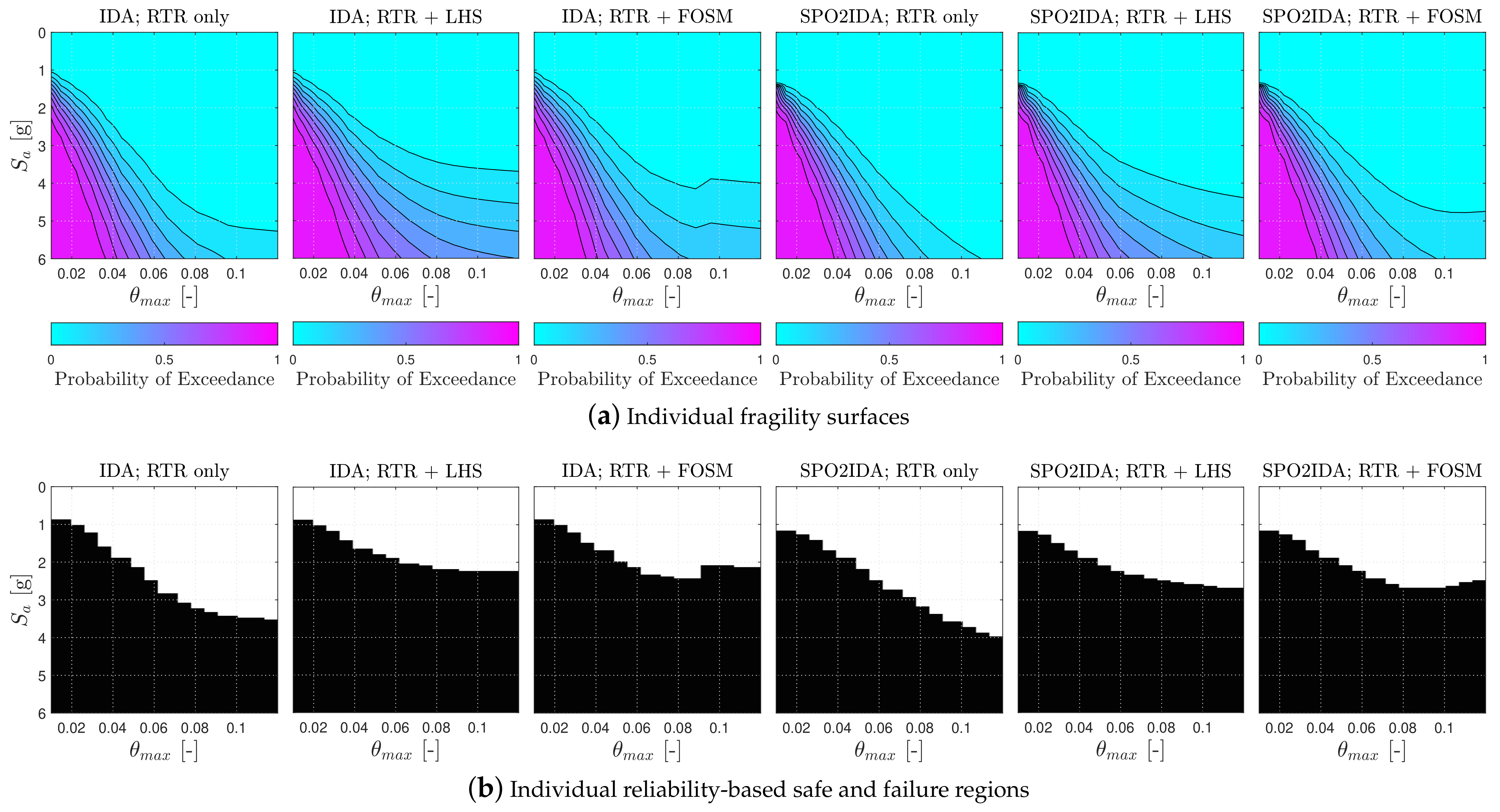
• The reliability-based failure probability can be simplified to $p_f={\int }_{S_a}{\int }_{{\theta }_{max}}\mathbb{P}\left[S_a,{\theta }_{max}\right]\ge 0.01$.
• For the IDA based method, $p_f$ is 63% (IDA only), 78% (LHS), and 77% (FOSM).
• For the SPO2IDA based method, $p_f$ is 60% (IDA only), 71% (LHS), and 72% (FOSM).
• Again, the inclusion of epistemic uncertainty increases failure by about 15% and 10% in the IDA-based and SPO2IDA-based methods, respectively.
• Depending on the type of analysis and uncertainty propagation, failure may vary from 71% to 78%.

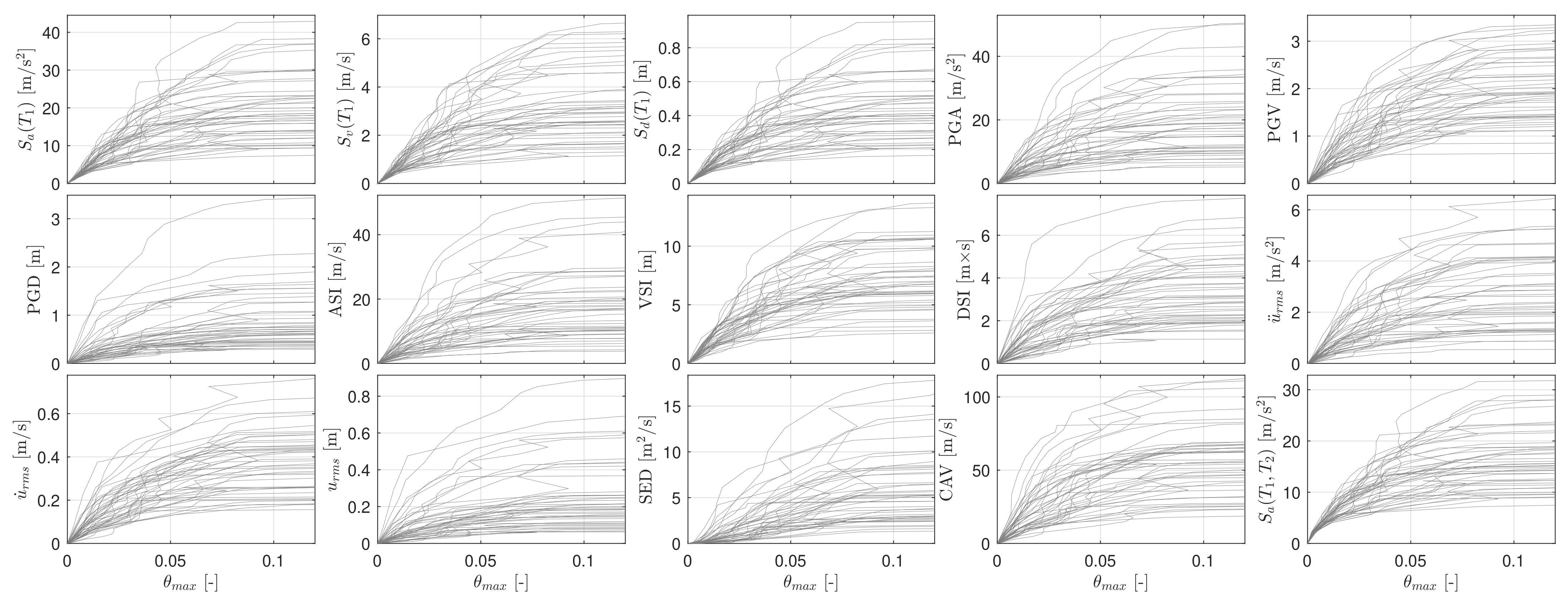
5.12. Direct IDA Based on Alternative IMs

Thus far, all the IDA and fragility functions have been presented only based on $S_a\left(T_1\right)$. While this is one of the optimal IM parameters in the majority of engineering structures, many researchers have found other single or compound IM parameters that are more efficient than $S_a\left(T_1\right)$ [62,63,64,65].

A series of alternative scalar time-dependent, frequency-dependent, and intensity-dependent IM parameters were collected by Hariri-Ardebili and Saouma [61]. While the mathematical expressions for these IMs are skipped in this paper, sixteen of them are studied and compared to the reference one, i.e., $S_a\left(T_1\right)$. We list them in the order they appear in this paper [66]:

• Spectral values at the fundamental period. IM${}_1$: $S_a\left(T_1\right)$, IM${}_2$: $S_v\left(T_1\right)$, IM${}_3$: $S_d\left(T_1\right)$.
• Peak value in the time domain. IM${}_4$: PGA, IM${}_5$: PGV, IM${}_6$: PGD.
• Spectral intensity values. IM${}_7$: ASI, IM${}_8$: VSI, IM${}_9$: DSI.
• Root mean square values. IM${}_{10}$: ${\ddot{u}}_{rms}$, IM${}_{11}$: ${\dot{u}}_{rms}$, IM${}_{12}$: $u_{rms}$.
• Others. IM${}_{13}$: SED, IM${}_{14}$: CAV.
• Higher-order spectral values. IM${}_{15}$: $S_a(T_1,T_2)$, IM${}_{16}$: $S_a(T_1,T_2,T_3)$

Figure 17 shows fifteen series of IDA curves (for only the RTR model of the four-story frame) based on different IM parameters. Qualitatively, various curves can be distinguished by their form and aggregation. A similar conclusion can be drawn for other frames and methods as well.

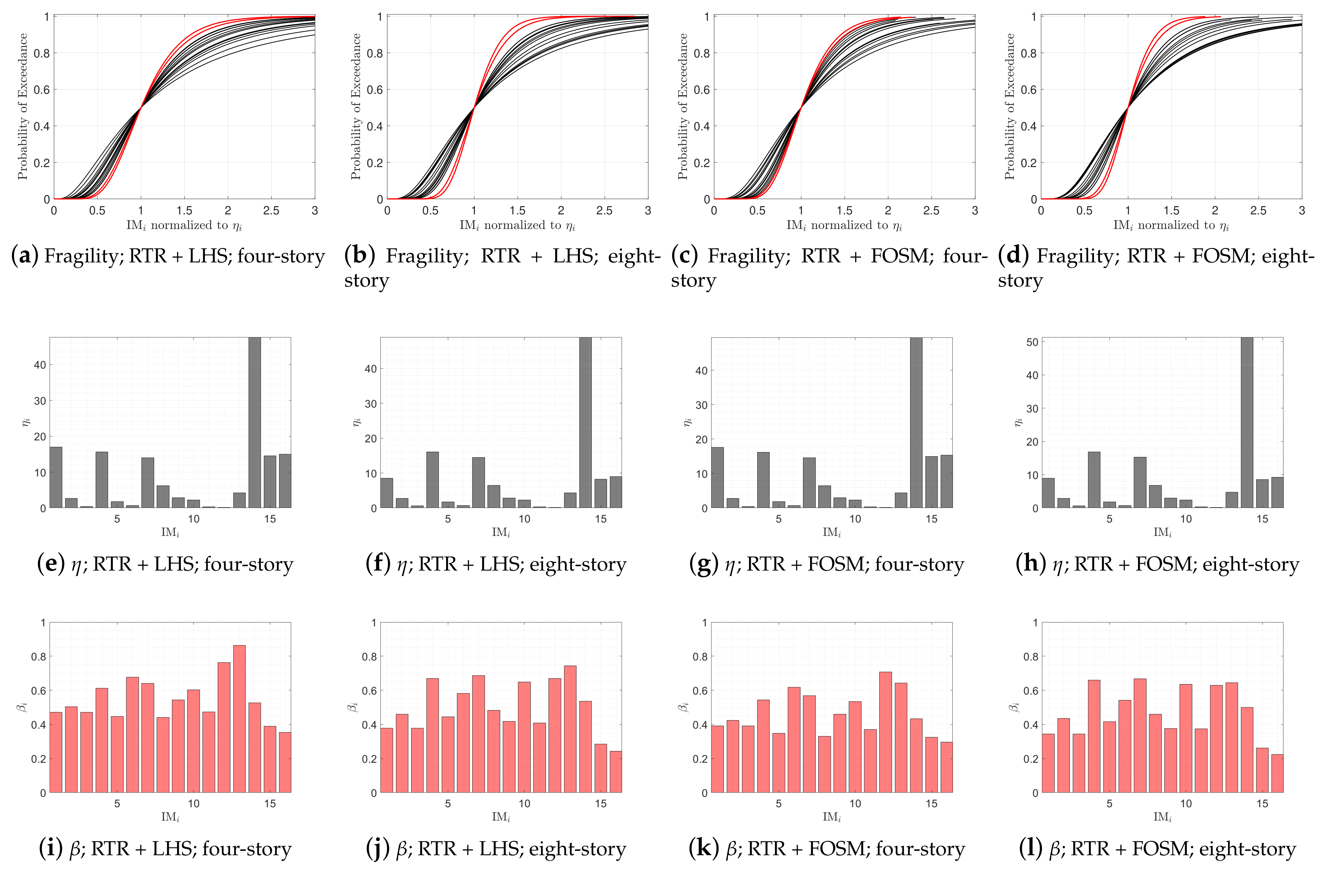
5.13. Sensitivity of Fragility Curves to Alternative IMs

While the previous section presented the IDA curves qualitatively, here, we quantify them in the form of collapse fragility curves. Consequently, sixteen fragility curves are derived for each IM parameter. Combining RTR with LHS/FOSM reliability methods yields $16\times 2=32$ curves, as seen in Figure 18a–d. As these sixteen curves have different natures (i.e., the x-axis in the fragility curve), the IM${}_i$ value of each curve is normalized by its ${\eta }_i$ value. Subsequently, all of them pass through one point $<\mathrm{IM}=1.0,\mathbb{P}=50\%>$. As can be seen, there is considerable variability among the normalized fragility curves. Among all the curves, the functions which are built on IM${}_{15}$ and IM${}_{16}$ (marked with red) are the most narrow ones. The median and logarithmic STD of these fragility functions are shown in Figure 18 (second and third columns). Overall, there is good consistency among $\eta$ and $\beta$ for different IM parameters from the two approaches; however, there are minor differences as well.

Compiling only the $\beta$ values, the following observations can be made:

• RTR + LHS (four-story): $S_a\left(T_1\right)$ = 0.47, $S_a(T_1,T_2)$ = 0.39, $S_a(T_1,T2,T3)$ = 0.35, SED = 0.86 (worst IM).
• RTR + LHS (eight-story): $S_a\left(T_1\right)$ = 0.38, $S_a(T_1,T_2)$ = 0.29, $S_a(T_1,T2,T3)$ = 0.24, SED = 0.74 (worst IM).
• RTR + FOSM (four-story): $S_a\left(T_1\right)$ = 0.39, $S_a(T_1,T_2)$ = 0.32, $S_a(T_1,T2,T3)$ = 0.29, $u_{rms}$ = 0.71 (worst IM).
• RTR + FOSM (eight-story): $S_a\left(T_1\right)$ = 0.34, $S_a(T_1,T_2)$ = 0.26, $S_a(T_1,T2,T3)$ = 0.22, PGA & ASI = 0.66 (worst IMs), (${\ddot{u}}_{rms}$, $u_{rms}$, and SED are very close to the worst IMs)
• $S_a(T_1,T2,T3)$ and $S_a(T_1,T_2)$ are the two most optimal IMs. This means that incorporating higher modes and their effective masses highly reduces the dispersion.
• SED is the worst IM for the four-story frame, while for the eight-story frame there is no unique worst IM parameter.

5.14. Impact of Within-Element and Between-Element Variability

Thus far, all the presented results have been founded on the assumption that all the RVs are fully correlated within the various elements of the frames. This means that a particular RV, such as RV1, has a fixed value when it is used for structural model i, RV1${}_i$, and its value only changes when the structural model is updated to j, RV1${}_j$. However, for various reasons (such as construction quality, aging, local damage, etc.) there might exist between-elements variability within one frame. This means that a particular RV1 takes different values of $\left\{{\mathrm{RV}}_i^1,{\mathrm{RV}}_i^2,\dots ,{\mathrm{RV}}_i^k\right\}$ when it is used to simulate model i, and a set of $\left\{{\mathrm{RV}}_j^1,{\mathrm{RV}}_j^2,\dots ,{\mathrm{RV}}_j^{k^{\prime }}\right\}$ when it is used to simulate model j (in general, k and $k^{\prime }$ might be identical or different). Depending on the degree of correlation, the model can be fully correlated (when all the elements in one model take the same value), partially correlated (when there are relations as to how the RV should vary from one element to the other), and uncorrelated (when arbitrary values are assigned for different elements within one model).

The within-element and between-element variability of modeling parameters is not a new topic, and has been studied in previously research. Kwon and Elnashai [24] reported that material spatial variability may change a structure’s failure mechanism. Vamvatsikos [67] compared the full and partial correlation cases for two design approaches (i.e., ductile and brittle) of a nine-story steel moment frame. In the ductile frame, the partial correlation assumption decreased the median IDA compared to full correlation. However, for the brittle frame, the findings were reversed. Gokkaya et al. [68] derived the standard deviation and correlation coefficients of modeling parameters based on multiple test groups. They compared the seismic responses of four different spatial correlation conditions and concluded that the uncorrelated case decreases the median and logarithmic standard deviation of IDA compared to the fully correlated case. Other studies have accentuated the significance of spatial correlation as well, among them [21,69,70].

This section compares the results of fully correlated and uncorrelated models. We assume that any partial correlation model will fall between these two upper and lower bounds. To generate the uncorrelated modeling parameters, separate datasets are generated and each is assigned to a different floor, thereby establishing floor-to-floor independence. These new models are hereafter called the “Uncorrelated Case”, while the previously analyzed models are called the “Correlated Case”. The comparison between these two groups is based on the RTR + LHS reliability analysis method.

Figure 19 compares the ${\theta }_{max}$-dependent median and dispersion and collapse fragility curves of the correlated and uncorrelated cases. The two methods of direct IDA and SPO2IDA are contrasted as well. Therefore, a total of four scenarios are compared. The results of the “only RTR” models are shown again for greater clarification. The following major observations can be made:

• The impact of variability on IDA and SPO2IDA medians begins at ${\theta }_{max}$ of 0.045 and 0.03, respectively, in the four-story frame. The corresponding ${\theta }_{max}$ values for the eight-story frame are 0.035 and 0.02, respectively.
• The uncorrelated assumption causes the IDA and SPO2IDA medians to decrease after the above-mentioned ${\theta }_{max}$ values are reached compared to the correlated models.
• The variability begins to affect the dispersion of IDA curves at ${\theta }_{max}$ values of 0.02 and 0.035 for the four-story and eight-story frames, respectively.
• The uncorrelated assumption causes the IDA dispersion to decrease after the above-mentioned ${\theta }_{max}$ values. However, the uncorrelation assumption does not significantly affect the SPO2IDA dispersion.
• In general, correlation does not have a significant efficacy on lower limit states; conversely, it decreases the median collapse capacity and dispersion values at higher limit states. These findings are aligned with the previously reported literature review.

6. Concluding Remarks

This paper aims to employ two reliability approaches including LHS and FOSM to evaluate the uncertainties inherent in the RTR variability and modeling parameters of beam-columns in two RC frames (four-story and eight-story) through two nonlinear analysis methods, namely, IDA and SPO2IDA. Considering (1) RTR only, (2) RTR + LHS, and (3) RTR + FOSM versus (A) IDA and (B) SPO2IDA, six combinations are analyzed for each frame, for a total of twelve groups. The results are compared in terms of dispersion values, fragility functions of various IM parameters, and fragility surfaces. In addition, several assumptions related to curve fitting, functional form, confidence intervals, and fragility uncertainties are investigated. The main outcomes are as follows:

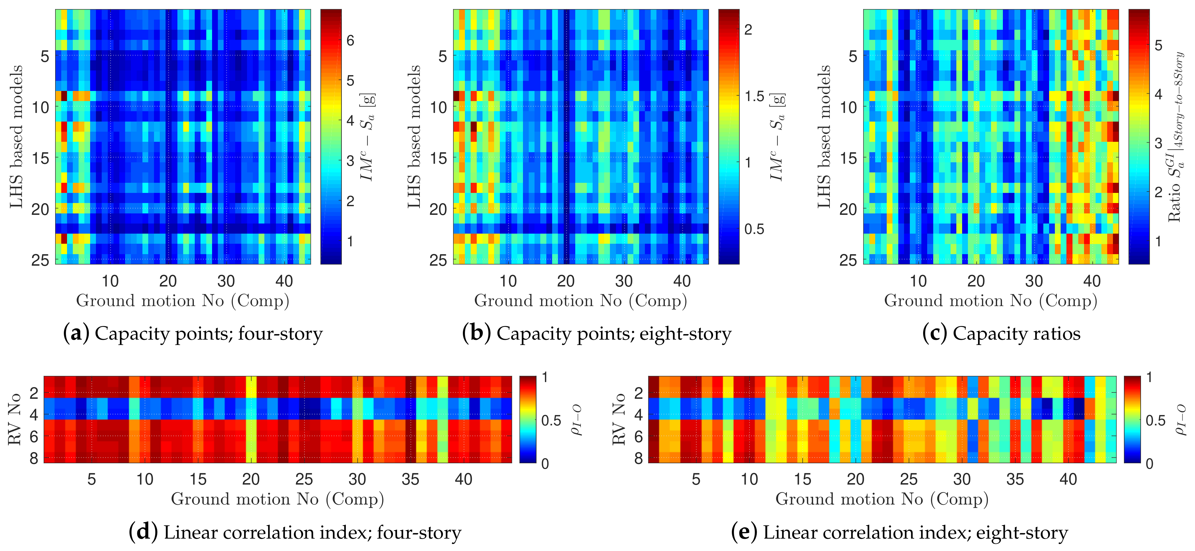
• The IM capacity point ratios fall in a wide range of 0.5 to 5.5 according to the LHS-based results for the two studied frames. This indicates that an impact of a “model-record” (structural model and ground motion record) combination is structure-dependent.
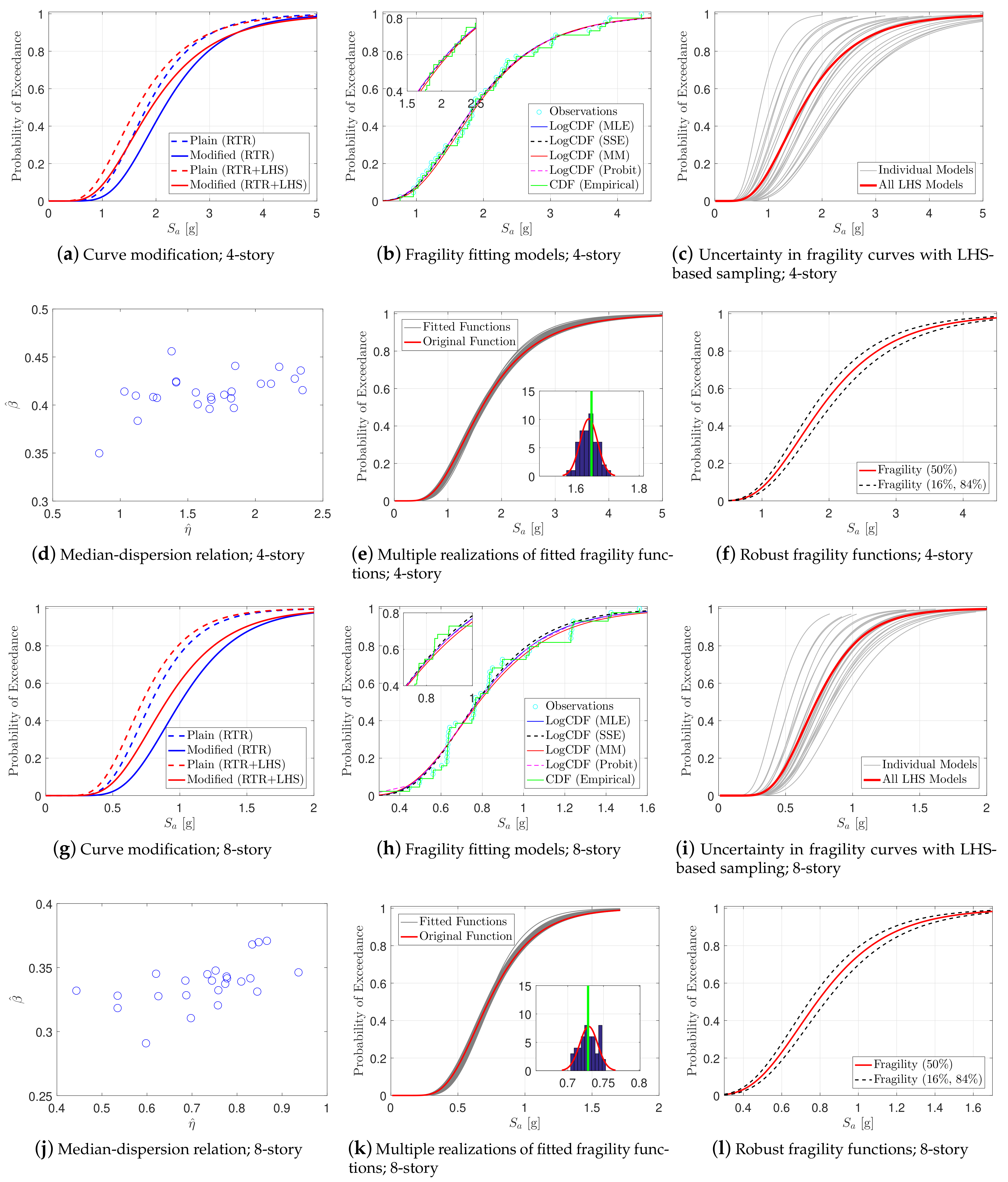
• The uncertainties associated with fragility curve fitting methods are negligible for the frames considered in this study.
• The uncertainties in the derivation of fragility functions can be quantified using the concept of robust fragility curves with a prescribed confidence interval while accounting for the joint probability distribution of the fragility model parameters.
• Both FOSM-based and LHS-based modeling uncertainties result in increasing the dispersion of the fragility curve as compared to RTR only.
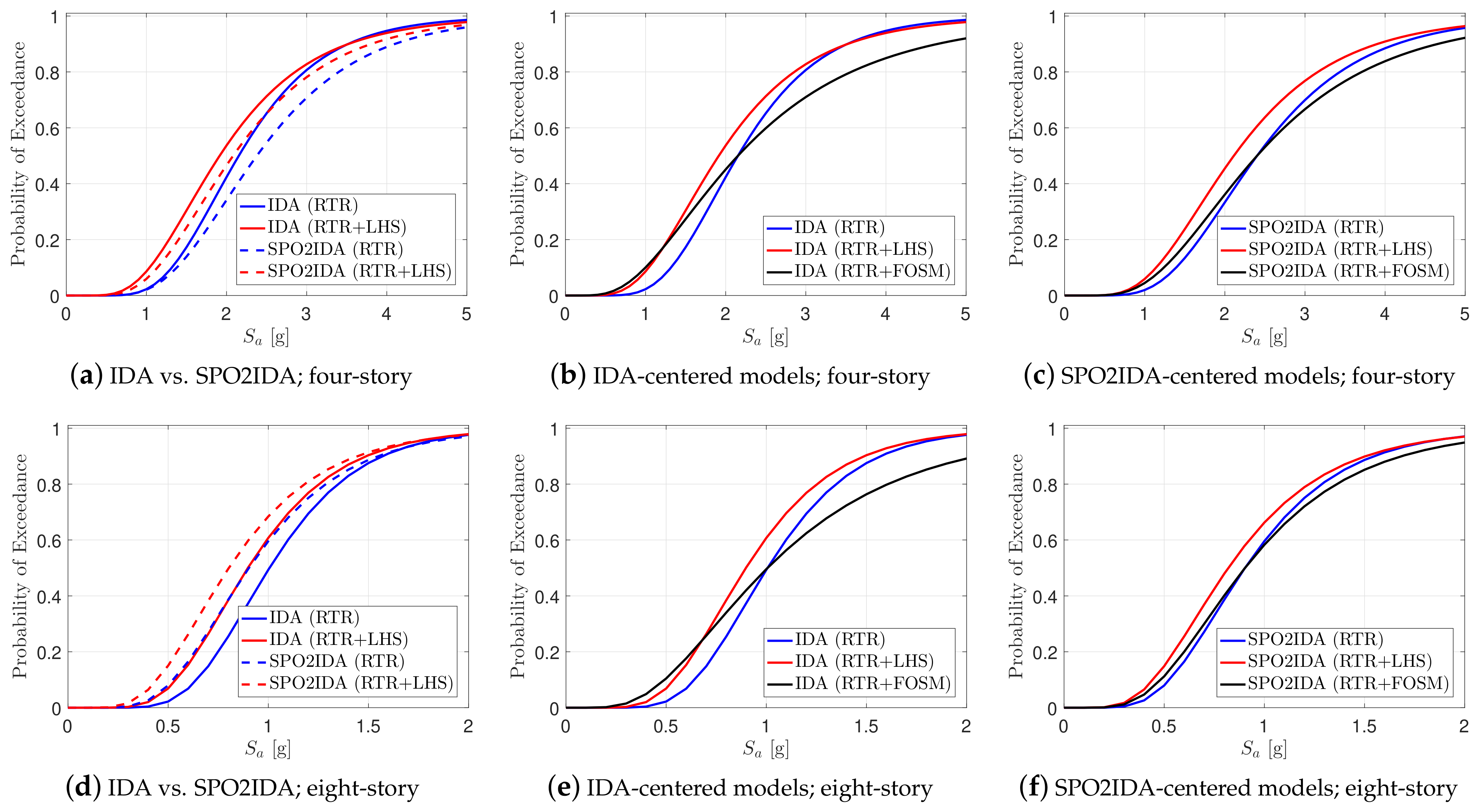
• In comparison with IDA, the SPO2IDA method overestimates the capacity curve of the four-story frame, while it underestimates the dispersion of the eight-story frame. At higher LSs, the dispersion of SPO2IDA is lower than that of IDA for the four-story frame, whereas the opposite trend is observed for the eight-story frame. In addition, the median fragility curve for SPO2IDA is higher than that of the direct IDA in the four-story frame, while the trend is vice versa in the case of the eight-story frame.
• The impact of modeling uncertainties in terms of median begins to diverge at 0.04 and 0.02 ${\theta }_{max}$ values for the four-story and eight-story frames, respectively. The dispersion varies between 0.35–0.65 at high LS for all combinations considered for both frames.
• The development of an “uncertain fragility region” to account for different combinations of reliability and analysis methods indicates that the uncertain fragility region becomes thicker and rotates more at higher seismic performance levels.
• The probability of exceedance of a particular combination of $<{\theta }_{max},S_a>$ for different analysis and reliability methods is presented in terms of fragility surfaces. The uncertainties in these fragility surfaces are then quantified by taking their mean and STD.
• Sixteen IM parameters are investigated by developing the corresponding IDA curves, which reveal various curves with distinct forms.
• The fragility curves derived based on sixteen IMs and for RTR with LHS/FOSM are diverse. Nonetheless, good consistency is observed between the two reliability approaches in terms of logarithmic STD and mean for different IM parameters.
• The IMs related to the higher-order spectral values yield the most optimal fragility curves among the various IMs considered in this paper. This indicates a remarkable decrease in dispersion when accounting for the higher modes and their effective masses.
• In general, the spatial correlation modeling assumption does not have a significant trace on lower limit states; conversely, the uncorrelated random variables assumption decreases the median collapse capacity and dispersion values at higher limit states.

References

- O’Hagan, A.; Oakley, J.E. Probability is perfect, but we can’t elicit it perfectly. Reliab. Eng. Syst. Saf. 2004, 85, 239–248. [Google Scholar] [CrossRef]
- Aslani, H.; Miranda, E. Probabilistic Earthquake Loss Estimation and Loss Disaggregation in Buildings. Ph.D. Thesis, Stanford University, Stanford, CA, USA, 2005. [Google Scholar]
- Ibarra, L.F.; Krawinkler, H. Global Collapse of Frame Structures under Seismic Excitations; Pacific Earthquake Engineering Research Center: Berkeley, CA, USA, 2005. [Google Scholar]
- Porter, K. An overview of PEER’s performance-based earthquake engineering methodology. In Proceedings of the 9th International Conference on Applications of Statistics and Probability in Civil Engineering (ICASP9), Francisco, CA, USA, 6–9 July 2003. [Google Scholar]
- Vamvatsikos, D.; Cornell, C. Incremental dynamic analysis. Earthq. Eng. Struct. Dyn. 2002, 31, 491–514. [Google Scholar] [CrossRef]
- Jalayer, F. Direct Probabilistic Seismic Analysis: Implementing Non-Linear Dynamic Assessments. Ph.D. Thesis, Stanford University, Stanford, CA, USA, 2003. [Google Scholar]
- Segura, C.; Sattar, S.; Hariri-Ardebili, M. Uncertainty in the Seismic Response of an RC Bridge Column due to Material Variability. ACI Struct. J. 2022, 119, 141–152. [Google Scholar]
- Ellingwood, B. Development of a Probability Based Load Criterion for American National Standard A58: Building Code Requirements for Minimum Design Loads in Buildings and Other Structures; US Department of Commerce, National Bureau of Standards: Gaithersburg, MD, USA, 1980; Volume 13.
- Ibarra, L.F.; Medina, R.A.; Krawinkler, H. Hysteretic models that incorporate strength and stiffness deterioration. Earthq. Eng. Struct. Dyn. 2005, 34, 1489–1511. [Google Scholar] [CrossRef]
- Panagiotakos, T.B.; Fardis, M.N. Deformations of reinforced concrete members at yielding and ultimate. Struct. J. 2001, 98, 135–148. [Google Scholar]
- Haselton, C.B.; Liel, A.B.; Taylor-Lange, S.C.; Deierlein, G.G. Calibration of Model to Simulate Response of Reinforced Concrete Beam-Columns to Collapse. ACI Struct. J. 2016, 113, 1141–1152. [Google Scholar] [CrossRef]
- Lignos, D.G.; Zareian, F.; Krawinkler, H. Reliability of a 4-story steel moment-resisting frame against collapse due to seismic excitations. In Proceedings of the Structures Congress 2008: Crossing Borders, Vancouver, BC, Canada, 24–26 April 2008; pp. 1–10. [Google Scholar]
- Haselton, C.; Deierlein, G. Assessing Seismic Collapse Safety of Modern Reinforced Concrete Moment Frame Buildings, Report No. TR 156; Technical Report; John A. Blume Earthquake Engineering Center Department of Civil Engineering: Stanford, CA, USA, 2006. [Google Scholar]
- Khojastehfar, E.; Beheshti-Aval, S.B.; Zolfaghari, M.R.; Nasrollahzade, K. Collapse fragility curve development using Monte Carlo simulation and artificial neural network. Proc. Inst. Mech. Eng. Part O J. Risk Reliab. 2014, 228, 301–312. [Google Scholar] [CrossRef]
- Asgarian, B.; Ordoubadi, B. Effects of structural uncertainties on seismic performance of steel moment resisting frames. J. Constr. Steel Res. 2016, 120, 132–142. [Google Scholar] [CrossRef]
- Ricci, P.; Manfredi, V.; Noto, F.; Terrenzi, M.; Petrone, C.; Celano, F.; De Risi, M.T.; Camata, G.; Franchin, P.; Magliulo, G.; et al. Modeling and seismic response analysis of Italian code-conforming reinforced concrete buildings. J. Earthq. Eng. 2018, 22, 105–139. [Google Scholar] [CrossRef]
- Badalassi, M.; Braconi, A.; Cajot, L.G.; Caprili, S.; Degee, H.; Gündel, M.; Hjiaj, M.; Hoffmeister, B.; Karamanos, S.A.; Salvatore, W.; et al. Influence of variability of material mechanical properties on seismic performance of steel and steel–concrete composite structures. Bull. Earthq. Eng. 2017, 15, 1559–1607. [Google Scholar] [CrossRef]
- British Standards Institution. Eurocode 8. Design of Structures for Earthquake Resistance. Assessment and Retrofitting of Buildings; British Standards Institution: London, UK, 2005. [Google Scholar]
- Barbato, M.; Zona, A.; Conte, J.P. Probabilistic nonlinear response analysis of steel-concrete composite beams. J. Struct. Eng. 2014, 140, 04013034. [Google Scholar] [CrossRef]
- Vamvatsikos, D.; Fragiadakis, M. Incremental dynamic analysis for estimating seismic performance sensitivity and uncertainty. Earthq. Eng. Struct. Dyn. 2010, 39, 141–163. [Google Scholar] [CrossRef]
- Kazantzi, A.; Vamvatsikos, D.; Lignos, D. Seismic performance of a steel moment-resisting frame subject to strength and ductility uncertainty. Eng. Struct. 2014, 78, 69–77. [Google Scholar] [CrossRef]
- Zareian, F.; Krawinkler, H.; Ibarra, L.; Lignos, D. Basic concepts and performance measures in prediction of collapse of buildings under earthquake ground motions. Struct. Des. Tall Spec. Build. 2010, 19, 167–181. [Google Scholar] [CrossRef]
- Dolšek, M. Incremental dynamic analysis with consideration of modeling uncertainties. Earthq. Eng. Struct. Dyn. 2009, 38, 805–825. [Google Scholar] [CrossRef]
- Kwon, O.S.; Elnashai, A. The effect of material and ground motion uncertainty on the seismic vulnerability curves of RC structure. Eng. Struct. 2006, 28, 289–303. [Google Scholar] [CrossRef]
- Kennedy, R.; Cornell, C.; Campbell, R.; Kaplan, S.; Perla, H. Probabilistic seismic safety study of an existing nuclear power plant. Nucl. Eng. Des. 1980, 59, 315–338. [Google Scholar] [CrossRef]
- Shinozuka, M.; Feng, M.; Lee, J.; Naganuma, T. Statistical analysis of fragility curves. J. Eng. Mech. 2000, 126, 1224–1231. [Google Scholar] [CrossRef]
- Baker, J. Efficient analytical fragility function fitting using dynamic structural analysis. Earthq. Spectra 2015, 31, 579–599. [Google Scholar] [CrossRef]
- Lallemant, D.; Kiremidjian, A.; Burton, H. Statistical procedures for developing earthquake damage fragility curves. Earthq. Eng. Struct. Dyn. 2015, 44, 1373–1389. [Google Scholar] [CrossRef]
- Miano, A.; Jalayer, F.; Ebrahimian, H.; Prota, A. Cloud to IDA: Efficient fragility assessment with limited scaling. Earthq. Eng. Struct. Dyn. 2018, 47, 1124–1147. [Google Scholar] [CrossRef]
- Mai, C.; Konakli, K.; Sudret, B. Seismic fragility curves for structures using non-parametric representations. Front. Struct. Civ. Eng. 2017, 11, 169–186. [Google Scholar] [CrossRef]
- Iervolino, I. Assessing uncertainty in estimation of seismic response for PBEE. Earthq. Eng. Struct. Dyn. 2017, 46, 1711–1723. [Google Scholar] [CrossRef]
- Baraschino, R.; Baltzopoulos, G.; Iervolino, I. R2R-EU: Software for fragility fitting and evaluation of estimation uncertainty in seismic risk analysis. Soil Dyn. Earthq. Eng. 2020, 132, 106093. [Google Scholar] [CrossRef]
- Baltzopoulos, G.; Baraschino, R.; Iervolino, I. On the number of records for structural risk estimation in PBEE. Earthq. Eng. Struct. Dyn. 2019, 48, 489–506. [Google Scholar] [CrossRef]
- De Risi, R.; Goda, K.; Tesfamariam, S. Multi-dimensional damage measure for seismic reliability analysis. Struct. Saf. 2019, 78, 1–11. [Google Scholar] [CrossRef]
- Basone, F.; Cavaleri, L.; Di Trapani, F.; Muscolino, G. Incremental dynamic based fragility assessment of reinforced concrete structures: Stationary vs. non-stationary artificial ground motions. Soil Dyn. Earthq. Eng. 2017, 103, 105–117. [Google Scholar] [CrossRef]
- Lemaire, M. Structural Reliability; John Wiley & Sons: Hoboken, NJ, USA, 2013. [Google Scholar]
- Ditlevsen, O.; Madsen, H.O. Structural Reliability Methods; Wiley: New York, NY, USA, 1996; Volume 178. [Google Scholar]
- Stein, M. Large sample properties of simulations using Latin hypercube sampling. Technometrics 1987, 29, 143–151. [Google Scholar] [CrossRef]
- Celarec, D.; Dolšek, M. The impact of modelling uncertainties on the seismic performance assessment of reinforced concrete frame buildings. Eng. Struct. 2013, 52, 340–354. [Google Scholar] [CrossRef]
- Cornell, C.A.; Jalayer, F.; Hamburger, R.O.; Foutch, D.A. Probabilistic basis for 2000 SAC federal emergency management agency steel moment frame guidelines. J. Struct. Eng. 2002, 128, 526–533. [Google Scholar] [CrossRef]
- Liel, A.; Haselton, C.; Deierlein, G.; Baker, J. Incorporating modeling uncertainties in the assessment of seismic collapse risk of buildings. Struct. Saf. 2009, 31, 197–211. [Google Scholar] [CrossRef]
- Matlab, R. Statistics Toolbox Release; The MathWorks Inc.: Natick, MA, USA, 2019. [Google Scholar]
- Der Kiureghian, A.; Liu, P.L. Structural reliability under incomplete probability information. J. Eng. Mech. 1986, 112, 85–104. [Google Scholar] [CrossRef]
- Liu, P.L.; Der Kiureghian, A. Multivariate distribution models with prescribed marginals and covariances. Probabilistic Eng. Mech. 1986, 1, 105–112. [Google Scholar] [CrossRef]
- Horn, R.; Johnson, C. Matrix Analysis; Cambridge University Press: Cambridge, UK, 1985. [Google Scholar]
- Vamvatsikos, D.; Allin Cornell, C. Direct estimation of the seismic demand and capacity of oscillators with multi-linear static pushovers through IDA. Earthq. Eng. Struct. Dyn. 2006, 35, 1097–1117. [Google Scholar] [CrossRef]
- Fragiadakis, M.; Vamvatsikos, D. Fast performance uncertainty estimation via pushover and approximate IDA. Earthq. Eng. Struct. Dyn. 2010, 39, 683–703. [Google Scholar] [CrossRef]
- FEMA P695. Quantification of Building Seismic Performance Factors; Technical Report Prepared by Applied Technology Council for the Federal Emergency Management Agency; FEMA: Washington, DC, USA, 2009.
- Franchin, P.; Ragni, L.; Rota, M.; Zona, A. Modelling uncertainties of Italian code-conforming structures for the purpose of seismic response analysis. J. Earthq. Eng. 2018, 22, 1964–1989. [Google Scholar] [CrossRef]
- Lignos, D. Sidesway Collapse of Deteriorating Structural Systems under Seismic Excitations; Stanford University: Stanford, CA, USA, 2008. [Google Scholar]
- Mazzoni, S.; McKenna, F.; Scott, M.H.; Fenves, G. The Open System for Earthquake Engineering Simulation (OpenSEES) User Command-Language Manual; Technical Report; Pacific Earthquake Engineering Research Center, University of California: Berkeley, CA, USA, 2006. [Google Scholar]
- McKenna, F. OpenSees: A framework for earthquake engineering simulation. Comput. Sci. Eng. 2011, 13, 58–66. [Google Scholar] [CrossRef]
- Poul, M.K.; Zerva, A. Time-domain PML formulation for modeling viscoelastic waves with Rayleigh-type damping in an unbounded domain: Theory and application in ABAQUS. Finite Elem. Anal. Des. 2018, 152, 1–16. [Google Scholar] [CrossRef]
- Haselton, C.; Baker, J.; Liel, A.; Deierlein, G. Accounting for ground-motion spectral shape characteristics in structural collapse assessment through an adjustment for epsilon. Struct. Eng. 2011, 137, 332–344. [Google Scholar] [CrossRef]
- Baker, J.; Cornell, C. A vector-valued ground motion intensity measure consisting of spectral acceleration and epsilon. Earthq. Eng. Struct. Dyn. 2005, 34, 1193–1217. [Google Scholar] [CrossRef]
- Zareian, F. Simplified Performance-Based Earthquake Engineering. Ph.D. Thesis, Stanford University, Stanford, CA, USA, 2006. [Google Scholar]
- Abrahamson, N.; Silva, W.J. Empirical response spectral attenuation relations for shallow crustal earthquakes. Seismol. Res. Lett. 1997, 68, 94–127. [Google Scholar] [CrossRef]
- Hariri-Ardebili, M.A.; Pourkamali-Anaraki, F. Structural uncertainty quantification with partial information. Expert Syst. Appl. 2022, 198, 116736. [Google Scholar] [CrossRef]
- Hariri-Ardebili, M.; Saouma, V. Collapse Fragility Curves for Concrete Dams: Comprehensive Study. ASCE J. Struct. Eng. 2016, 142, 04016075. [Google Scholar] [CrossRef]
- Jalayer, F.; De Risi, R.; Manfredi, G. Bayesian Cloud Analysis: Efficient structural fragility assessment using linear regression. Bull. Earthq. Eng. 2015, 13, 1183–1203. [Google Scholar] [CrossRef]
- Hariri-Ardebili, M.; Saouma, V. Probabilistic seismic demand model and optimal intensity measure for concrete dams. Struct. Saf. 2016, 59, 67–85. [Google Scholar] [CrossRef]
- Jankovic, S.; Stojadinovic, B. Probabilistic performance-based seismic demand model for {R/C} frame buildings. In Proceedings of the 13th World Conferance on Earthquake Engineering, Vancouver, BC, Canada, 1–6 August 2004. [Google Scholar]
- Mackie, K.; Stojadinovic, B. Comparison of Incremental Dynamic, Cloud, and Stripe methods for computing probabilistic seismic demand models. In Proceedings of the 2005 Structures Congress and the 2005 Forensic Engineering Symposium, New York, NY, USA, 20–24 April 2005. [Google Scholar]
- Tothong, P.; Luco, N. Probabilistic seismic demand analysis using advanced ground motion intensity measures. Earthq. Eng. Struct. Dyn. 2007, 36, 1837–1860. [Google Scholar] [CrossRef]
- Tondini, N.; Stojadinovic, B. Probabilistic seismic demand model for curved reinforced concrete bridges. Bull. Earthq. Eng. 2012, 10, 1455–1479. [Google Scholar] [CrossRef]
- Hariri-Ardebili, M.; Pourkamali-Anaraki, F. Matrix completion for cost reduction in finite element simulations under hybrid uncertainties. Appl. Math. Model. 2019, 69, 164–180. [Google Scholar] [CrossRef]
- Vamvatsikos, D. Seismic performance uncertainty estimation via IDA with progressive accelerogram-wise latin hypercube sampling. J. Struct. Eng. 2014, 140, A4014015. [Google Scholar] [CrossRef]
- Gokkaya, B.; Baker, J.; Deierlein, G. Estimation and impacts of model parameter correlation for seismic performance assessment of reinforced concrete structures. Struct. Saf. 2017, 69, 68–78. [Google Scholar] [CrossRef]
- Idota, H.; Guan, L.; Yamazaki, K. Statistical correlation of steel members for system reliability analysis. In Proceedings of the 9th international conference on structural safety and reliability (ICOSSAR), Osaka, Japan, 13–17 September 2009. [Google Scholar]
- Liu, Z.; Atamturktur, S.; Juang, C.H. Reliability based multi-objective robust design optimization of steel moment resisting frame considering spatial variability of connection parameters. Eng. Struct. 2014, 76, 393–403. [Google Scholar] [CrossRef]