Strategic Environmental Assessment of Land Transportation: An Application of DEA with Undesirable Output Approach

Abstract

The efficiency of land transportation contributes significantly to determining a country’s economic and environmental sustainability. The examination of land transportation efficiency encompasses performance and environmental efficiency to improve system performance and citizen satisfaction. Evaluating the efficiency of land transportation is a vital process to improve operation efficiency, decrease investment costs, save energy, reduce greenhouse gas emissions, and enhance environmental protection. There are many methods for measuring transportation efficiency, but few papers have used the input and output data to evaluate the ecological efficiency of land transportation. This research focuses on evaluating the environmental efficiency for land transportation by using the data envelopment analysis (DEA) method with undesirable output to handle unwanted data. By using this, the paper aims to measure the performance of land transportation in 25 Organization for Economic Co-operation and Development (OECD) countries in the period of 2015–2019, considered as 25 decision-making units (DMUs) in the model. For identifying the ranking of DMUs, four inputs (infrastructure investment and maintenance, length of transport routes, labor force, and energy consumption) are considered. At the same time, the outputs consist of freight transport and passenger transport as desirable outputs and carbon dioxide emission (CO₂) as an undesirable output. The proposed model effectively determines the environment-efficient DMUs in a very time-efficient manner. Managerial implications of the study provide further insight into the investigated measures and offer recommendations for improving the environmental efficiency of land transportation in OECD countries.

1. Introduction

As the economy becomes more developed, the demand for goods circulation between areas, countries, or regions in the world increases rapidly. Especially in the current era of globalization, transportation plays a vital role in linking local and global economies, shortening the geographical distance to reduce costs, reducing commodity prices, and promoting trade development. According to the International Transport Forum (ITF) forecast, the demand for global transportation will rapidly increase during the next three decades; the total transport activity is expected to more than double by 2050 under the trajectory reflecting the current trend. Inside, passenger transport demand will grow 2.3 times, and freight transport demand will increase 2.6 times [1].

Land transport consists of three modes: road, rail, and pipeline; inland waterways (IWW) transport is also added in some European studies. However, because pipeline transport has a completely different specificity, this type of transport is often omitted in topics related to land transport. Land transportation involves road and rail transportation modes that play a central role in passenger and freight transportation, with a fast-growing market share. Land transport significantly facilitates economic growth; physical capital accumulation is another driving force, mainly in developed countries [2]. The road is the most popular transport due to flexibility, compatibility, speed, and low cost [3]. In 2013, road freight transport accounted for approximately 72% of total inland freight in the European Union, while inland waterways, rail, and pipelines collectively accounted for the remaining 28% [4]. Rail transport carries the competitive advantage of less energy usage and environmental improvement [5], with about 54 tons CO₂ emission that arises to ship 12 tons goods from China to inland Europe by airway, compared to 3.3 tons by maritime and railway, and 2.8 tons by railway across the Landbridge [6].

Transportation is one of the critical elements that burn fossil fuels (oil, coal, etc.), releasing vast amounts of carbon dioxide (CO₂) and other toxic gases into the atmosphere, creating the greenhouse effect. Shankar et al. [7] indicate that the transportation sector is responsible for 23% of global CO₂ emissions. Land transportation contributes to climate change and is the primary source of CO₂ emissions and one of the most challenging sectors to decarbonize in many countries [8]. The specific number varies by country, but it is virtually always a significant contributor to this effect. In the 2015 Paris Agreement, 195 world countries negotiated to combat climate change, focusing on reducing greenhouse gas emissions and preventing global warming from worsening [9]. Governments have set their own Intended Nationally Defined Contribution (INDC) objectives based on their respective national circumstances to archive the global greenhouse gas emissions reduction. Germany is committed to a target to reduce 40% of the greenhouse gas emissions levels by 2030 compared to 1990. USA national target for 2025 is to reduce greenhouse gas emissions by 26–28% compared to 2005. Japan expected to make more effort to decrease by 26% their greenhouse gas emissions in 2030 compared to 2013 levels while contributing to the global climate change solution [10]. Since 2000, European Transport Ministers have shared the requirement for consistent decision-making processes on transport systems towards sustainability [11]. Despite the efforts of many countries to cut CO₂ emissions, current trends indicate that atmospheric carbon dioxide will increase for most countries by the end of the year 2040 [12,13]. It requires in-depth research and analysis on land passenger and freight transport and specifying the role of land transportation in the overall emissions problem.

Land transportation involves congestion, energy consumption, air and noise pollution, deterioration of infrastructure, safety problems that contribute to non-sustainable effects on the environment, economy, and society sectors [14]. The efficiency of land transportation can contribute considerably to assessing the sustainable development of the economy and environment of countries. Land transportation efficiency evaluation includes performance and environmental efficiency to improve system performance and citizen satisfaction. Over the last decade, researchers and practitioners have become extremely conscious of transportation performance on sustainability. Controversial interests of different stakeholders frequently conflict within a single pillar of sustainability (i.e., social conflicts; economic conflicts; conflicts over environmental issues; preferences), and, therefore, balancing their interests regarding one pillar is sometimes more in the foreground than to balance social, economic, and environmental aspects [15,16]. Evaluating the efficiency of land transportation can improve operation efficiency, decrease investment costs, save energy, reduce greenhouse gas emissions, and enhance environmental protection. There are many methods for measuring transportation efficiency, but few papers have used the input and output data to evaluate the environmental efficiency of land transportation.

Based on the previous discussion, the hypothesis was formulated, evaluating the efficiency of land transportation is a vital process to improve operation efficiency, decrease investment costs, save energy, reduce greenhouse gas emissions, and enhance environmental protection. This research focuses on estimating the environmental efficiency for land transportation by using a DEA undesirable output model that overcomes previous models to handle unwanted data. The purpose of the present study is to propose the DEA undesirable output model for measuring the performance of land transportation of 25 OECD countries as 25 decision-making units (DMUs). Differences in infrastructure investment, the demand for transport, and the length of routes are the factors that identify the ranking of DMUs. The research process is visualized in Figure 1. The model is used as an explicit function of four inputs (infrastructure investment and maintenance, length of transport routes, labor force, and energy consumption). The outputs consist of freight transport and passenger transport as desirable outputs, while carbon dioxide emission (CO₂) is considered as an undesirable output. The outcome of this study can support the government or policymakers in evaluating and improving the environmental efficiency of land transportation or many more related industries.

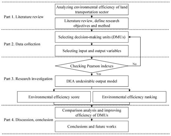
Figure 1. The structure of the research process.

The structure of this paper is organized as follows: Section 2 is the literature review. Section 3 explains the method approach. The case study is included in Section 4. The obtained results are presented in Section 5. Finally, the discussions, conclusions, and future studies are summarized in Section 6 and Section 7.

2. Literature Review

Data envelopment analysis (DEA) is one of the most popular tools for evaluating the efficiency of decision-making units (DMUs) based on different inputs and outputs. DEA analysis was introduced in 1978 from the initiative by Charnes, Cooper, and Rhodes (CCR) [17]. However, ideas on efficiency evaluation appeared many years early. Farrell proposed production possibility frontier (PPF) as a criterion for measuring (relative) efficiency among enterprises in the same industry using two components including allocation efficiency and overall technical efficiency in 1957 [18]. The CCR method used the non-parameter methodology to create a PPF curve regard on collected data of DMUs [17]. Then the efficiency scores for those DMUs were calculated and compared using a variety of mathematical programming models. Banker, Charnes, and Cooper (BCC) improved the CCR model to the BCC model by including variable returns to scale (VRS) situations in the calculation in 1984 [19]. The resulting BCC model provided a more specific analysis of the efficiency of DMUs.

There are a plethora of studies that focused on multi-aspects of transport to evaluate efficiency as operation, investment, infrastructure, energy, and environment. For instance, Yu and Lin [20] proposed the multi-activity network DEA model considering both production and consumption technologies to measure efficiency in railway performance. To compare the CO₂-sensitive productivity development of the European commercial transport industry, Krautzberger and Wetzel [21] employed the Malmquist–Luenberger productivity index to investigate country-specific regulations’ effects on productivity and identify innovative countries. Zhou et al. [22] conducted a study of carbon dioxide emissions performance of China’s transport sector using the undesirable out-put-oriented DEA models with a different return of scales. Chu et al. [23] utilized the SBM-DEA model with parallel computing design for environmental efficiency evaluation in the big data context with a transportation system application. Jiang et al. [24] applied DEA to the transportation system efficiency evaluation, aiming at redundant construction, unreasonable utilization of resources, and other issues. Wu et al. [25] introduced a DEA common-weight evaluation framework for resource reallocation and target setting to enhance the environmental performance of regional highway transportation systems in China. Stefaniec et al. [26] proposed a triple bottom line-based network DEA approach for the assessment of inland transportation in China, considering social, economic, and environmental dimensions of sustainability. Musolino et al. [27] evaluated the efficiency in transportation planning by comparison between DEA and multi-criteria decision-making.

To assess the economic and environmental efficiency of global airlines, Chang et al. [28] introduced an extended environmental slacks-based measure data envelopment analysis model (SBM-DEA undesirable output) with the weak disposability assumption. A new model, the virtual frontier benevolent DEA cross efficiency model (VFB-DEA) model, is proposed in a study by Cui and Li [29] to evaluate energy efficiency for airlines. Zhang et al. [30] used the SBM-DEA model with undesirable outputs to measure and compare the energy efficiency and productivity of Chinese and American airlines. Shirazi and Mohammadi [31] evaluated the efficiency of Iranian airlines by developing a robust slack-based measure (SBM) model that was developed by adding undesirable outputs and uncertainty to consider the practical situations. Applications of DEA approaches in various studies regarding inputs, outputs, DMUs, and applied areas are summarized in Table A1.

This research is devoted to bridging the gap of the existing literature of transportation systems efficiency by simultaneously considering economic and environmental sustainability, with the determination of factors influencing the land transportation systems in the OECD context through literature and experts’ responses. For this evaluation, the DEA method is an effective and practical method to determine the most efficient DMUs among a group of DMUs. The model is used as an explicit function of four inputs (infrastructure investment and maintenance, length of transport routes, labor force, and energy consumption). The outputs consist of freight transport and passenger transport as desirable outputs, while carbon dioxide emission (CO₂) is considered undesirable outputs. The outcome of this study can assist governments and policymakers in evaluating and improving the environmental efficiency of land transportation or related industry.

3. Methodology

3.1. Data Envelopment Analysis (DEA)

Data envelopment analysis (DEA), i.e., linear programming, is a non-parametric approach for measuring the relative efficiency of decision-making units (DMUs) by comparing multiple inputs with outputs in the framework of frontier analysis in terms of attempting to decrease inputs or increase outputs [32,33]. The DEA model’s objective is to maximize the ratio of weighted outputs to weighted inputs for the considered DMUs, which is described in the model (1).

$$\begin{gathered} Max Z_{pq}=Max\frac{{\displaystyle \sum }outputs}{{\displaystyle \sum }inputs}=\frac{{{\displaystyle \sum }}_{i=1}^s{u}_{ip}{y}_{iq}}{{{\displaystyle \sum }}_{j=1}^t{v}_{jp}{x}_{jq}} \\ \mathrm{such} \mathrm{that} \\ 0\le \frac{{{\displaystyle \sum }}_{i=1}^s{u}_{ip}{y}_{iq}}{{{\displaystyle \sum }}_{j=1}^t{v}_{jp}{x}_{jq}}\le 1, q=1, 2,\dots ,n \\ q=1, 2,\dots ,n \\ {u}_{ip}\ge \in i=1,2,\dots ,s \\ {v}_{jp}\ge \in j=1,2,\dots ,t \end{gathered}$$

(1)

where $Z_{pq}$ is the relative efficiency of DMUq $\left(q=1,2,\dots ,n\right)$ when evaluated using the weights associated with DMUp $\left(p=1,2,\dots ,n\right)$; $n$ is number of evaluated DMUs; $s$ is number of outputs; $t$ number of inputs; $u_{ip}$ is the weight attached to $i^{th}$ output $\left(i=1,2,\dots ,s\right)$ for DMUp $\left(p=1,2,\dots ,n\right)$; $v_{jp}$ is the weight attached to $j^{th}$ input $\left(j=1,2,\dots ,t\right)$ for DMUp $\left(p=1,2,\dots ,n\right)$; $y_{iq}$ is value of $i^{th}$ output $\left(i=1,2,\dots ,s\right)$ for DMUq $\left(q=1,2,\dots ,n\right)$; $x_{jq}$ is value of $j^{th}$ input $\left(j=1,2,\dots ,t\right)$ for DMUq $\left(q=1,2,\dots ,n\right)$; $\in$ is infinitesimal constant.

We assume that there are 25 DMUs that represent 25 OECD countries (the value of $q$ ranges from 1 to 25, $\left(q=1,2,\dots ,q=25\right)$). This paper considers four inputs including infrastructure investment and maintenance, length of transport routes, labor force, and energy consumption (the value of $j$ ranges from 1 to 4, $\left(j=1,2,\dots ,t=4\right)$), while freight transport, passenger transport, CO₂ emission are considered as outputs (the value of $i$ ranges from 1 to 3, $\left(i=1,2,\dots ,s=3\right)$).

From model (1), the considered DMUs satisfy the necessary condition as DEA efficiency if the efficiency score, i.e., the optimal value of the objective function is at 1 (or 100%). Otherwise, they are considered as DEA inefficiency.

DEA is a non-parametric method, which is a powerful research technique because this method does not require the assumption of normality for data. In the DEA model, homogeneity and isotonicity are two essential models’ assumptions. Before applying the DEA model, the correlation between inputs and outputs must be verified, which means that it should be in a total positive linear correlation (when the value of one variable increases, the other variable value will also increase). The correlation coefficient formula of Pearson’s ($r$) of two variables ($x$) and ($y$) is measured as Equation (2) [34].

$$r_{xy}=\frac{{{\displaystyle \sum }}_{i=1}^n\left(x_i-\overline{x}\right)\left(y_i-\overline{y}\right) }{\sqrt{{{\displaystyle \sum }}_{i=1}^n{\left(x_i-\overline{x}\right)}^2{{\displaystyle \sum }}_{i=1}^n{\left(y_i-\overline{y}\right)}^2}}$$

(2)

where n is the size of the sample; $x_i,y_i$ denotes the individual sample points indexed with $i$; $\overline{x}=\frac{1}{\mathrm{n}}{\displaystyle \sum }_{i=1}^n{x}_i$ is the mean of the sample which is analogous for $\overline{y}$.

3.2. DEA Undesirable Output Model

The aim of this study is to develop a framework to measure the environmental efficiency and potential CO₂ reduction of the transportation sector in 25 OECD countries by incorporating the undesirable output into the objective function. The model assumes that reducing input resources (infrastructure investment and maintenance, length of transport routes, labor force, and energy consumption) and undesirable output (bad output and CO₂ emission) relative to producing more desirable outputs (freight transport and passenger transport) is a criterion for efficiency measurement.

DEA undesirable output model tackles the bad outputs during efficiency and inefficiency analysis. When considering an undesirable output in the model, it should be noted that efficiency can be formed with more desirable output relative to less undesirable output and less input resources.

The outputs of this study of evaluating the environmental efficiency of land transportation appear to be undesirable (CO₂ emission). Halkos and Petrou [35] presented a critical review of the methods for dealing with undesirable outputs in DEA models. This research applied the undesirable output model (BadOutput-C), which is implemented by DEA Solver software. The methodology process is presented as follows [36,37].

The matrices of inputs and outputs of the DMUs will be standing for $\left(x_{0 },y_0\right)$. The outputs of the matrix $y$ will be disintegrated into undesirable outputs ($Y^b$) and desirable outputs are $Y^g$. Each country will be declared as DMU $\left(x_0, y_0^g, y_0^b\right)$.

The production possibility set is presented in Equation (3).

$$P=\left\{ \left(x, y^g, y^b\right) {\displaystyle |}\begin{array}{c} x \ge X\lambda , y^g\le Y^g\lambda , y^b\ge Y^b\lambda \\ L \le e\lambda \le U, \lambda \ge 0\end{array}\right\}$$

(3)

where $\lambda$ is the intensity vector; $L$ is the lower bound; $U$ is the upper bound of $\lambda$.

In the existence of bad output, a DMU $\left(x_0, y_0^g, y_0^b\right)$ is efficient if there is no vector $\left(x, y^g, y^b\right) \in P$ such that $x_{0 }\ge x, y_0^g\le y^g,y_{0 }^b\ge y^b$ having at least one inequality.

The adjustment of SBM to obtain the undesirable output model is calculated, as can be seen in Equation (4).

$${\rho }^{*}=\min \frac{1-\frac{1}{m} {{\displaystyle \sum }}_{i=1}^m\frac{s_{io}^{-}}{x_{io}}}{1+\frac{1}{s} \left({{\displaystyle \sum }}_{r=1}^{s_1}\frac{s_r^g}{y_{ro}^g}+{{\displaystyle \sum }}_{r=1}^{s_2}\frac{s_r^b}{y_{ro}^b} \right)}$$

(4)

constraint to $x_0=X\lambda +s^{-}; y_0^g=Y\lambda -s^g; y_0^b=Y\lambda +s^b;L\le e\lambda \le U; s^{-}, s^g, s^b, \lambda \ge 0.$

The excesses in inputs, bad outputs, lack of good outputs are expressed by the vector $s^{-}$, $s^b$, and $s^g$, respectively. $s_1$ and $s_2$ are the number of components in $s^b,$ $s^g,$ and s = $s_1+s_2.$

A DMU $\left(x_0, y_0^g, y_0^b\right)$ is efficient if ${\rho }^{*}=1$. Otherwise, ${\rho }^{*}<1$, i.e., $s^{-*}=s^{b*}=s^{g*}$.

Through Charnes–Cooper transformation approach, the fractional model can be transformed into the linear model with the consequential variables $v, u^g, \mathrm{and} u^b$ for the constant return to scale, i.e., $L=0,U=\infty$, as in Equations (5)–(9).

$$\mathrm{Max}{u}^g{y}_o^g-v{x}_o-u^b{y}_o^b$$

(5)

such that

$$u^g{Y}^g-vX-u^b{y}^b\le 0$$

(6)

$$v\ge \frac{1}{m}{\left[\raisebox{1ex}{$1$}\!\left/ \!\raisebox{-1ex}{$x_o$}\right.\right]}^{ }$$

(7)

$$u^g\ge \frac{1+u^g{y}_o^g-v{x}_o-u^b{y}_o^b}{s} {\left[\raisebox{1ex}{$1$}\!\left/ \!\raisebox{-1ex}{$y_o^g$}\right.\right]}^{ }$$

(8)

$$u^b\ge \frac{1+u^g{y}_o^g-v{x}_o-u^b{y}_o^b}{s} {\left[\raisebox{1ex}{$1$}\!\left/ \!\raisebox{-1ex}{$y_o^b$}\right.\right]}^{ }$$

(9)

where $v$, $u^b$, and $u^g$ are assigned as the virtual costs of inputs, bad outputs, and good outputs, respectively.

The weights of good and bad outputs must be set in accordance with $w_1,w_2$, respectively. Then, the model computed the relative weights as $W_1=s{w}_1/\left(w_1+w_2\right)$ and $W_2=s{w}_2/\left(w_1+w_2\right)$. The objective function will be converted to Equation (10). In this research, the authors used the default value with $w_1=w_2=1$.

$${\rho }^{*}=\min \frac{1-\frac{1}{m} {{\displaystyle \sum }}_{i=1}^m\frac{s_{io}^{-}}{x_{io}}}{1+\frac{1}{s} \left(W_1{{\displaystyle \sum }}_{r=1}^{s_1}\frac{s_r^g}{y_{ro}^g}+W_2{{\displaystyle \sum }}_{r=1}^{s_2}\frac{s_r^b}{y_{ro}^b} \right)}$$

(10)

4. A Case Study in OECD Countries

4.1. Selection of Decision-Making Units (DMUs)

This section analyses the data used to measure the performance of the land transportation system of 25 OECD countries as the DMUs that are shown in Table 1. The data availability of this study covers the period from 2015 to 2019.

Table 1. List of OECD countries and their GDP (unit: billion USD).

No.	Countries	Symbol	GDP in 2019	No.	Countries	Symbol	GDP in 2019
1	Australia	AUS	1396.57	14	Italy	ITA	2004.91
2	Austria	AUT	445.08	15	Japan	JPN	5064.87
3	Belgium	BEL	533.25	16	Korea	KOR	1646.74
4	Switzerland	CHE	731.47	17	Lithuania	LTU	54.64
5	Czech Republic	CZE	250.69	18	Latvia	LVA	34.06
6	Germany	DEU	3861.12	19	The Netherlands	NLD	907.05
7	Denmark	DNK	350.10	20	Norway	NOR	405.51
8	Spain	ESP	1393.49	21	Poland	POL	595.86
9	Finland	FIN	268.97	22	Slovak Republic	SVK	105.12
10	France	FRA	2715.52	23	Sweden	SWE	531.28
11	United Kingdom	GBR	2830.81	24	Turkey	TUR	761.43
12	Greece	GRC	205.33	25	United States	USA	21,433.22
13	Hungary	HUN	163.50

4.2. Selection of Input and Output Variables

The evaluation criteria were chosen through a review of existing literature. Various input and output variables from previous research were enumerated in Table A1. For analyzing transportation efficiency, researchers have used several different inputs and outputs, such as operational costs, capital investment, the number of passengers, freight volume, the number of vehicles, labor, fuel, passenger, and freight turnover volume, revenue, CO₂ emission, and GHG.

Based on the literature review on the previous studies and the data availability, this study selects four input variables, including infrastructure investment and maintenance, length of transport routes, labor force, and energy consumption. Three variables are selected for output indicators, including freight transport, passenger transport, and CO₂ emission. It is important to note that CO₂ emission is considered an undesirable output factor in this study.

The DEA structure of the operating process for land transportation efficiency evaluation and the inputs, and outputs selection are visualized in Figure 2. The description of input and output variables is presented as follows

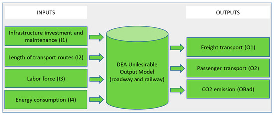
Figure 2. The DEA structure of the operating process for land transportation efficiency evaluation.

• Infrastructure investment and maintenance (input, unit in million USD): includes spending on new construction, preservation, and improvement of the existing transportation network. This indicator is measured in million USD for the road, rail, and inland by year.
• Length of transport routes (input, unit in km): the total length of transport routes available for the use of roadway and railway vehicles.
• Labor force (input, unit in thousands of persons): consists of all the people who are of the right age to work, in a country or area.
• Energy consumption (input, unit in thousand tons of oil equivalent): covers the total energy consumed by transport modes: roadway (buses, truck, etc.), railway (trains, metro, etc.), waterway, airway, and pipeline transport.
• Freight transport (desirable output, unit in million ton-kilometers): refers to the physical process of shipping commodities, goods, and cargo by using inland transportation mode on the national network.
• Passenger transport (desirable output, unit in million passenger-kilometers): is the process of transport for passengers by using inland transportation mode on the national network.
• CO₂ emission (undesirable output, unit in million tons): exclusively refers to gross direct emissions stemming from the combustion of fuels.

For the selection of evaluation criteria, there are some limitations of the research such as the inability to obtain data separately for passenger and freight transport. Another weakness is that only road and rail transport are investigated as part of land transport. Furthermore, the inability to decompose energy consumption and CO₂ emission by other modes for all analyzed OECD economies is a drawback of the study, but land transport constitutes the vast majority in all analyzed entities. In future research, however, researchers are recommended to pay more attention to these aspects. Regarding employment, transport is the bloodstream of the economy which participates directly or indirectly in all economic processes. It also influences the professional activity of people. The global production of modern economies is the result not only of technology, capital, energy, but also of the workforce. Since transport participates in meeting the needs of society and economy, it is reasonable to include the entire workforce in the study.

4.3. Data Sources

The data used in this research comprised information for 25 DMUs from 2015 to 2019. The infrastructure investment and maintenance, passenger and freight transport, and CO₂ emission from the fuel are collected in the databases of the OECD official website [38]. The total length routes were obtained from OECD [38] and UNECE Transport Statistics Database [39]. The labor force is found in The World Bank Group report [40]. The final energy consumption for the transport sector is from the European statistics website [41].

The descriptive statistics on input and output variables of the land transportation including roadway and railway for the period from 2015 to 2019 including maximum value, minimum value, average value, and standard deviation, are presented in Table 2. Transportation infrastructures have a difference in investment among countries. In 2015, the infrastructure investment and maintenance in the USA is the highest with 157,327 million USD, while the lowest is in Latvia with 812 million USD, and 242.28 million USD 18,062 on average. The USA also has the largest energy consumption with 718,375 KTOE in 2019, which is 650 times higher than that of the minimum.

Table 2. Statistics on input and output variables of land transportation.

Statistics	Input Variables				Output Variables
	I1	I2	I3	I4	O1	O2	OBad
Year Period of 2015
Max	157,327	6,837,065	160,656,132	686,389	5,437,097	6,429,086	4929
Min	812	48,085	1,008,427	1038	14,927	2823	7
Average	18,062	568,596	21,080,306	45,243	347,801	571,310	416
SD	31,619	1,321,773	32,595,195	131,924	1,048,669	1,249,388	959
Year Period of 2016
Max	162,536	6,813,074	162,618,460	700,186	5,323,380	6,547,948	4838
Min	577	48,097	1,006,975	1034	15,518	2771	7
Average	18,329	569,395	21,300,773	46,269	347,191	582,208	413
SD	32,944	1,317,344	32,980,854	134,553	1,026,567	1,272,221	941
Year Period of 2017
Max	162,580	6,816,884	164,326,552	705,947	5,400,580	6,591,557	4761
Min	615	48,122	1,003,671	1081	18,145	2742	7
Average	18,694	569,911	21,493,977	46,784	355,351	588,451	411
SD	32,863	1,318,064	33,315,752	135,633	1,041,429	1,280,353	926
Year Period of 2018
Max	166,142	6,860,371	165,551,383	717,309	5,494,692	6,697,201	4910
Min	639	48,126	1,000,161	1109	17,659	2809	7
Average	19,059	572,394	21,685,309	47,287	362,101	595,374	413
SD	33,403	1,326,309	33,600,628	137,814	1,059,600	1,299,751	953
Year Period of 2019
Max	1,718,319	7,003,524	167,329,067	718,375	5,235,465	6,790,757	4744
Min	5899	48,128	983,777	1102	16,010	2785	7
Average	189,574	580,484	21,845,299	47,397	354,203	604,001	398
SD	343,154	1,353,572	33,943,033	138,017	1,009,555	1,317,480	921

5. Results Analysis

5.1. Pearson Correlation

A requirement before employing DEA is input and output variables have isotonic relationships. This means that increasing any input should not bring a decrease to any output. Therefore, Pearson’s correlation analysis is employed to check this prerequisite. The correlation coefficient between inputs and outputs is shown in Table 3. It shows the correlation coefficients between four input variables and three output variables are all more than 0.503, indicating inputs and outputs have a significantly positive relationship.

Table 3. Correlation matrix of input and output variables (2015–2019).

	I1	I2	I3	I4	O1	O2	OBad
Infrastructure investment and maintenance (I1)	1	0.542	0.551	0.529	0.503	0.554	0.531
Length of transport routes (I2)	0.542	1	0.938	0.983	0.981	0.984	0.982
Labor force (I3)	0.551	0.938	1	0.919	0.903	0.968	0.967
Energy consumption (I4)	0.529	0.983	0.919	1	0.994	0.982	0.982
Freight transport (O1)	0.503	0.981	0.903	0.994	1	0.968	0.975
Passenger transport (O2)	0.554	0.984	0.968	0.982	0.968	1	0.989
CO2 emission (OBad)	0.531	0.982	0.967	0.982	0.975	0.989	1

Note: all Pearson correlations are significant at the 0.01 level (2-tailed).

5.2. Environmental Efficiency and Ranking

The overall efficiency of the land transportation systems in 25 OECD countries for the whole period based on the DEA model with undesirable outputs is calculated using DEA software.

Table 4 presents the efficiency score of the land transport and ranking for each country from 2015 to 2019. For efficiency of land transportation Australia, Switzerland, Spain, France, Italy, Japan, Korea, Lithuania, The Netherlands, Poland, Sweden, and the USA ranks first among all 25 countries in five consecutive years with the efficiency score is at 1 for the whole periods. The efficiency score of Greece is less than 0.5 that is the worst country in 2015–2018. The worst efficiency country in 2019 is Latvia (efficiency score of 0.3074). Germany has the highest efficiency (efficiency score of 1) in the two years 2015 and 2016, and the performance decreased in the three after year.

Table 4. Efficiency evaluation results of the land transportation sector.

Countries	2015		2016		2017		2018		2019
	Score	Rank	Score	Rank	Score	Rank	Score	Rank	Score	Rank
Australia	1.0000	1	1.0000	1	1.0000	1	1.0000	1	1.0000	1
Austria	0.5123	23	0.4840	23	0.4171	23	0.4526	24	0.4210	24
Belgium	0.6974	18	0.6432	19	0.6162	17	0.5727	19	0.5324	18
Switzerland	1.0000	1	1.0000	1	1.0000	1	1.0000	1	1.0000	1
Czech Republic	0.6216	21	0.5721	21	0.4887	21	0.4839	22	0.4432	23
Germany	1.0000	1	1.0000	1	0.8379	14	0.8165	14	0.7239	13
Denmark	0.5925	22	0.5476	22	0.5062	20	0.4942	21	0.4461	22
Spain	1.0000	1	1.0000	1	1.0000	1	1.0000	1	1.0000	1
Finland	0.7241	17	0.6132	20	0.6217	16	0.6206	17	0.5989	16
France	1.0000	1	1.0000	1	1.0000	1	1.0000	1	1.0000	1
United Kingdom	0.6552	19	0.6511	18	0.5971	18	0.6152	18	0.5790	17
Greece	0.3037	25	0.3158	25	0.2511	25	0.2945	25	0.4464	21
Hungary	0.6221	20	0.6652	17	0.5235	19	0.5146	20	0.4679	19
Italy	1.0000	1	1.0000	1	1.0000	1	1.0000	1	1.0000	1
Japan	1.0000	1	1.0000	1	1.0000	1	1.0000	1	1.0000	1
Korea	1.0000	1	1.0000	1	1.0000	1	1.0000	1	1.0000	1
Lithuania	1.0000	1	1.0000	1	1.0000	1	1.0000	1	1.0000	1
Latvia	1.0000	1	1.0000	1	0.3309	24	1.0000	1	0.3074	25
The Netherlands	1.0000	1	1.0000	1	1.0000	1	1.0000	1	1.0000	1
Norway	0.5020	24	0.4823	24	0.4506	22	0.4592	23	0.4465	20
Poland	1.0000	1	1.0000	1	1.0000	1	1.0000	1	1.0000	1
Slovak Republic	1.0000	1	1.0000	1	1.0000	1	0.7772	15	0.6372	14
Sweden	1.0000	1	1.0000	1	1.0000	1	1.0000	1	1.0000	1
Turkey	0.7636	16	0.6733	16	0.6695	15	0.6365	16	0.6199	15
United States	1.0000	1	1.0000	1	1.0000	1	1.0000	1	1.0000	1

The trend of efficiency score of the land transportation for each year from 2015 to 2019 by countries is visualized in Figure 3. The results show that a general decreasing trend of efficiency of the land transportation system. It can be seen clearly in most countries such as Belgium, Czech Republic, United Kingdom, Germany, Denmark, and Turkey. From 2016 to 2019, the efficiency score of Austria, Greece, and Norway is less than 0.5.

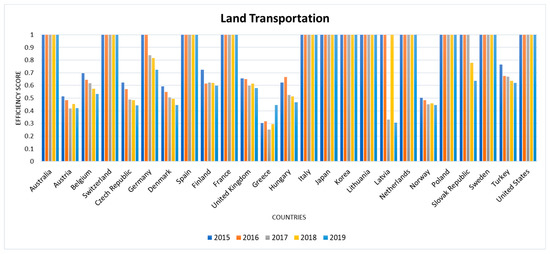
Figure 3. Efficiency score of the land transportation.

Figure 4 illustrates the average efficiency of land transportation from the view of space-time. The average efficiency declined by 9%, from 0.8398 in 2015 to 0.7468 in 2019. For the nations with low efficiency (Austria, Denmark, Greece, and Norway), the raw data demonstrates that the total length of transport routes is smaller than the average total length of transport routes of 25 OECD countries. The raw data also indicates that the average passenger transport and freight transport of 25 OECD countries are higher than passenger transport and freight transport in Austria, Denmark, Greece, and Norway.

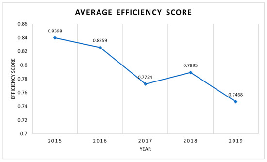
Figure 4. Average efficiency score of the land transportation.

6. Discussions

Figure 5 and Figure 6 show the relationship between the average efficiency and environmental variables including energy consumption and CO₂ emissions. We can observe that most countries such as Australia, Japan, Korea, and the USA consume a large amount of energy, but the efficiency is also higher than other countries. On the other hand, Greece, Austria, and Norway are three countries that accounted for the lowest efficiency score despite their consumption of a small amount of energy. The nations that have high CO₂ emissions are high operation efficiency.

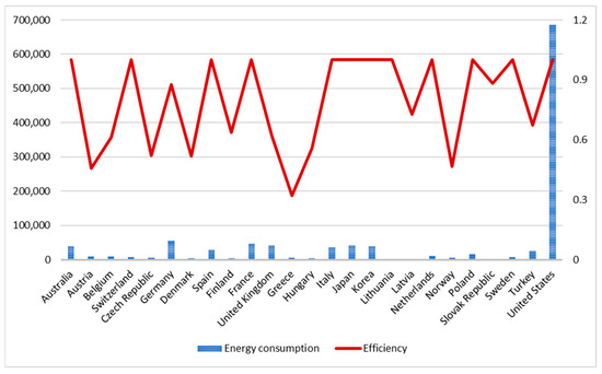
Figure 5. Comparison between average efficiency and energy consumption.

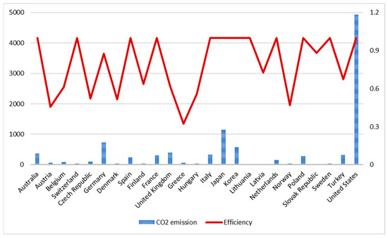
Figure 6. Comparison between average efficiency and CO₂ emissions.

When the efficiency score equals 1, the DMUs are considered efficient; otherwise, it is ineffective. The efficiency of DMUs can be improved based on the projections of inefficient. Table A2 presents the projections of input and output variables for improving efficiency, as an example for the period of 2019. As a result, Greece which has the lowest efficiency score and higher rank should decrease the variables including the length of transport routes, labor, energy consumption, and CO₂ emission by more than 53% to obtain the efficient frontier. Austria should reduce all the input variables and CO₂ emissions by more than 49% to achieve an efficiency score of 1. For DMU Latvia, a plan to achieve efficiency of 1, a reduction in infrastructure investment and maintenance of 39%, in the length of transport routes of 41%, in the labor force of 35%, in the energy consumption of 16%, and increase in freight transport of 415% would be required. Czech Republic, Germany, United Kingdom, Finland, and Hungary can be improved efficiency by reducing of all input variables including infrastructure investment and maintenance, length of transport routes, labor force, and energy consumption; as well as the CO₂ emission decrease following the percentage in Table A2. The other countries may reduce or increase different input and out variables in order to obtain efficiency. It is conspicuous that nations can improve the environmental efficiency of the land transportation networks. However, it is difficult to apply in practice, such as passenger and freight transport depending on the demand of customers. Besides, due to sustainable development considerations, the reduction of the undesirable output variable (CO₂ emission) must be a priority.

7. Conclusions

The DEA method is thought to be an excellent approach to evaluate the relative efficiency of DMUs with many inputs and outputs, and it does not require determining the relationships between inputs and outputs through subjective assumptions. In this research, we used DEA with an undesirable output model to measure the environmental efficiency of land transportation in 25 OECD countries for the period 2015–2019. It uses infrastructure investment and maintenance, the length of transport routes, labor, and energy consumption as inputs. The model’s outputs are total passenger and freight transport and CO₂ emission. As a result, the list of countries with the best efficiency score for land transportation includes Australia, Switzerland, Spain, France, Italy, Japan, Korea, Lithuania, The Netherlands, Poland, Sweden, and the USA. The average overall efficiency of land transportation systems in 25 OECD countries expresses decreasing trend. For managerial implications, this study could be a significant material for stakeholders, i.e., governments, and authorities in evaluating and improving the environmental efficiency of land transportation or many more related industries. The DEA-based approach assists in implying those countries who have not been utilizing their resources to generate the best possible outcomes in land transportation (those with low efficiency). Therefore, there is huge space for them to improve their efficiency performance, in which the improvement can be achieved by more efficient use of their current resources, rather than increasing the resources. The reason behind the change can be traced to political and/or economic situations.

The current study has the following limitations which also signify the avenues for future research. First, it will be of both academic and practical values to find the root cause of the intertemporal efficiency change of the countries. The decomposition method used in this paper sheds a light on the problem, but the root cause should be traced to deeper reasons, such as economic structures, political, and cultural factors. Third, DEA itself cannot provide statistical inference on the significance of the city assessment results. A remedy for this problem is to augment DEA with bootstrapping [42]. For future studies, other input and output factors that affect the environmental efficiency of the land transportation sector should be considered, for example, vehicle in use, GDP, road accidents, NOx emissions, and SOx emissions. This paper only considers roadway and railway that represent land transportation sector. Future studies should investigate other transport modes such as pipeline, inland waterway, or air transport. In terms of methodologies approach, future studies should combine DEA with multi-criteria decision-making (MCDM) models, such as (fuzzy) WASPAS, VIKOR, EDAS, and ELECTRE, to name a few, [43] and analyze the results with sensitivity of criteria, or comparative analysis of methods [44], to enhance the results’ robustness.

References

- ITF. ITF Transport Outlook Project. Available online: https://www.itf-oecd.org/ (accessed on 9 December 2021).
- Park, J.S.; Seo, Y.J.; Ha, M.H. The Role of Maritime, Land, and Air Transportation in Economic Growth: Panel Evidence from OECD and Non-OECD Countries. Res. Transp. Econ. 2019, 78, 100765. [Google Scholar] [CrossRef]
- Reis, V.; Meier, J.F.; Pace, G.; Palacin, R. Rail and Multi-Modal Transport. Res. Transp. Econ. 2013, 41, 17–30. [Google Scholar] [CrossRef]
- Behrends, S. Burden or Opportunity for Modal Shift?—Embracing the Urban Dimension of Intermodal Road-Rail Transport. Transp. Policy 2017, 59, 10–16. [Google Scholar] [CrossRef]
- McKinnon, A.C. Logistics and the Environment. In Handbook of Transport and the Environment (Volume 4); Hensher, D.A., Button, K.J., Eds.; Emerald Group Publishing Limited: Bingley, UK, 2003; pp. 665–685. [Google Scholar]
- Pomfret, R. The Eurasian Landbridge: Implications of Linking East Asia and Europe by Rail. Res. Glob. 2021, 3, 100046. [Google Scholar] [CrossRef]
- Shankar, R.; Pathak, D.K.; Choudhary, D. Decarbonizing Freight Transportation: An Integrated EFA-TISM Approach to Model Enablers of Dedicated Freight Corridors. Technol. Forecast. Soc. Change 2019, 143, 85–100. [Google Scholar] [CrossRef]
- Giannakis, E.; Serghides, D.; Dimitriou, S.; Zittis, G. Land Transport CO2 Emissions and Climate Change: Evidence from Cyprus. Int. J. Sustain. Energy 2020, 39, 634–647. [Google Scholar] [CrossRef]
- The Paris Agreement. Available online: https://unfccc.int/process-and-meetings/the-paris-agreement/the-paris-agreement (accessed on 9 December 2021).
- Dong, C.; Dong, X.; Jiang, Q.; Dong, K.; Liu, G. What Is the Probability of Achieving the Carbon Dioxide Emission Targets of the Paris Agreement? Evidence from the Top Ten Emitters. Sci. Total Environ. 2018, 622–623, 1294–1303. [Google Scholar] [CrossRef]
- Russo, F.; Rindone, C. Regional Transport Plans: From Direction Role Denied to Common Rules Identified. Sustainability 2021, 13, 9052. [Google Scholar] [CrossRef]
- Mohmmed, A.; Li, Z.; Arowolo, A.O.; Su, H.; Deng, X.; Najmuddin, O.; Zhang, Y. Driving Factors of CO2 Emissions and Nexus with Economic Growth, Development and Human Health in the Top Ten Emitting Countries. Resour. Conserv. Recycl. 2019, 148, 157–169. [Google Scholar] [CrossRef]
- Jiang, J.; Ye, B.; Liu, J. Research on the Peak of CO2 Emissions in the Developing World: Current Progress and Future Prospect. Appl. Energy 2019, 235, 186–203. [Google Scholar] [CrossRef]
- Russo, F.; Pellicanò, D.S. Planning and Sustainable Development of Urban Logistics: From International Goals to Regional Realization. WIT Trans. Ecol. Environ. 2019, 238, 59–72. [Google Scholar]
- Kyburz-Graber, R.; Hofer, K.; Wolfensberger, B. Studies on a Socio-ecological Approach to Environmental Education: A Contribution to a Critical Position in the Education for Sustainable Development Discourse. Environ. Educ. Res. 2006, 12, 101–114. [Google Scholar] [CrossRef] [Green Version]
- Mieg, H.A. Sustainability and Innovation in Urban Development: Concept and Case. Sustain. Dev. 2012, 20, 251–263. [Google Scholar] [CrossRef]
- Charnes, A.; Cooper, W.W.; Rhodes, E. Measuring the Efficiency of Decision Making Units. Eur. J. Oper. Res. 1978, 2, 429–444. [Google Scholar] [CrossRef]
- Farrell, M.J. The Measurement of Productive Efficiency. J. R. Stat. Soc. Ser. A (Gen.) 1957, 120, 253–281. [Google Scholar] [CrossRef]
- Banker, R.D.; Charnes, A.; Cooper, W.W. Some Models for Estimating Technical and Scale Inefficiencies in Data Envelopment Analysis. Manag. Sci. 1984, 30, 1078–1092. [Google Scholar] [CrossRef] [Green Version]
- Yu, M.M.; Lin, E.T.J. Efficiency and Effectiveness in Railway Performance Using a Multi-Activity Network DEA Model. Omega 2008, 36, 1005–1017. [Google Scholar] [CrossRef]
- Krautzberger, L.; Wetzel, H. Transport and CO2: Productivity Growth and Carbon Dioxide Emissions in the European Commercial Transport Industry. Environ. Resour. Econ. 2012, 53, 435–454. [Google Scholar] [CrossRef] [Green Version]
- Zhou, G.; Chung, W.; Zhang, X. A Study of Carbon Dioxide Emissions Performance of China’s Transport Sector. Energy 2013, 50, 302–314. [Google Scholar] [CrossRef]
- Chu, J.-F.; Wu, J.; Song, M.-L. An SBM-DEA Model with Parallel Computing Design for Environmental Efficiency Evaluation in the Big Data Context: A Transportation System Application. Ann. Oper. Res. 2018, 270, 105–124. [Google Scholar] [CrossRef]
- Jiang, G.-J.; Liu, L.; Lv, H.-D. Transportation System Evaluation Model Based on DEA. J. Discret. Math. Sci. Cryptogr. 2017, 20, 115–124. [Google Scholar] [CrossRef]
- Wu, J.; Chu, J.; An, Q.; Sun, J.; Yin, P. Resource Reallocation and Target Setting for Improving Environmental Performance of DMUs: An Application to Regional Highway Transportation Systems in China. Transp. Res. Part D Transp. Environ. 2018, 61, 204–216. [Google Scholar] [CrossRef]
- Stefaniec, A.; Hosseini, K.; Xie, J.; Li, Y. Sustainability Assessment of Inland Transportation in China: A Triple Bottom Line-Based Network DEA Approach. Transp. Res. Part D Transp. Environ. 2020, 80, 102258. [Google Scholar] [CrossRef]
- Musolino, G.; Rindone, C.; Vitetta, A. Evaluation in Transport Planning: A Comparision between Data Envelopment Analysis and Multi Criteria Decision Making Methods. In Proceedings of the 31st Annual European Simulation and Modelling Conference, ESM 2017, Lisbon, Portugal, 25–27 October 2017; pp. 233–237. [Google Scholar]
- Chang, Y.T.; Park, H.-S.; Jeong, J.-B.; Lee, J.-W. Evaluating Economic and Environmental Efficiency of Global Airlines: A SBM-DEA Approach. Transp. Res. Part D Transp. Environ. 2014, 27, 46–50. [Google Scholar] [CrossRef]
- Cui, Q.; Li, Y. Evaluating Energy Efficiency for Airlines: An Application of VFB-DEA. J. Air Transp. Manag. 2015, 44–45, 34–41. [Google Scholar] [CrossRef]
- Zhang, J.; Fang, H.; Wang, H.; Jia, M.; Wu, J.; Fang, S. Energy Efficiency of Airlines and Its Influencing Factors: A Comparison between China and the United States. Resour. Conserv. Recycl. 2017, 125, 1–8. [Google Scholar] [CrossRef]
- Shirazi, F.; Mohammadi, E. Evaluating Efficiency of Airlines: A New Robust DEA Approach with Undesirable Output. Res. Transp. Bus. Manag. 2019, 33, 100467. [Google Scholar] [CrossRef]
- Azadeh, A.; Ghaderi, S.F.; Nasrollahi, M.R. Location Optimization of Wind Plants in Iran by an Integrated Hierarchical Data Envelopment Analysis. Renew. Energy 2011, 36, 1621–1631. [Google Scholar] [CrossRef]
- Wang, C.-N.; Dang, T.-T.; Nguyen, N.-A.-T. Location Optimization of Wind Plants Using DEA and Fuzzy Multi-Criteria Decision Making: A Case Study in Vietnam. IEEE Access 2021, 9, 116265–116285. [Google Scholar] [CrossRef]
- Wang, C.-N.; Dang, T.-T.; Nguyen, N.-A.-T.; Le, T.-T.-H. Supporting Better Decision-Making: A Combined Grey Model and Data Envelopment Analysis for Efficiency Evaluation in E-Commerce Marketplaces. Sustainability 2020, 12, 10385. [Google Scholar] [CrossRef]
- Halkos, G.; Petrou, K.N. Treating Undesirable Outputs in DEA: A Critical Review. Econ. Anal. Policy 2019, 62, 97–104. [Google Scholar] [CrossRef]
- Cecchini, L.; Venanzi, S.; Pierri, A.; Chiorri, M. Environmental Efficiency Analysis and Estimation of CO2 Abatement Costs in Dairy Cattle Farms in Umbria (Italy): A SBM-DEA Model with Undesirable Output. J. Clean. Prod. 2018, 197, 895–907. [Google Scholar] [CrossRef]
- Puri, J.; Yadav, S.P. A Fuzzy DEA Model with Undesirable Fuzzy Outputs and Its Application to the Banking Sector in India. Expert Syst. Appl. 2014, 41, 6419–6432. [Google Scholar] [CrossRef]
- OECD Annual Statistics. Available online: https://www.oecd-ilibrary.org/transport/data/itf-transport-statistics/annual-transport-statistics_4785726e-en?fbclid=IwAR06Bf1FwnScZjbHeAnAAkpg7v0bRu5sh4p_sQMY84eoBKKsnntA88X-e58 (accessed on 9 December 2021).
- UNECE Transport Statistics Database. Available online: https://w3.unece.org/PXWeb/en/TableDomains/?fbclid=IwAR3FEbhpxmi3d7C7vXL_vUk_pnQQdnFEZyt5RdyA6AaoCb57O_iNUXdX0a8 (accessed on 9 December 2021).
- Worldbank Database. Available online: https://databank.worldbank.org/home.aspx?fbclid=IwAR2_NtPiUvij8g3GN6PEXXn2IK7vzf4bstCNNCd_23AGCJZPlFcWGEqCWD4 (accessed on 9 December 2021).
- European Statistics. Available online: https://ec.europa.eu/eurostat/web/main/data/database?fbclid=IwAR13lcTcQACPV9hytY3Dx7j2yIfQN-XA1qmWfe-MDUfOAkB4STRIBOVIKtw (accessed on 9 December 2021).
- Simar, L.; Wilson, P.W. Sensitivity Analysis of Efficiency Scores: How to Bootstrap in Nonparametric Frontier Models. Manag. Sci. 1998, 44, 49–61. [Google Scholar] [CrossRef] [Green Version]
- Nguyen, N.B.T.; Lin, G.-H.; Dang, T.-T. A Two Phase Integrated Fuzzy Decision-Making Framework for Green Supplier Selection in the Coffee Bean Supply Chain. Mathematics 2021, 9, 1923. [Google Scholar] [CrossRef]
- Wang, C.-N.; Nguyen, N.-A.-T.; Dang, T.-T.; Hsu, H.-P. Evaluating Sustainable Last-Mile Delivery (LMD) in B2C E-Commerce Using Two-Stage Fuzzy MCDM Approach: A Case Study from Vietnam. IEEE Access 2021, 9, 146050–146067. [Google Scholar] [CrossRef]
Publisher’s Note: MDPI stays neutral with regard to jurisdictional claims in published maps and institutional affiliations. |
© 2022 by the authors. Licensee MDPI, Basel, Switzerland. This article is an open access article distributed under the terms and conditions of the Creative Commons Attribution (CC BY) license (https://creativecommons.org/licenses/by/4.0/).