
Modeling a Practical Dual-Fuel Gas Turbine Power Generation System Using Dynamic Neural Network and Deep Learning


Abstract
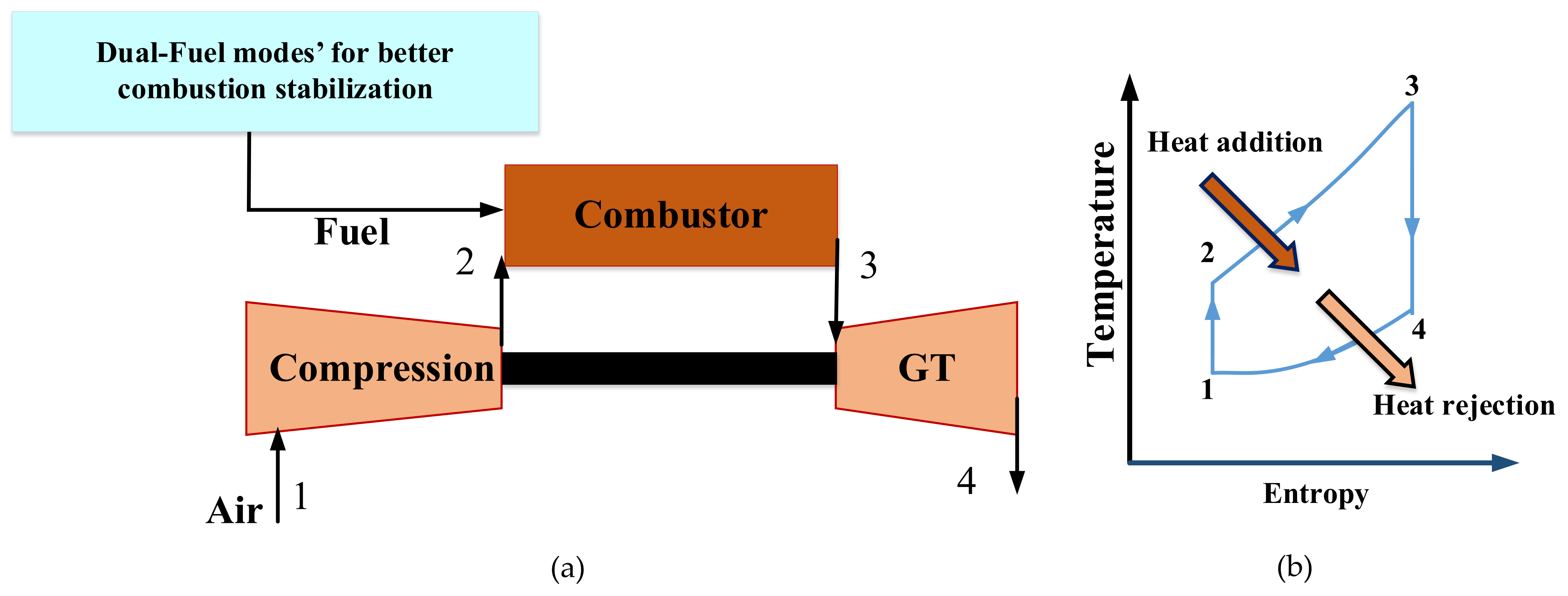
:1. Introduction
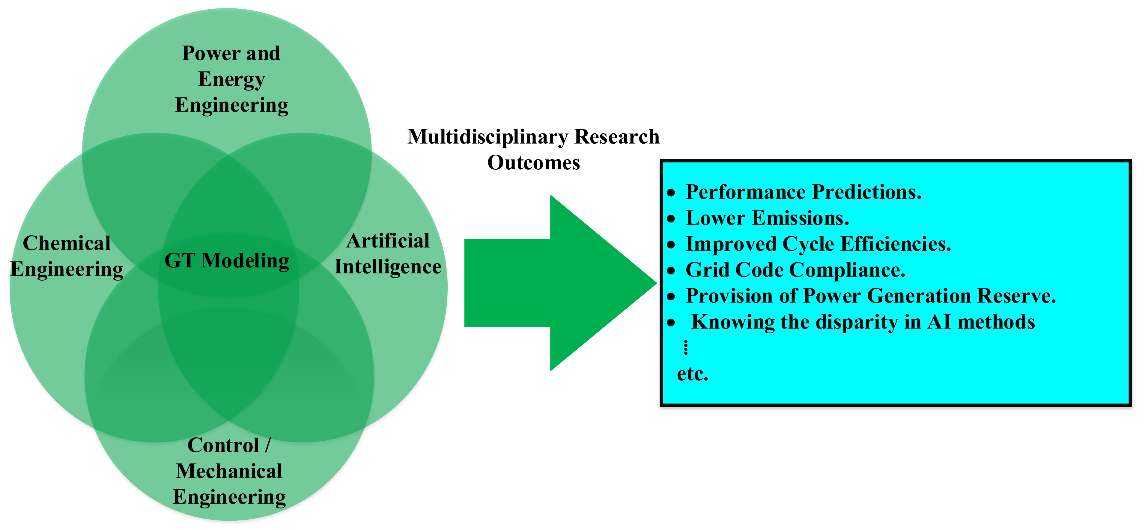
1.1. Aims and Motivations
1.2. Related Work and the Paper Contribution
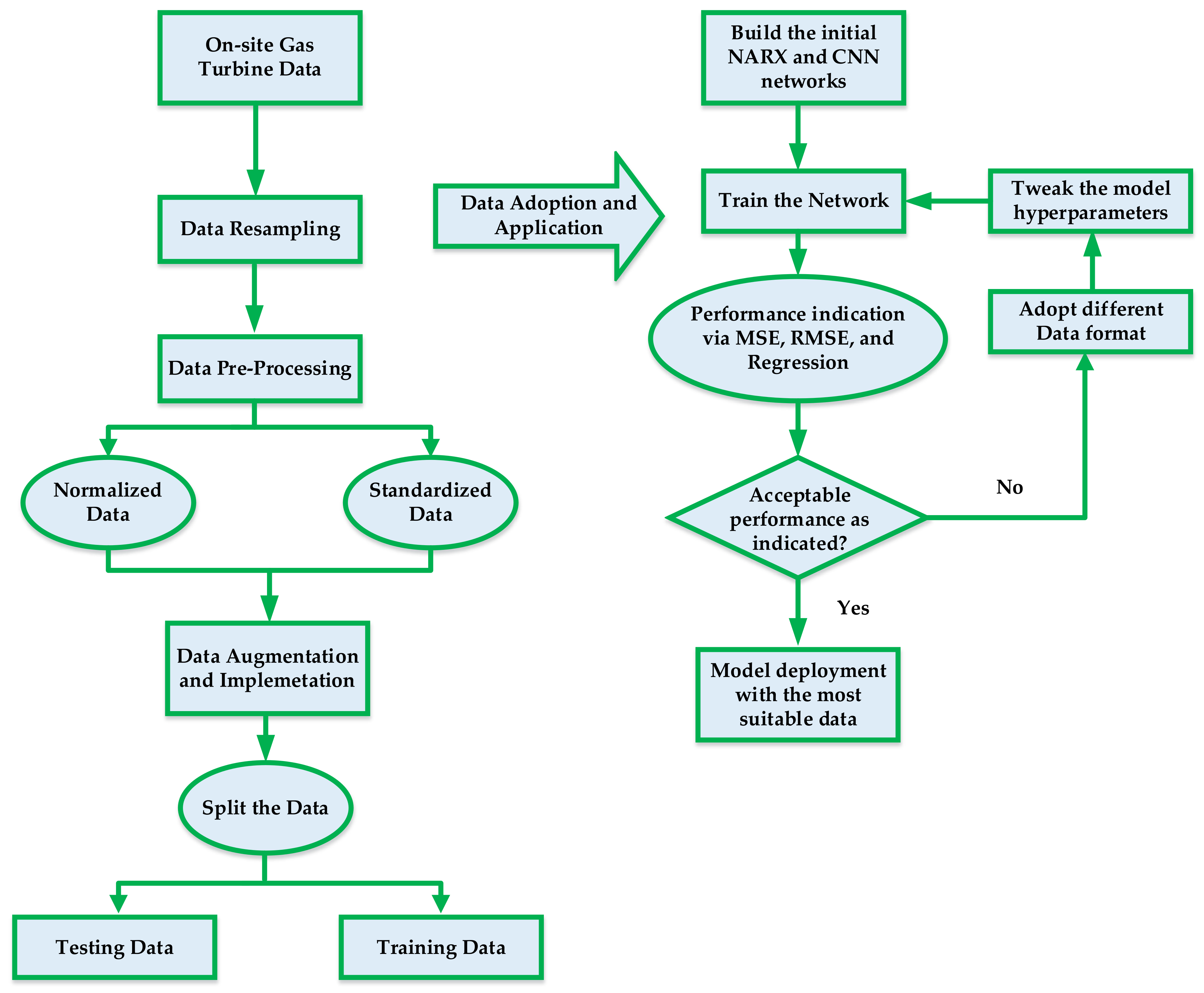
2. Data Curation and Analysis
2.1. Data Normalization
- When equals the minimum, then is 0;
- On the other hand, when is the maximum point in the array, then () is 1;
- However, if is between the minimum and maximum, then () will be between 0 and 1.
2.2. Data Standardization
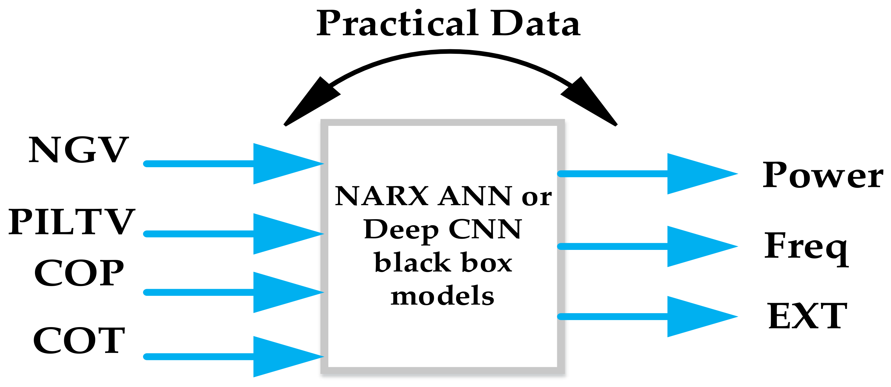
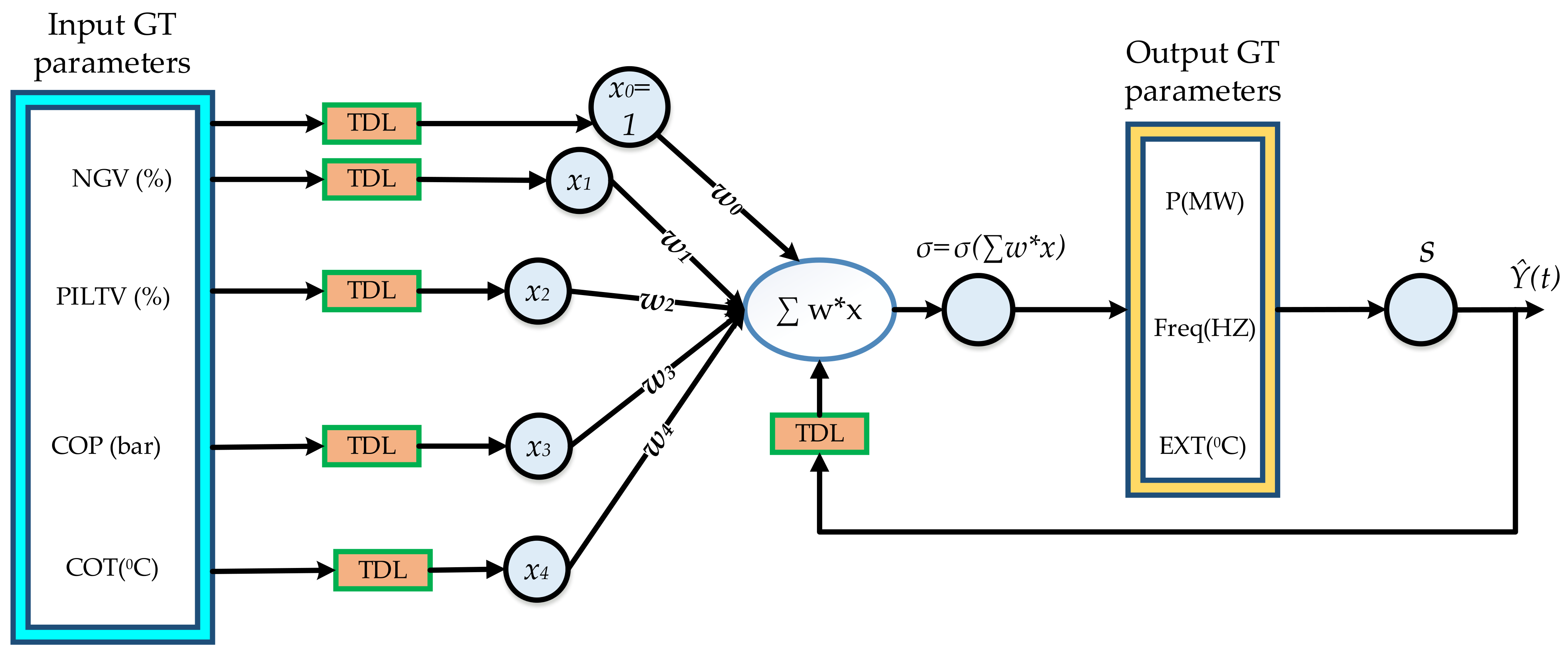
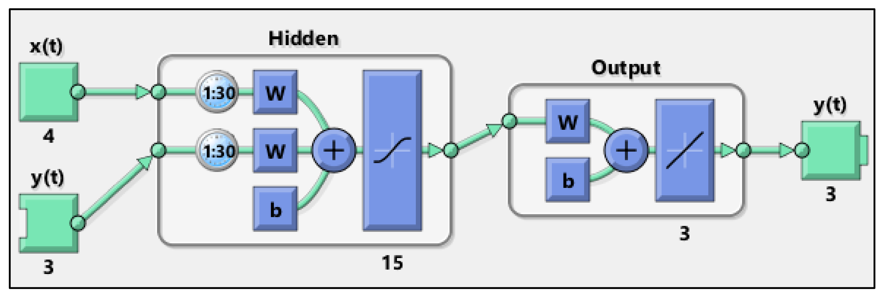
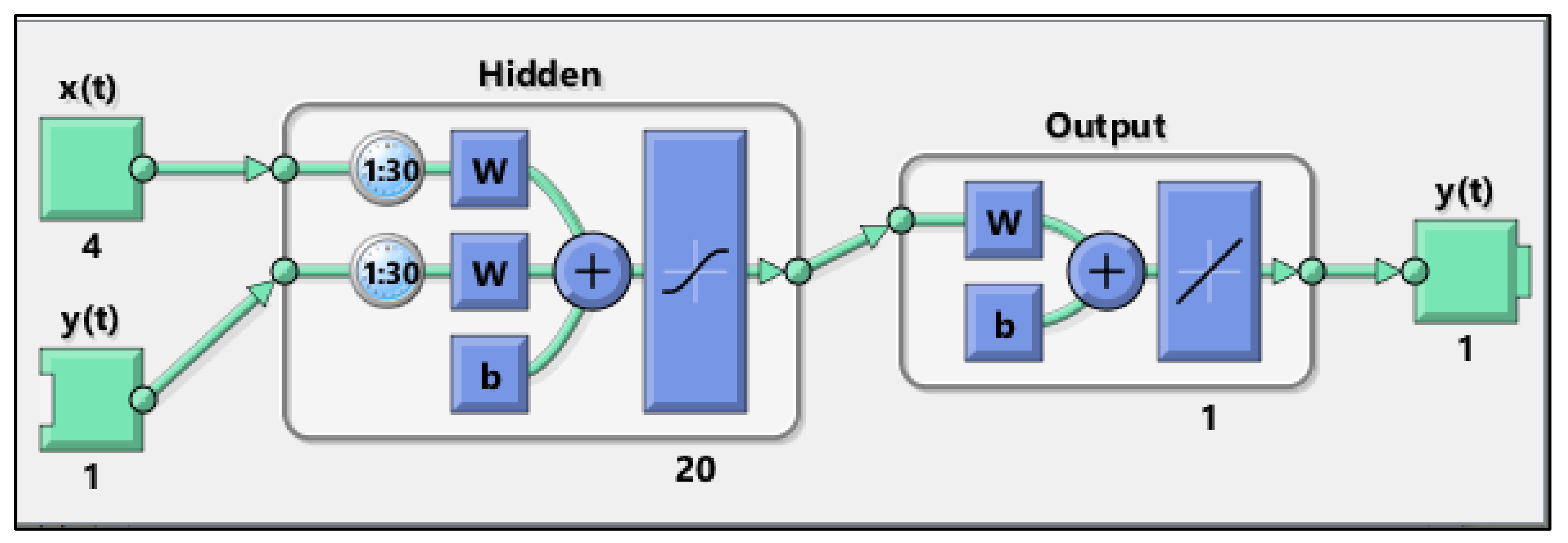
3. The NARX Model Setup
3.1. The MIMO Model
3.2. The Parallel MISO Model
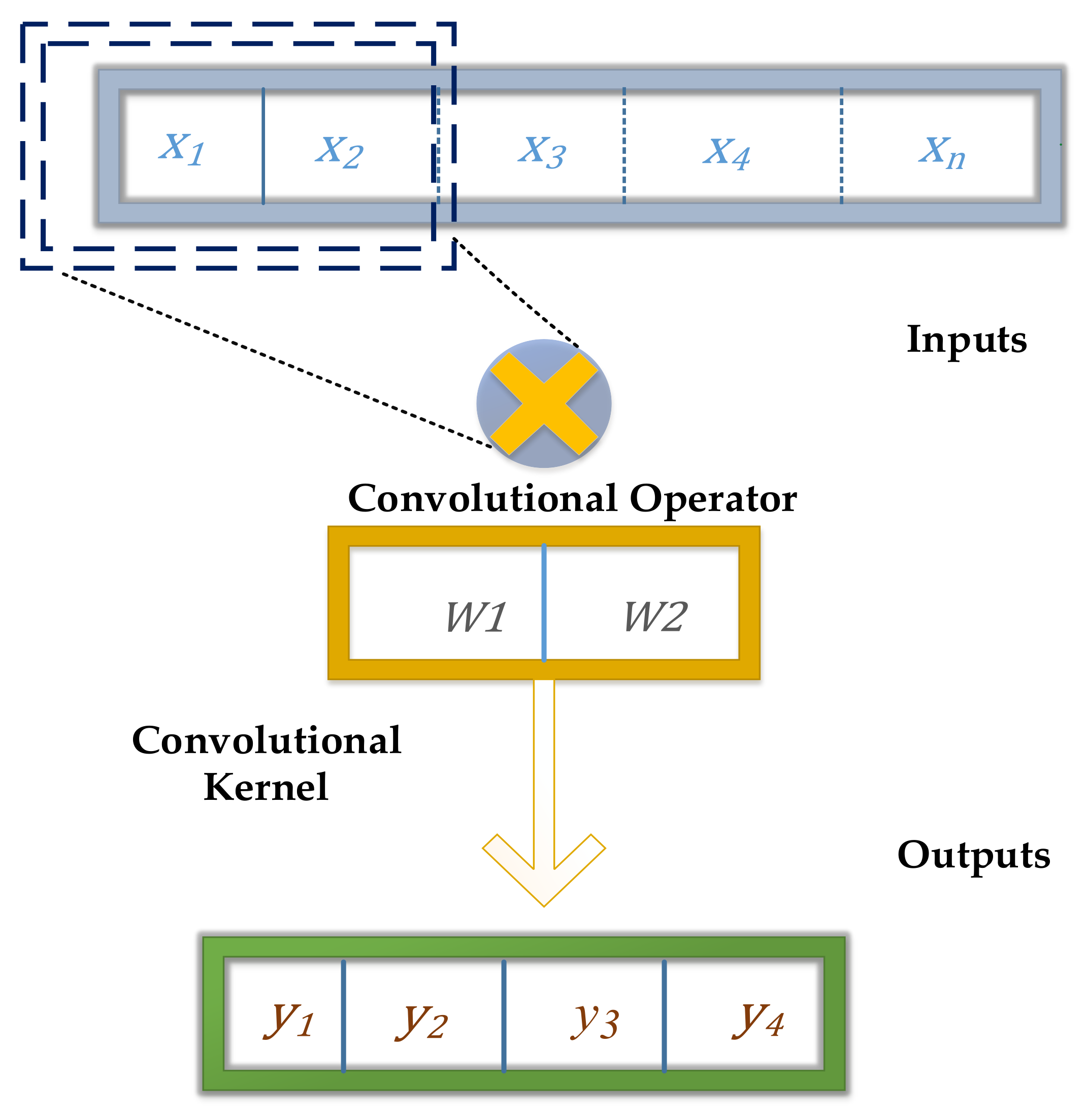
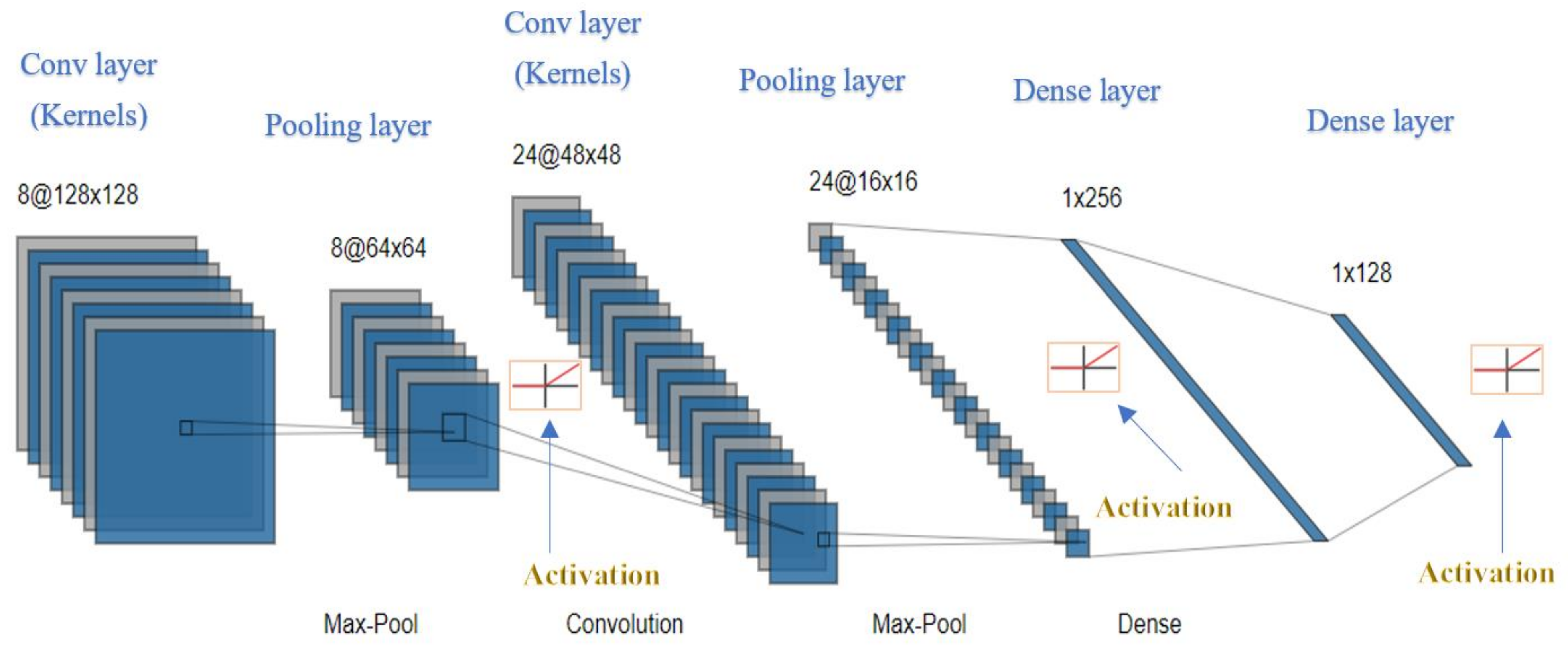
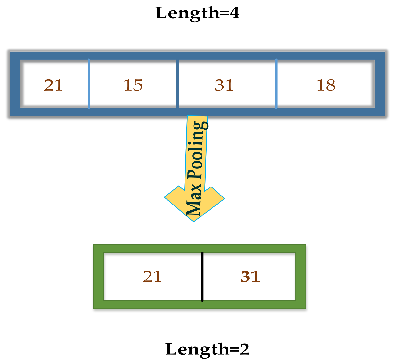
4. The Deep Learning Convolutional Neural Network (CNN) Model Setup

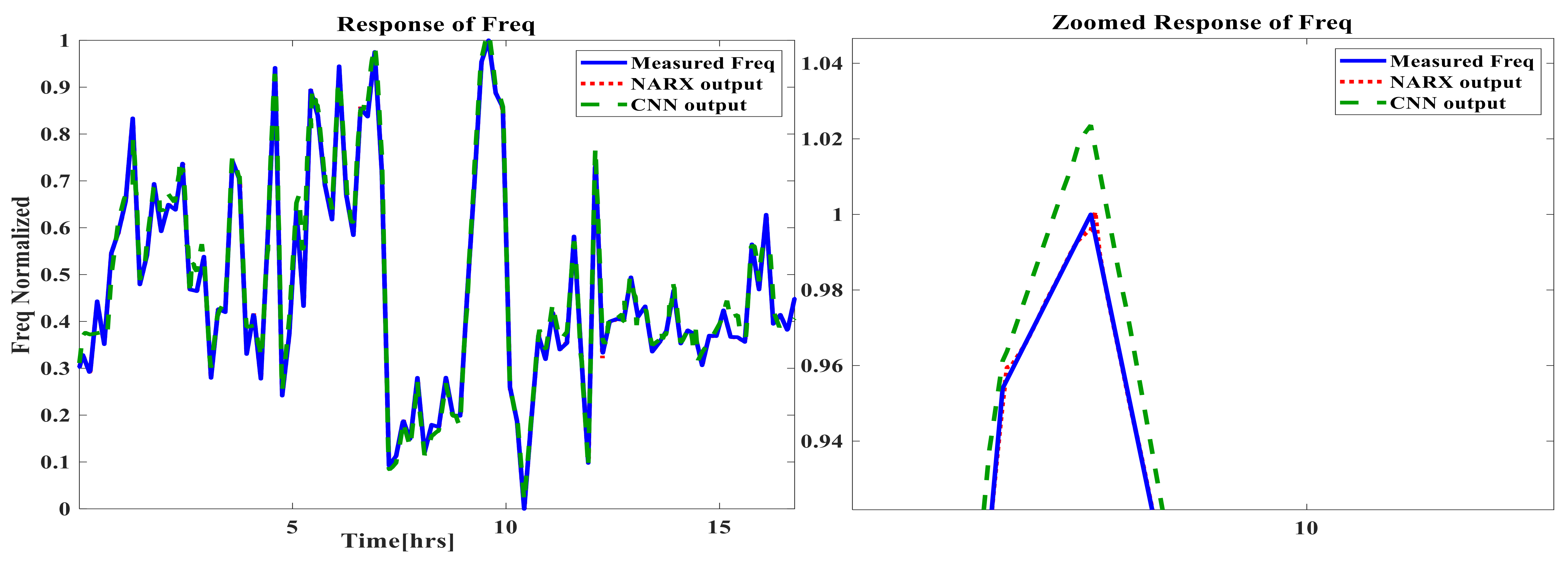
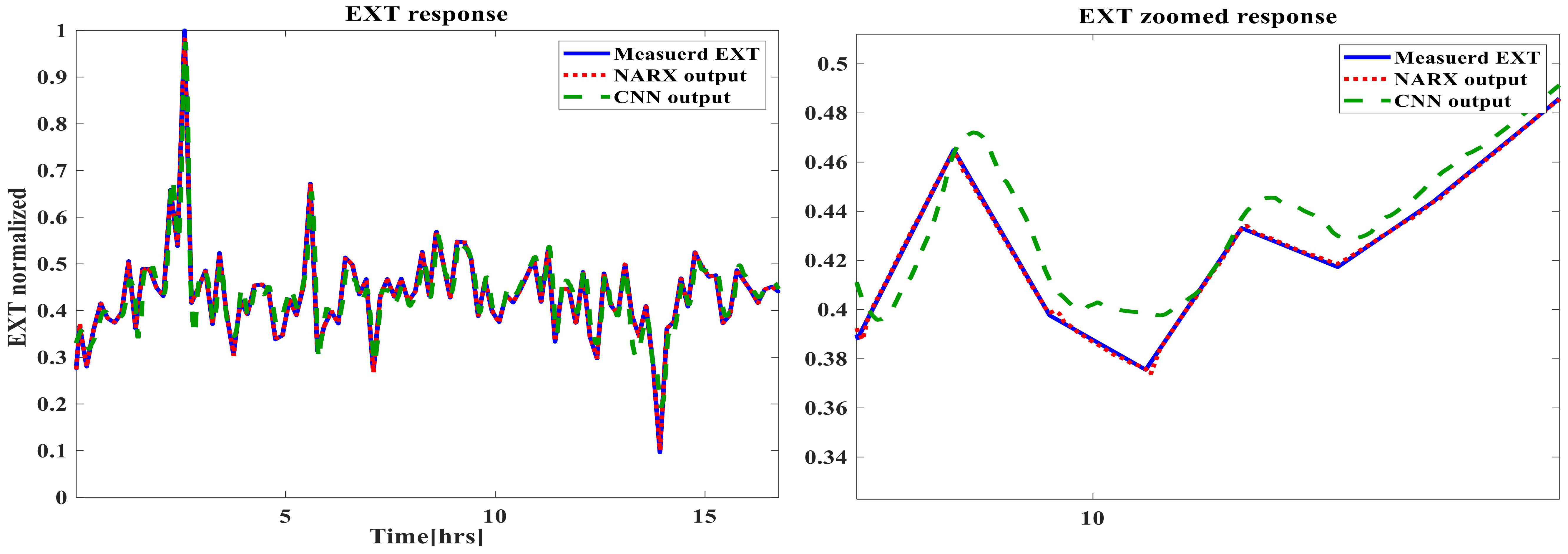
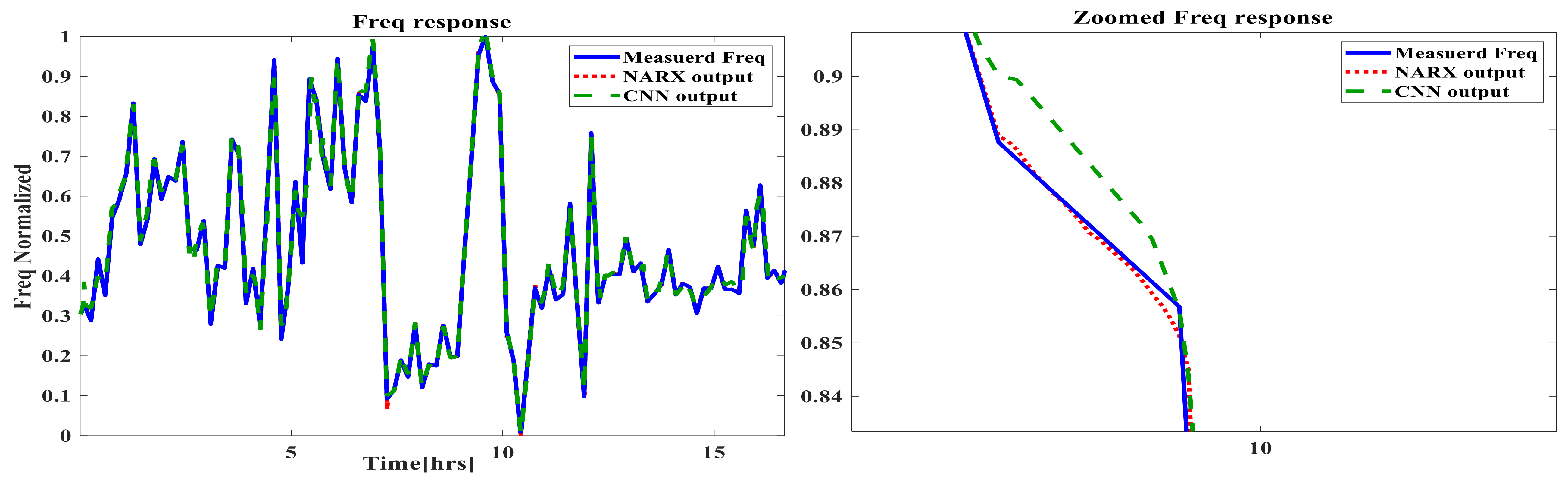
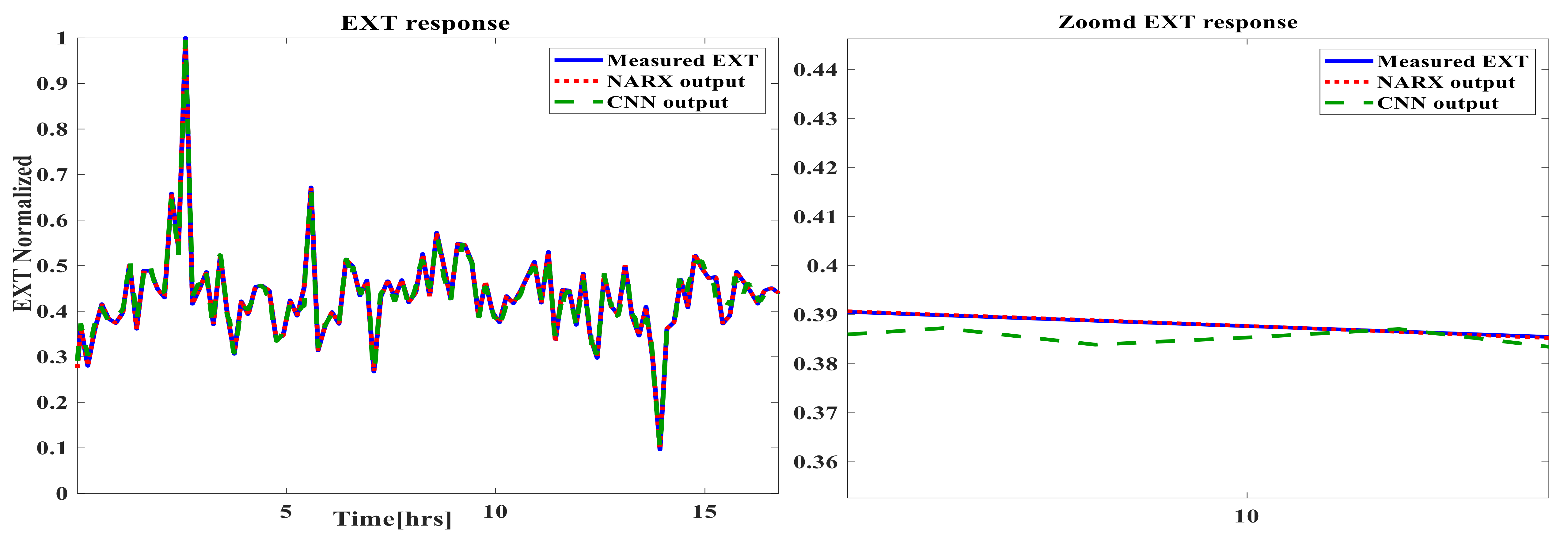
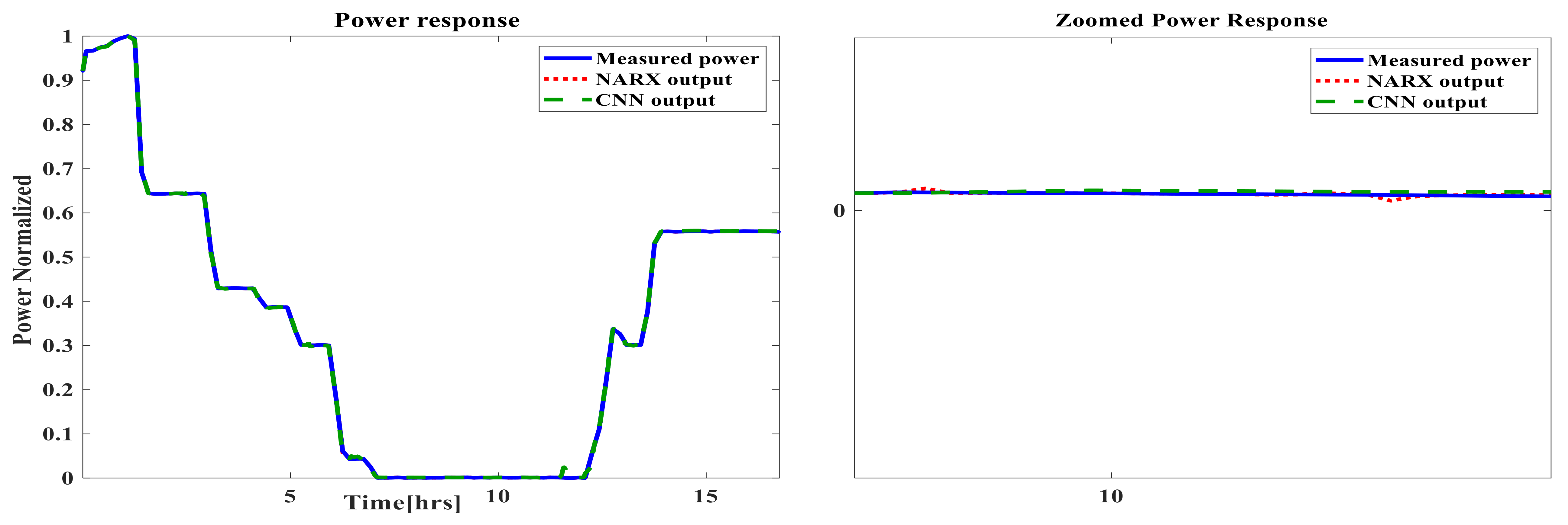
5. Time-Based Simulation Results and Discussion
- Its simplified structure that implicates the direct effect of inputs and outputs; therefore, there are more realistic reflections of the inputs on the outputs;
- The use of feedback delayed outputs as additional inputs, which increase the number of inputs utilized to depict the output more accurately. This important feature has no equivalence in CNN, despite its sophistication in the variety and number of its layers.
6. Conclusions
- It is generally highly recommended to normalize the data of GTs rather than dealing with actual quantities in using ANNs in models;
- The training algorithm of BR outperforms other training algorithms because of its late ultimate termination criteria, unlike other aforementioned earlier ones (LM and SCG);
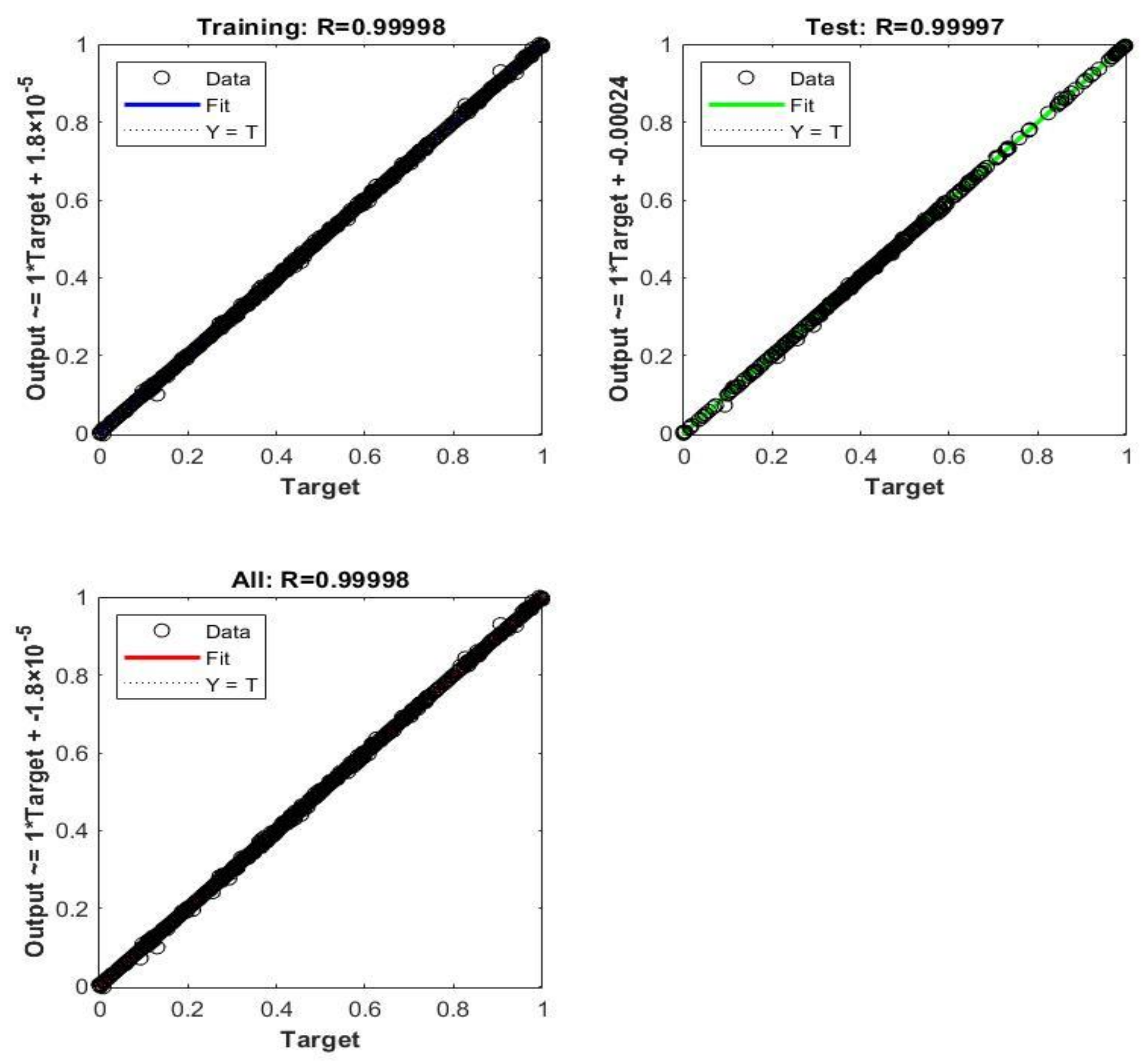
- The prediction capabilities of NARX ANN and CNN for the GTs time-based dynamic performance are satisfactory, with very small negligible errors for both techniques.
- There was a slight superiority of the dynamic NARX type in terms of its accuracy. A new conclusion can be suggested by stating that the main computational reason, which is the feedback delay element in NARX despite the shallow structure, is capable of providing additional information with other direct inputs in order to improve the accuracy over the deep CNN, in which there is no delay feedback element;
- Based on the aforementioned results, deep learning can act as an alternative choice of modeling GTs in real applications, but cannot be a substitutional tool for the shallow dynamic ANN. This is because both have shown successful performances and can be used reliably in real applications;
- Despite the achieved targets of the paper, there are still some deep learning techniques that have not been investigated in the literature; these techniques might have a comparable performance, and this motivates the mentioning of some future research opportunities;
- One of the clearer future trends is to use other deep learning techniques and to compare them appropriately with developed/published ones. This may include the advanced deep recurrent neural network and locally connected neural networks;
- Another possible future outcome is to include the fuel preparation system, especially for biogas firing for such turbines, and the process of (gasification/digestion), in order to quantify the amount of materials used to be converted to biogas and to link those with an enhanced control strategy with new objectives;
- Another feasible future point is designing a supervisory controller for the developed ANN models and applying it to regulate the diffusion and premix modes, together with the objectives of a higher efficiency and lower emissions. A comparative study with other modeling philosophies may be useful, such as physics-based models and other black-box and grey-box models, with emphasis on many performance criteria rather than the mere numeric value of the accuracies.
Author Contributions
Funding
Data Availability Statement
Conflicts of Interest
Abbreviations
| ADGTE | Aero-derivative gas turbine engine |
| ANNs | Artificial neural networks |
| BPNN | Back-propagation Neural Network |
| BR | Bayesian regularization |
| CCGT | Combined cycle gas turbine unit |
| CR | Compression ratio |
| COP | Compressor outlet pressure |
| COT | Compressor outlet temperature |
| CNN | Convolutional neural network |
| EXT | Exhausted temperature |
| FF | Feed-forward |
| Freq | Frequency |
| GT | Gas turbine |
| GE | General electric |
| HRSG | Heat recovery steam generator |
| LM | Levenberg-–Marquardt |
| LSTM | Long short term memory |
| MSE | Mean squared error |
| MIMO | Multi-input multi-output |
| MISO | Multi-input single-output |
| NG | Natural gas |
| NGV | Natural gas control valve position |
| NARX | Nonlinear autoregressive network with exogenous inputs |
| Norm | Normalized data |
| 1D | One-dimension |
| P | Output power |
| PSO | Particle swarm optimization |
| PILTV | Pilot gas valve position |
| R | Regression parameter |
| RMSE | Root mean squared error |
| SCG | Scaled conjugate |
| Stand | Standardized data |
| TDL | Tapped delay line |
References
- Boyce, M.P. Gas Turbine Engineering Handbook; Elsevier: Amsterdam, The Netherlands, 2011. [Google Scholar]
- Rayaprolu, K. Boilers for Power and Process; CRC Press: Boca Raton, FL, USA, 2009. [Google Scholar]
- Mohamed, O.; Wang, J.; Khalil, A.; Limhabrash, M. Predictive control strategy of a gas turbine for improvement of combined cycle power plant dynamic performance and efficiency. SpringerPlus 2016, 5, 501. [Google Scholar] [CrossRef] [PubMed] [Green Version]
- Mohamed, O.; Za’ter, M. Comparative Study Between Three Modeling Approaches for a Gas Turbine Power Generation System. Arab. J. Sci. Eng. 2020, 45, 1803–1820. [Google Scholar] [CrossRef]
- Mohamed, O.K. Progress in Modeling and Control of Gas Turbine Power Generation Systems: A Survey. Energies 2020, 13, 2358. [Google Scholar] [CrossRef]
- Thangavelu, S.K.; Arthanarisamy, M. Experimental investigation on engine performance, emission, and combustion characteristics of a DI CI engine using tyre pyrolysis oil and diesel blends doped with nanoparticles. Environ. Prog. Sustain. Energy 2020, 39, e13321. [Google Scholar] [CrossRef]
- Murugesan, A.; Umarani, C.; Subramanian, R.; Nedunchezhian, N. Bio-diesel as an alternative fuel for diesel engines–A review. Renew. Sustain. Energy Rev. 2009, 13, 653–662. [Google Scholar] [CrossRef]
- Yaqoob, H.; Teoh, Y.H.; Ud Din, Z.; Sabah, N.U.; Jamil, M.A.; Mujtaba, M.A.; Abid, A. The potential of sustainable biogas production from biomass waste for power generation in Pakistan. J. Clean. Prod. 2021, 307, 127250. [Google Scholar] [CrossRef]
- Teoh, Y.H.; How, H.G.; Sher, F.; Le, T.D.; Nguyen, H.T.; Yaqoob, H. Fuel Injection Responses and Particulate Emissions of a CRDI Engine Fueled with Cocos nucifera Biodiesel. Sustainability 2021, 13, 4930. [Google Scholar] [CrossRef]
- Ayanoglu, A.; Yumrutas, R. Production of gasoline and diesel like fuels from waste tire oil by using catalytic pyrolysis. Energy 2016, 103, 456–468. [Google Scholar] [CrossRef]
- Asgari, H. Modelling, Simulation and Control of Gas Turbines Using Artificial Neural Networks. Ph.D. Thesis, University of Canterbury, Christchurch, New Zealand.
- Asgari, H.; Chen, X.; Morini, M.; Pinelli, M.; Sainudiin, R.; Rugerro Spina, P.; Venturini, M. NARX models for simulation of the start-up operation of a single-shaft gas turbine. Appl. Therm. Eng 2016, 93, 368–376. [Google Scholar] [CrossRef]
- Asgari, H.; Ory, E. Prediction of Dynamic Behavior of a Single Shaft Gas Turbine Using NARX Models. In Proceedings of the ASME Turbo Expo 2021: Turbomachinery Technical Conference and Exposition. Volume 6: Ceramics and Ceramic Composites; Coal, Biomass, Hydrogen, and Alternative Fuels; Microturbines, Turbochargers, and Small Turbomachines, Virtual, Online, 7–11 June 2021. V006T19A007. ASME. [Google Scholar]
- Asgari, H.; Ory, E.; Lappalainen, J. Recurrent Neural Network Based Simulation of a Single Shaft Gas Turbine. In Finland Linköping Electronic Conference Proceedings, Proceedings of The 61st SIMS Conference on Simulation and Modelling SIMS, Virtual Conference, 22–24 September 2020; LiU Electronic Press: Linköping, Finland, 2020; Volume 176, pp. 99–106. [Google Scholar] [CrossRef]
- Ibrahem, I.M.A. A Nonlinear Neural Network-Based Model Predictive Control for Industrial Gas Turbine. Ph.D. Thesis, Université Du Québec, Quebec, QC, Canada, 2020. [Google Scholar]
- Rashid, M.; Kamal, K.; Zafar, T.; Sheikh, A.; Shah, A.; Mathavan, S. Energy prediction of a combined cycle power plant using a particle swarm optimization trained feed-forward neural network. In Proceedings of the IEEE International Conference on Mechanical Engineering Automation and Control Systems, Tomsk, Russia, 1–4 December 2015; pp. 1–5. [Google Scholar]
- Rahmoune, M.B.; Hafaifa, A.; Kouzou, A.; Chen, X.; Chaibet, A. Gas turbine monitoring using neural network dynamic nonlinear autoregressive with external exogenous input modelling. Math. Comput. Simul. 2021, 179, 23–47. [Google Scholar] [CrossRef]
- Cao, Q.; Chen, S.; Zheng, Y.; Ding, Y.; Tang, Y.; Huang, Q.; Wang, K.; Xiang, W. Classification and prediction of gas turbine gas path degradation based on deep neural networks. Int. J. Energy Res. 2021, 45, 10513–10526. [Google Scholar] [CrossRef]
- Bulit in’s Expert Contributor Network, Gradient Descent: An Introduction to 1 of Machine Learning’s Most Popular Algorithms, Built in Beta. 2021. Available online: https://builtin.com/data-science/gradient-descent. (accessed on 21 October 2021).
- Ng, A.; Bensouda Mourri, Y.; Katanforoosh, K. DeepLearning.AI, Coursera. 2020. Available online: https://www.coursera.org/learn/deep-neural-network (accessed on 27 December 2021).
- Bhandari, A. Feature Scaling for Machine Learning: Understanding the Difference Between Normalization vs. Standardization. Analytics Vidhya. 2020. Available online: https://www.analyticsvidhya.com/blog/2020/04/feature-scaling-machine-learning-normalization-standardization/ (accessed on 27 December 2021).
- Liu, Q.; Wei, C.; Huosheng, H.; Quingyuan, Z.; Zhixiang, X. An Optimal NARX Neural Network Identification Model for a Magnetorheological Damper With Force-Distortion Behavior. Front. Mater. 2020, 7, 10. [Google Scholar] [CrossRef]
- Markova, M. Foreign Exchange Rate Forecasting by Artificial Neural Networks. AIP Conf. Proc. 2019, 2164, 060010. [Google Scholar] [CrossRef]
- Bai, M.; Yang, X.; Liu, J.; Liu, J.; Yu, D. Convolutional neural network-based deep transfer learning for fault detection of gas turbine combustion chambers. Appl. Energy. 2021, 302, 117509. [Google Scholar] [CrossRef]
- Wunsch, A.; Liesch, T.; Broda, S. Groundwater Level Forecasting with Artificial Neural Networks: A Comparison of LSTM, CNN and NARX. Hydrol. Earth Syst. Sci. 2021, 25, 1671–1687. [Google Scholar] [CrossRef]
- Ragab, M.G.; Abdulkadir, S.J.; Aziz, N.; Al-Tashi, Q.; Alyousifi, Y.; Alhussian, H.; Alqushaibi, A. A Novel One-Dimensional CNN with Exponential Adaptive Gradients for Air Pollution Index Prediction. Sustainability 2020, 12, 10090. [Google Scholar] [CrossRef]
- Schmidhuber, J. Deep learning in neural networks: An overview. Neural Netw. 2015, 61, 85–117. [Google Scholar] [CrossRef] [PubMed] [Green Version]
- Wang, S.; Chen, H. A novel deep learning method for the classification of power quality disturbances using deep convolutional neural network. Appl. Energy 2019, 235, 1126–1140. [Google Scholar] [CrossRef]


| Variable | Abbreviation | Unit | Actual Operational Range |
|---|---|---|---|
| Pilot gas valve position Natural gas control valve position Compressor outlet pressure Compressor outlet temperature | PILTV NGV COP COT | % % bar °C | [41.06–44.79%] [27.18–39.45%] [11.45–16.75] [366.5–439.90] |
| Variable | Abbreviation | Unit | Actual Operational Range |
|---|---|---|---|
| Output power Frequency Exhausted temperature | P Freq EXT | MW Hz | [241.57–124.89] [49.91–50.14] [558.72–559.47] |
| Hidden Layer Neurons | Time Delay | Training Algorithm | Data Format | Performance Average MSE | Regression | ||||
|---|---|---|---|---|---|---|---|---|---|
| Training | Validation | Test | Training | Validation | Test | ||||
| 5 | 2 | LM | Actual | 3.4998 × 10⁻⁶ | 4.3858 × 10⁻⁶ | 6.1132 × 10⁻⁶ | 0.99997 | 0.99996 | 0.99994 |
| 11 | 15 | LM | Stand | 3.1147 × 10⁻⁶ | 4.2107 × 10⁻⁶ | 8.6999 × 10⁻⁶ | 0.99998 | 0.99996 | 0.99991 |
| 20 | 20 | LM | Norm | 3.4393 × 10⁻⁶ | 4.5559 × 10⁻⁶ | 3.8095 × 10⁻⁶ | 0.99997 | 0.99995 | 0.99996 |
| 11 | 15 | BR | Stand | 2.3191 × 10⁻⁶ | 6.050 × 10⁻⁶ | 0.99998 | 0.99994 | ||
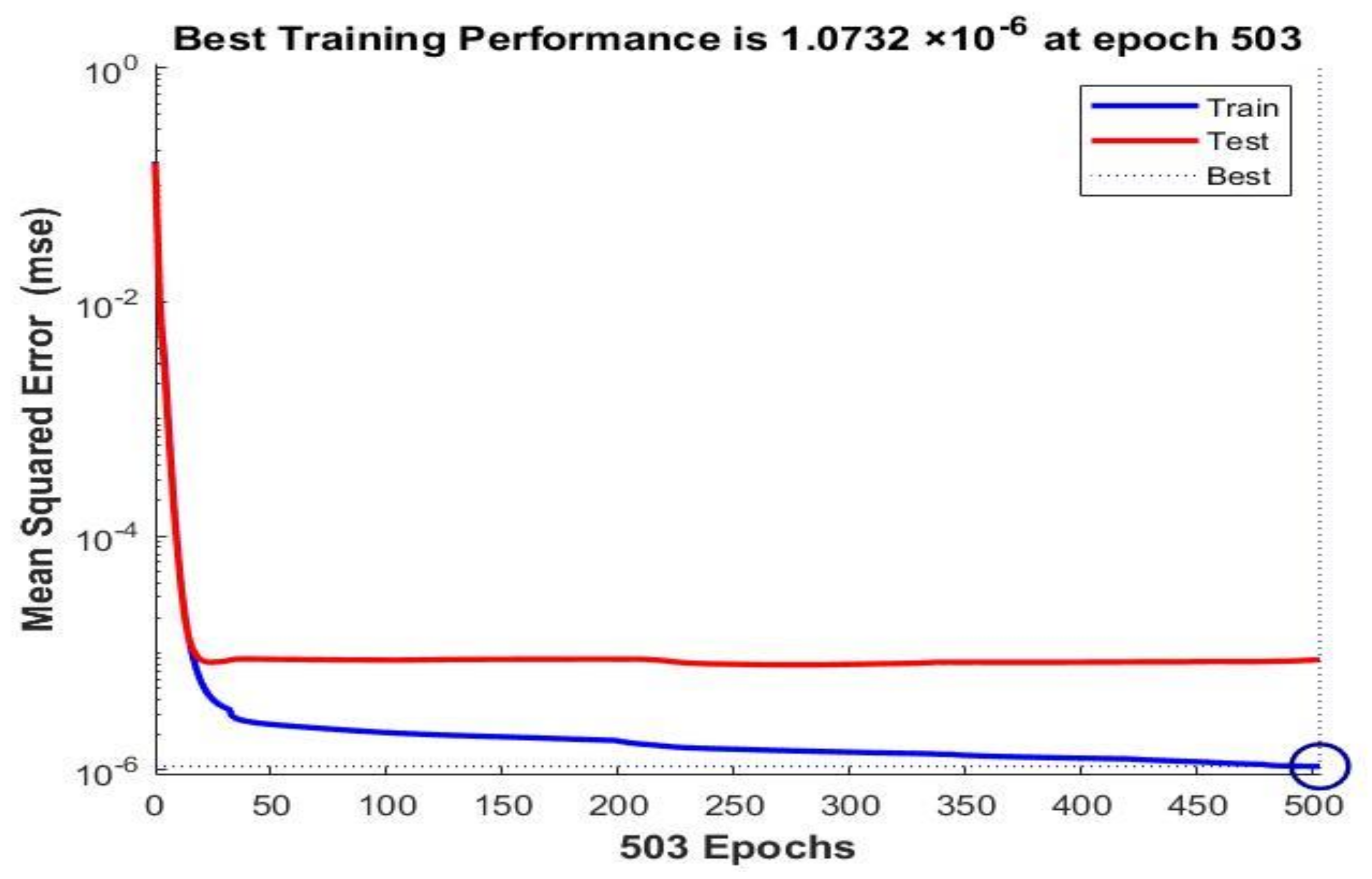
| 15 | 30 | BR | Norm | 1.0732 × 10⁻⁶ | 3.2062 × 10⁻⁶ | 0.99998 | 0.99997 | ||
| 20 | 20 | BR | Norm | 2.7990 × 10⁻⁶ | 3.2469 × 10⁻⁶ | 0.99997 | 0.99996 | ||
| 9 | 5 | SCG | Actual | 4.5996 × 10⁻⁵ | 4.4098 × 10⁻⁵ | 3.1814 × 10⁻⁵ | 0.99993 | 0.99993 | 0.99993 |
| 15 | 15 | SCG | Norm | 1.4164 × 10⁻⁴ | 1.6761 × 10⁻⁴ | 2.6512 × 10⁻⁴ | 0.99992 | 0.99994 | 0.99993 |
| Hidden Layer Neurons | Time Delay | Training Algorithm | Data Format | Performance MSE | Regression | ||||
|---|---|---|---|---|---|---|---|---|---|
| Training | Validation | Test | Training | Validation | Test | ||||
| 9 | 5 | LM | Actual | 1.9266 × 10⁻⁷ | 2.0124 × 10⁻⁷ | 3.2844 × 10⁻⁶ | 0.99997 | 0.99996 | 0.99997 |
| 11 | 15 | LM | Stand | 2.8425 × 10⁻⁷ | 4.3205 × 10⁻⁷ | 3.4621 × 10⁻⁶ | 0.99996 | 0.99997 | 0.99991 |
| 20 | 30 | LM | Norm | 2.6179 × 10⁻⁷ | 3.0105 × 10⁻⁷ | 1.2145 × 10⁻⁶ | 0.99996 | 0.99997 | 0.99996 |
| 9 | 5 | BR | Actual | 2.5613 × 10⁻⁸ | 6.7436 × 10⁻⁶ | 0.99996 | 0.99989 | ||
| 11 | 15 | BR | Stand | 1.7642 × 10⁻⁸ | 3.3149 × 10⁻⁷ | 1 | 1 | ||
| 15 | 25 | BR | Norm | 1.4258 × 10⁻⁸ | 1.4642 × 10⁻⁷ | 1 | 1 | ||
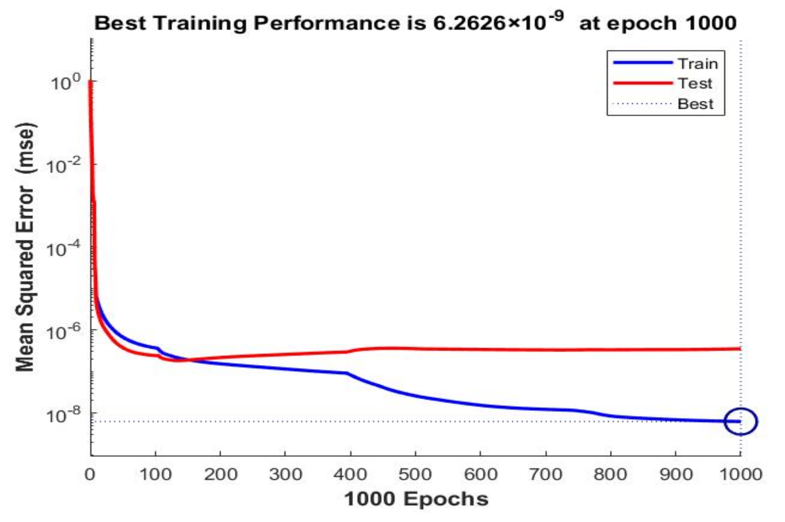
| 20 | 30 | BR | Norm | 6.2626 × 10⁻⁹ | 3.4983 × 10⁻⁷ | 1 | 1 | ||
| 9 | 5 | SCG | Actual | 4.4996 × 10⁻⁵ | 4.2032 × 10⁻⁵ | 2.3214 × 10⁻⁵ | 0.99272 | 0.99097 | 0.99505 |
| 11 | 15 | SCG | Stand | 1.5093 × 10⁻⁴ | 2.6054 × 10⁻⁴ | 2.4232 × 10⁻⁴ | 0.99562 | 0.99341 | 0.99598 |
| 15 | 25 | SCG | Norm | 1.3164 × 10⁻⁴ | 2.7791 × 10⁻⁴ | 1.6512 × 10⁻⁴ | 0.95759 | 0.94021 | 0.95058 |
| Hidden Layer Neurons | Time Delay | Training Algorithm | Data Format | Performance MSE | Regression | ||||
|---|---|---|---|---|---|---|---|---|---|
| Training | Validation | Test | Training | Validation | Test | ||||
| 9 | 5 | LM | Actual | 6.0188 × 10⁻⁶ | 2.0124 × 10⁻⁷ | 3.2844 × 10⁻⁶ | 0.99997 | 0.99996 | 0.99997 |
| 11 | 15 | LM | Stand | 7.5393 × 10⁻⁶ | 4.3205 × 10⁻⁷ | 3.4621 × 10⁻⁶ | 0.99996 | 0.99997 | 0.99991 |
| 20 | 30 | LM | Norm | 8.4340 × 10⁻⁶ | 3.0105 × 10⁻⁷ | 1.2145 × 10⁻⁶ | 0.99996 | 0.99997 | 0.99996 |
| 9 | 5 | BR | Actual | 3.7643 × 10⁻⁶ | 6.7436 × 10⁻⁶ | 0.99996 | 0.99989 | ||
| 11 | 15 | BR | Stand | 3.7362 × 10⁻⁶ | 3.3149 × 10⁻⁷ | 1 | 1 | ||
| 15 | 25 | BR | Norm | 1.5820 × 10⁻⁶ | 1.4642 × 10⁻⁷ | 1 | 1 | ||
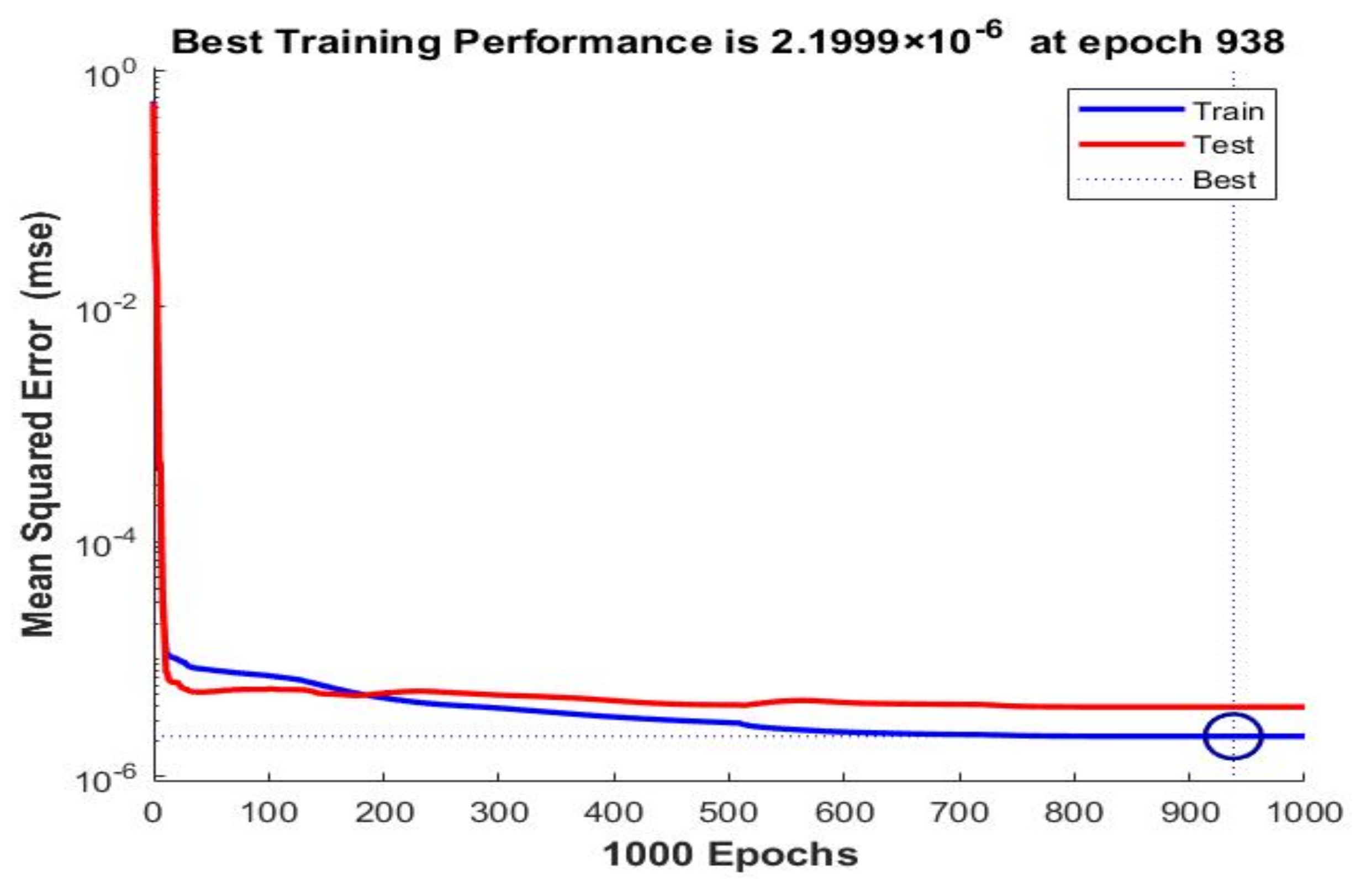
| 20 | 30 | BR | Norm | 2.1999 × 10⁻⁶ | 3.4983 × 10⁻⁷ | 1 | 1 | ||
| 5 | 2 | SCG | Actual | 2.4112 × 10⁻⁴ | 3.1053 × 10⁻⁴ | 2.2242 × 10⁻⁴ | 0.99332 | 0.99379 | 0.99023 |
| 11 | 15 | SCG | Stand | 2.4386 × 10⁻⁴ | 2.6054 × 10⁻⁴ | 2.4232 × 10⁻⁴ | 0.99341 | 0.99341 | 0.99588 |
| 15 | 25 | SCG | Norm | 3.4042 × 10⁻⁵ | 2.7791 × 10⁻⁴ | 1.6512 × 10⁻⁴ | 0.95658 | 0.96020 | 0.95038 |
| Hidden Layer Neurons | Time Delay | Training Algorithm | Data Format | Performance MSE | Regression | ||||
|---|---|---|---|---|---|---|---|---|---|
| Training | Validation | Test | Training | Validation | Test | ||||
| 5 | 2 | LM | Actual | 1.8337 × 10⁻⁶ | 1.3246 × 10⁻⁶ | 6.1132 × 10⁻⁶ | 0.99997 | 0.99996 | 0.99994 |
| 20 | 30 | LM | Norm | 1.8947 × 10⁻⁶ | 1.5678 × 10⁻⁶ | 3.8095 × 10⁻⁶ | 0.99997 | 0.99995 | 0.99996 |
| 5 | 2 | BR | Actual | 1.4468 × 10⁻⁶ | 2.7617 × 10⁻⁶ | 0.99990 | 0.99979 | ||
| 15 | 25 | BR | Norm | 4.2333 × 10⁻⁶ | 2.9041 × 10⁻⁶ | 0.99998 | 0.99997 | ||
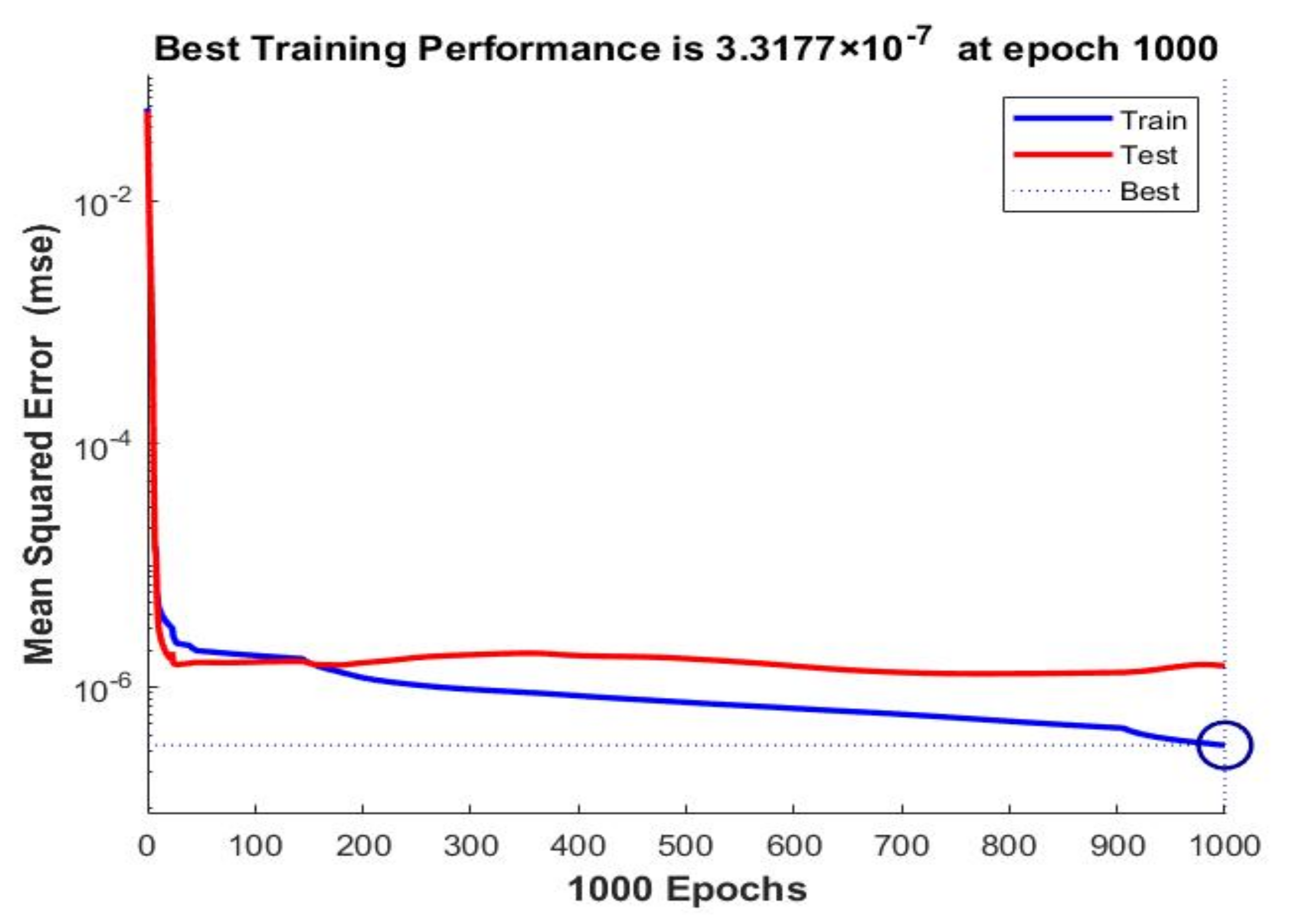
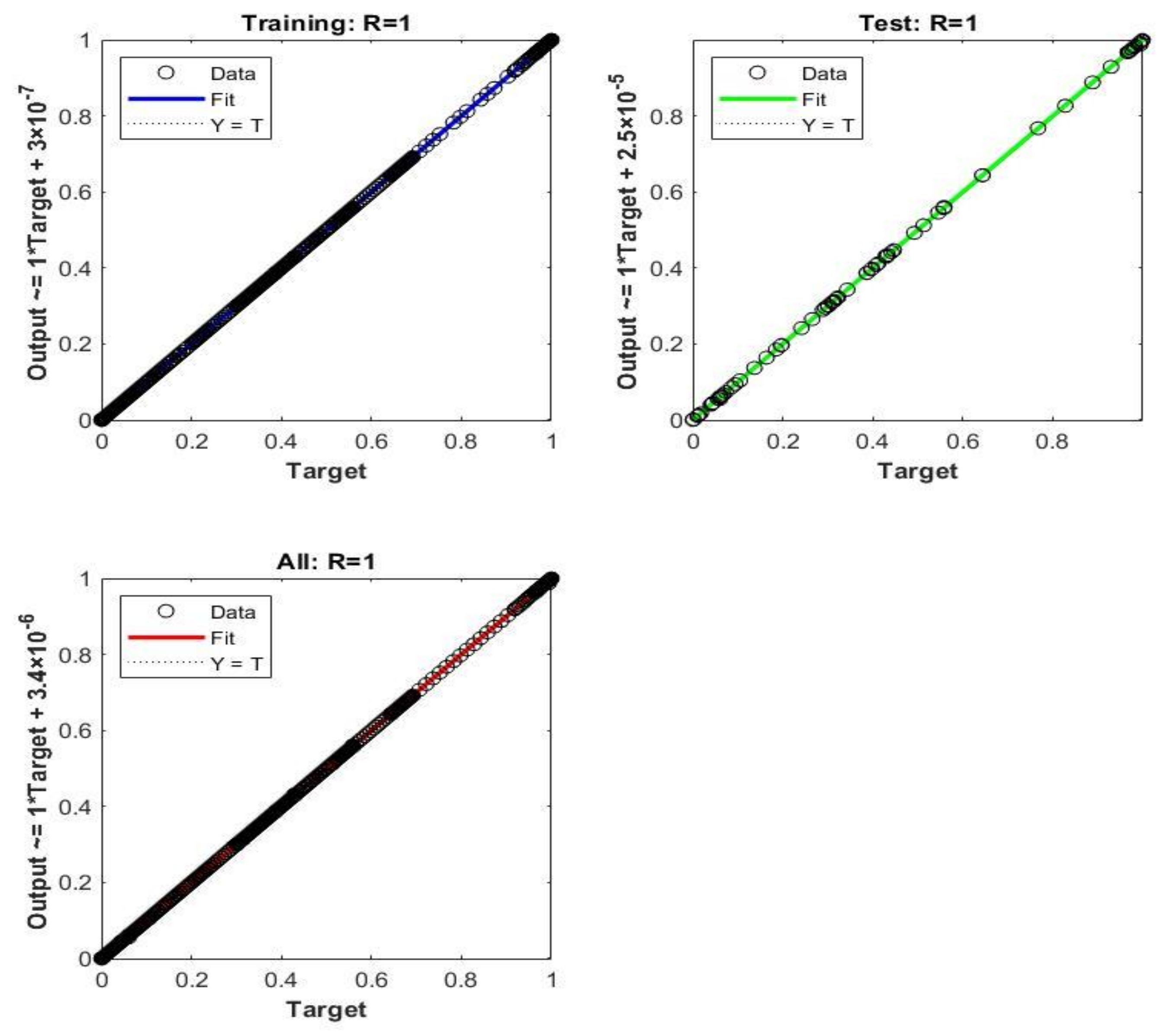
| 20 | 30 | BR | Norm | 3.3177 × 10⁻⁷ | 1.4889 × 10⁻⁶ | 1 | 1 | ||
| 9 | 5 | SCG | Actual | 1.1165 × 10⁻⁴ | 1.2062 × 10⁻⁴ | 2.1814 × 10⁻⁴ | 0.99219 | 0.99002 | 0.99108 |
| 10 | 10 | SCG | Stand | 7.8369 × 10⁻⁵ | 9.0913 × 10⁻⁵ | 7.1945 × 10⁻⁵ | 0.99444 | 0.99215 | 0.99519 |
| 15 | 25 | SCG | Norm | 7.4106 × 10⁻⁴ | 6.9733 × 10⁻⁴ | 7.01950 × 10⁻⁴ | 0.94648 | 0.94070 | 0.94048 |
| Parallel MISO CNN | MIMO CNN All Outputs | ||||||
|---|---|---|---|---|---|---|---|
| Normalized EXT | Normalized Freq | Normalized P | |||||
| Learning Rate | Average MSE | Learning Rate | Average MSE | Learning Rate | Average MSE | Learning Rate | Average MSE |
| 1 | 0.1000023029 | 1 | 0.0486324 | 1 | 0.1000023029 | 1 | 0.0623 |
| 1 × 10⁻² | 0.0009281756 | 1 × 10⁻¹ | 0.0461746 | 1 × 10⁻² | 0.0000920723 | 1 × 10⁻² | 0.0010 |
| 1 × 10⁻³ | 0.0000754316 | 1 × 10⁻³ | 0.0059033 | 1 × 10⁻³ | 0.0000502320 | 1 × 10⁻³ | 0.0012 |
| 1 × 10⁻⁵ | 0.0009873912 | 1 × 10⁻⁶ | 0.0052704 | 1 × 10⁻⁵ | 0.0008763900 | 1 × 10⁻⁵ | 0.0142 |
| 1 × 10⁻⁷ | 0.3573216283 | 1 × 10⁻⁹ | 0.2094497 | 1 × 10⁻⁷ | 0.1232704280 | 1 × 10⁻⁷ | 0.1450 |
| 3 × 10⁻¹ | 0.0987941528 | 3 × 10⁻³ | 0.0015080 | 3 × 10⁻¹ | 0.0957923018 | 3 × 10⁻¹ | 0.0616 |
| 3 × 10⁻² | 0.0041973211 | 4 × 10⁻³ | 0.0018637 | 3 × 10⁻² | 0.0011962601 | 3 × 10⁻² | 0.00412842 |
| 3 × 10⁻³ | 0.0000452316 | 5 × 10⁻³ | 0.0026439 | 3 × 10⁻³ | 0.0000384926 | 3 × 10⁻³ | 0.00074576 |
| 3 × 10⁻⁵ | 0.0004128134 | 5 × 10⁻⁴ | 0.0022009 | 3 × 10⁻⁵ | 0.0003279034 | 1 | 0.01075099 |
| 3 × 10⁻⁷ | 0.0083392732 | 6 × 10⁻³ | 0.0035000 | 3 × 10⁻⁷ | 0.0040356721 | 1 × 10⁻² | 0.03599427 |
| Parallel MISO CNN | MIMO CNN | |||
|---|---|---|---|---|
| CNN Adjustable Design Parameter | Normalized EXT Performance | Normalized Freq Performance | Normalized Power Performance | All Outputs |
| No. of convolutional layers | 3 | 2 | 3 | 3 |
| Filter size for each convolutional layer | 2 | 2 | 2 | 2 |
| No. of filters in the convolutional layer | 64_32_256 | 100_200 | 64_32_256 | 256_32_32 |
| No. of hidden layers | 1 | 1 | 1 | 1 |
| No. of neurons in the hidden layer | 70 | 100 | 64 | 70 |
| Max-pooling layers | 2 | 2 | 2 | 2 |
| Filter size in each max-pooling layer | 2 | 2 | 2 | 2 |
| Final MSE | 8.6124826 × 10⁻⁶ | 2.9210 × 10⁻⁴ | 8.3504346 × 10⁻⁶ | 1.6581 × 10⁻⁴ |
Publisher’s Note: MDPI stays neutral with regard to jurisdictional claims in published maps and institutional affiliations. |
© 2022 by the authors. Licensee MDPI, Basel, Switzerland. This article is an open access article distributed under the terms and conditions of the Creative Commons Attribution (CC BY) license (https://creativecommons.org/licenses/by/4.0/).
Share and Cite
Alsarayreh, M.; Mohamed, O.; Matar, M. Modeling a Practical Dual-Fuel Gas Turbine Power Generation System Using Dynamic Neural Network and Deep Learning. Sustainability 2022, 14, 870. https://doi.org/10.3390/su14020870
Alsarayreh M, Mohamed O, Matar M. Modeling a Practical Dual-Fuel Gas Turbine Power Generation System Using Dynamic Neural Network and Deep Learning. Sustainability. 2022; 14(2):870. https://doi.org/10.3390/su14020870
Chicago/Turabian StyleAlsarayreh, Mohammad, Omar Mohamed, and Mustafa Matar. 2022. "Modeling a Practical Dual-Fuel Gas Turbine Power Generation System Using Dynamic Neural Network and Deep Learning" Sustainability 14, no. 2: 870. https://doi.org/10.3390/su14020870
APA StyleAlsarayreh, M., Mohamed, O., & Matar, M. (2022). Modeling a Practical Dual-Fuel Gas Turbine Power Generation System Using Dynamic Neural Network and Deep Learning. Sustainability, 14(2), 870. https://doi.org/10.3390/su14020870