The Impact of Vehicle Ownership on Carbon Emissions in the Transportation Sector

Abstract

As one of the important sources of carbon emissions, the transportation industry should be given attention. This study investigates the relationship between vehicle ownership, economic growth, and environmental pressure on the Chongqing transportation industry (CQTI) based on CQTI data, then constructs a comprehensive regression model and couples the EKC curve and Tapio model for integrated analysis, and finally constructs a LEAP-Chongqing model to forecast CQTI from multiple perspectives. The innovations are that the multi-model examines the effects of different variables and has a better classification of transportation modes in scenario simulation. The results show that: (1) there is an inverse N-shaped relationship between car ownership, economic growth, and environmental pressure of CQTI; (2) every 1% of transportation output, urbanization rate, or car ownership will cause 0.769%, 0.111%, and 0.096% of carbon emission change, respectively; (3) gasoline, diesel and aviation kerosene consumption account for 80–90%, private cars cause 41–52% of carbon emissions, and the energy structure and transportation structure of CQTI are unreasonable; (4) the results of a multi-scenario simulation show that the energy saving and emission reduction effect of a single policy is not satisfactory, and the integration of energy saving and emission reduction measures should be strengthened.

1. Introduction

Climate change caused by global warming has become one of the most significant challenges to human development in the new century, and China, the world’s largest carbon emitter [1], has made it an important task to promote sustainable human development. In China, transportation is one of the most important sources of carbon emissions [2]. Therefore, the transportation sector is important in achieving carbon peaking and carbon neutrality in China.

The latest data show that car ownership in China exceeded 300 million marks [3], which will continue to grow as living standards improve. Therefore, more and more studies have started focusing on the relationship between factors such as car ownership, urbanization, and transportation development. They have examined their impact on the environment and regional economic development through different methods and models. A study by Huang [4] et al. on China, the United States, and Japan showed that China lags behind Japan and the United States in formulating and implementing environmental policies. Kharbach [5] et al. explored the Moroccan transport sector and found that population growth and increased household car ownership are essential factors in the growth of carbon emissions. Wang [6] and Xu [7] et al. used the Tapio and dynamic nonparametric weighted regression model to study the Chinese transportation industry, respectively, and the results showed poor decoupling between economic development and carbon emissions in this industry. Gambhir [8] conducted a scenario simulation of the transportation sector in China using the Long-range Energy Alternatives Planning System (LEAP) and concluded that private cars and heavy trucks constitute the majority of the future emission reduction potential. Zhao [9] et al. showed that the increase in car ownership harms urban transport development. Zhu [10] et al. studied the transportation sector in Shaanxi Province and found that regional economic growth was a contributing factor to carbon emissions, while lower energy intensity had a suppressive effect. Pang [11] studied Lanzhou City and found that clean energy and vehicle restructuring are effective measures to reduce carbon emissions. Some other studies have shown that urban development, transportation composition structure, and vehicle replacement rates are the most influential parameters for developing carbon emission reduction policies [12,13]. Some results from least partial squares (PLS) studies suggest that the increase in private cars worsens air quality and increases carbon emissions [14] and that there is a growing desire to purchase electric cars [15]. Meanwhile, some of the studies in policy suggest that using alternative fuels and upgrading energy application technologies will significantly control carbon emissions [16,17]. Because of the boom in CQTI, a series of studies on CQTI have emerged. Duan [18] et al. conducted a quantitative assessment of the environmental impact of the development of the road transport sector in Chongqing city and concluded that transforming the transportation structure, developing clean energy, and improving energy efficiency are effective means to curb carbon emissions in the long term. Tang [19] et al. constructed a regional carbon emission reduction model for Chongqing city and concluded that reducing private transport and limiting the use of high-emission vehicles are essential for reducing carbon emissions. Tan [20] et al. conducted a macro assessment of low-carbon transport policies in Chongqing and concluded that the complementary nature of mixed policies could weaken the negative impacts when the policies are implemented separately.

Reviewing the previous excellent studies, we can find that these excellent scholars have mainly conducted large-scale studies on the transportation industry and environmental pressure through models and simulations, which makes these excellent studies have some limitations in the depth and breadth of content, such as single models and incomplete classification of transportation modes. The innovations of this study are as follows: (1) the combination of multiple methods and deeper research depth; (2) a more detailed classification of transportation modes and wider research breadth. A comprehensive regression model was developed with CQTI 2005–2020, and PLS obtained the influence weights of each influencing factor. Then, the relationship between CQTI and environmental stress was explored through coupled integration analysis of the EKC curve and the Tapio model. Finally, a LEAP-Chongqing model is constructed, and different transportation modes and emission reduction policies are fully considered in this study.

The unique geographical location and characteristics make Chongqing’s development highly dependent on the transportation industry. As a heavy industrial city and one of the first low-carbon pilot cities, Chongqing has an important task in its future development planning to build a more rational transportation system and promote the green, low-carbon and sustainable development of CQTI [21,22]. Therefore, an in-depth study and analysis of the development of CQTI are necessary.

The rest of the paper is organized as follows. Section 2 presents the research methodology and data, which include the main hypotheses and scenario setting of this study. Section 3 focuses on the analysis of the results. Section 4 presents the main conclusions and discussion of this study. Section 5 provides some policy recommendations.

2. Research Methodology and Data

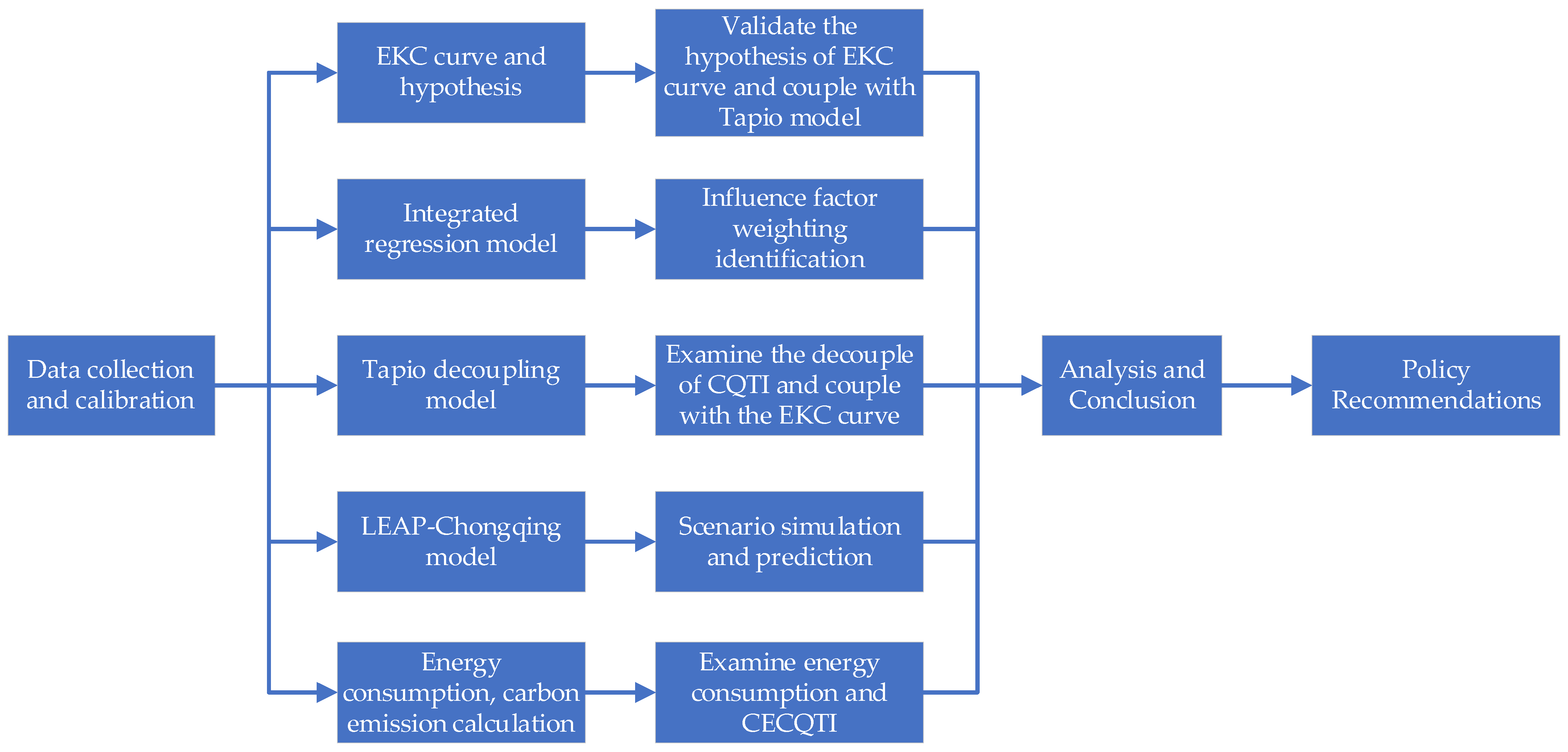
The research framework and route of this study are described in Figure 1.

2.1. EKC Curve and Hypothesis

Three kinds of tests are often mentioned in the study about the EKC curve model: linearity test, quadratic test, and cubic test. Grossman and Krueger first used the cubic test and found the N curve [23,24]. Some subsequent studies pointed out [25] that in the empirical process, the cubic test should be set first, and then the quadratic and linearity tests should be reduced one by one if the coefficients are not significant.

In this study, we make the following two hypotheses: (i) there is an inverse N-shaped relationship between the development of CQTI and environmental pressure from 2005 to 2020; (ii) there is an inverse N-shaped relationship between vehicle ownership and environmental pressure in Chongqing from 2005 to 2020. In other words, during the development of the transportation industry, the carbon emissions generated by the industry show a process of “decline–rise–decline”. This paper presents the two hypothetical EKC models as Equations (1) and (2), respectively:

$$LnC={\alpha }_0+{\alpha }_{1}LnGDP+{\alpha }_2{(LnGDP)}^2+{\alpha }_3{(LnGDP)}^3+\beta LnU+\epsilon$$

(1)

$$LnC={\lambda }_0+{\lambda }_{1}LnVEC+{\lambda }_2{(LnVEC)}^2+{\lambda }_3{(LnVEC)}^3+\mu LnU+\epsilon$$

(2)

In order to reduce the effect of the magnitude, all indicators are treated as logarithms. Where C denotes carbon emissions from the transportation industry, GDP denotes gross output value of the transportation industry, U denotes urbanization process, VEC denotes vehicle ownership, α_i (i = 0, 1, 2, 3), and λ_i (i = 0, 1, 2, 3) are parameters to be estimated, and ε is the random error term. Based on their coefficients, the EKC curves can be classified into the seven cases in

Table 1. EKC curve category.

Category	Coefficient Notation	The Relationship between Y and X
1	α1 = α2 = α3 = 0	No relation
2	α1 < 0, α2 = α3 = 0	Negative linear correlation
3	α1 > 0, α2 = α3 = 0	Positive linear correlation
4	α1 < 0, α2 > 0, α3 = 0	“U” shape
5	α1 > 0, α2 < 0, α3 = 0	Inverted “U” shape
6	α1 < 0, α2 > 0, α3 < 0	Inverted “N” type
7	α1 > 0, α2 < 0, α3 > 0	“N” shape

Note: ${\lambda }_i$ is of the same type.

.

2.2. Integrated Regression Model

The STIRPAT model was developed on the basis of the IPAT model. York [26] points out that the IPAT model does not allow for non-monotonic, differentially scaled changes in the influencing factors and is therefore extremely limited in its use; to overcome this shortcoming, the York STIRPAT model is put forward:

$$I=a{P}_i^b{A}_i^C{T}_i^d{e}_i$$

(3)

where a, b, c, and d are the parameters to be estimated by the model and e_i is the random error term. In practice, the above equation is generally estimated in a logarithmic form. In the STIRPAT model, the excellent topology allows P, A, and T to be decomposed into many factors that affect the environment [27,28]; therefore, this model has received more research attention [29,30,31]. The logarithmic form is given by Equation (4):

$$Ln{I}_i=Lna+bLn(P_i)+cLn(A_i)+dLn(T_i)+e_i$$

(4)

The outstanding advantage of the STIRPAT model is the enrichment of the influencing factors considered in this study. In order to further assess the weight of different influencing factors on CECQTI, we have adjusted and expanded the study indicators. In this study, car ownership is used as a proxy for traditional demographic factors, the Chongqing transportation output (CQTI-GDP) indicator is used to proxy the affluence brought by urban development, and the urbanization rate is used to proxy the technological progress of urban development. The improved integrated model is shown below:

$$Ln{C}_i=Lna+bLn(VE{C}_i)+cLn(GD{P}_i)+dLn(U_i)+e_i$$

(5)

where I denotes CECQTI, VEC denotes car ownership, GDP denotes CQTI-GDP, U denotes urbanization rate, e is the error term, and i (i = 2005, 2006, L, 2020) is the sample observation period. The a denotes the model constant term and b, c, d denote the coefficients of VEC, GDP and U, respectively.

2.3. Tapio Decoupling Model

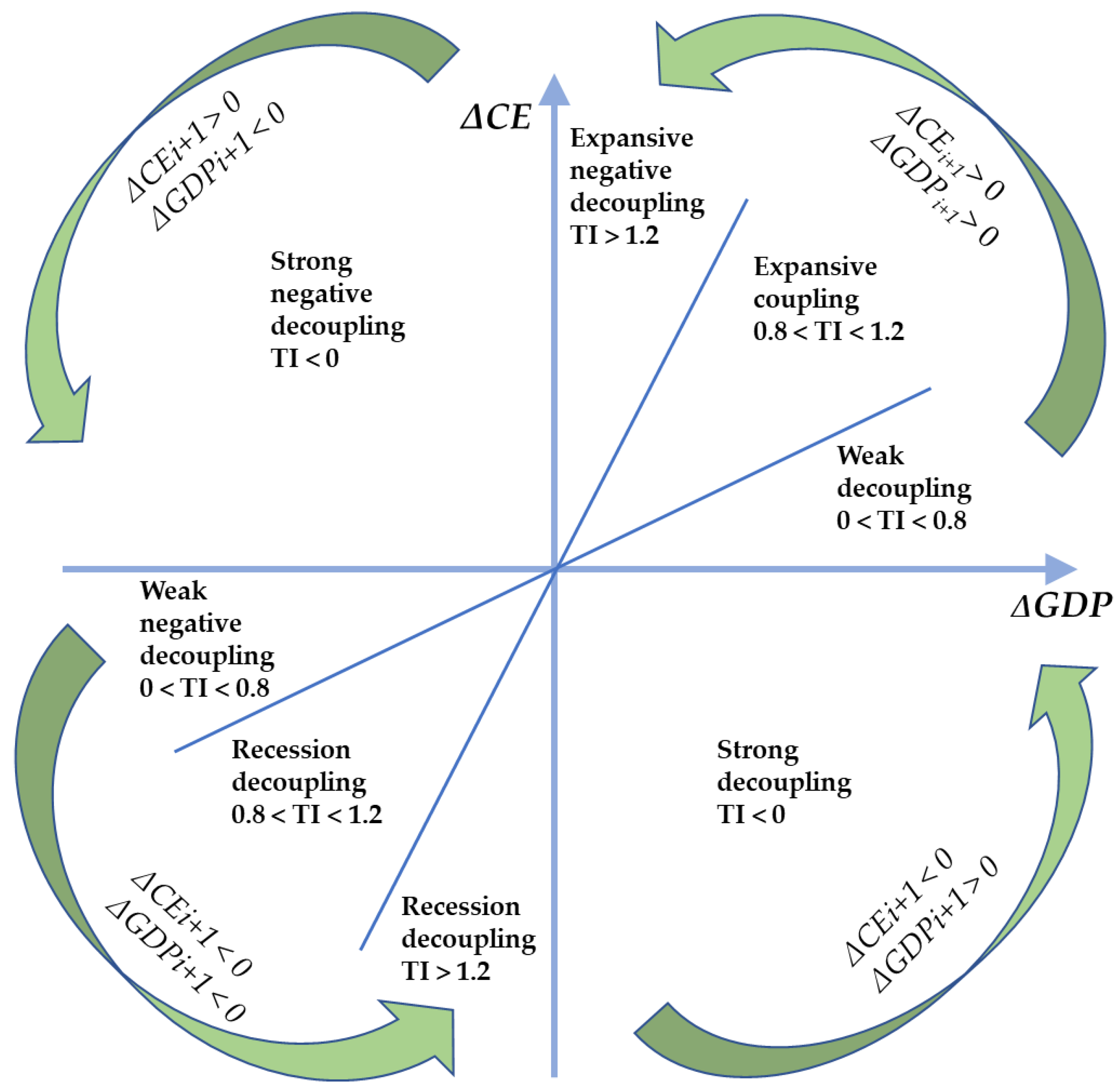
There is an inextricable link between economic growth and the ecological environment. The concept of decoupling was introduced as early as the 1960s, and decoupling implies the non-synchronous changes in the economy and resource environment. In 2005, Tapio [32] subdivided the decoupling relationship into eight states according to different decoupling elasticity indices, which is essential for constructing a scientific and complete decoupling index, and the Tapio decoupling model has been widely used by scholars in subsequent studies. The decoupling elasticity index is an indicator value that indicates the degree of change in environmental pressure due to the magnitude of change in economic development, and the decoupling elasticity index is calculated as follows:

$$T_{i+1}=\frac{\%\Delta C{E}_{i+1}}{\%\Delta GD{P}_{i+1}}=\frac{\Delta C{E}_{i+1}/C{E}_i}{\Delta GD{P}_{i+1}/GD{P}_i}$$

(6)

where T_i+1 denotes the decoupling elasticity index in period i+1, %ΔCE_i+1 and %ΔGDP_i+1 denote the growth rate of carbon emission and GDP in period i+1, ΔCE_i+1 and ΔGDP_i+1 denote the growth values of carbon emission and GDP in period i+1, and CE_i and GDP_i denote the values of carbon emission and GDP in period i, respectively. Eight different decoupling states are classified according to different T_i+1, ΔCE_i+1, and ΔGDP_i+1 values, as shown in Figure 2.

2.4. LEAP-Chongqing Model Building

The LEAP model is an integrated modeling tool for long-term scenario analysis developed by the Stockholm Environment Institute that can be used to track energy consumption and GHG emissions in all sectors. The LEAP model has excellent characteristics of low initial data requirements and long prediction time and has been applied in numerous countries and regions for residential living [33,34], industrial planning [35,36], and industry development (buildings [37], steel [38], electricity [39], transportation [11,18]) in the study of energy consumption and GHG emissions.

From 2005 to 2020, the average annual growth rate of vehicle ownership in Chongqing was as high as 14.99%, far exceeding the average GDP growth rate of the transportation industry, and the average annual growth rate of CECQTI was 6.80%. In order to examine the imbalance between environmental pressure and economic development and to evaluate the effectiveness of different carbon reduction measures, this study constructed the LEAP-Chongqing model by LEAP software. The LEAP-Chongqing model takes 2020 as the base year, contains one basic scenario and four forecast scenarios, and is based on relevant studies [11,18,40,41,42] and CQTI vision [21,22]. As shown in

Table 2. Settings for different scenarios.

Scenario Type	Scenario Description and Rationale
Base scenario (BAS)	Zero program scenario without any energy saving and emission reduction measures.
Transport modal shift scenario (TS)	Create an energy-saving and environmentally friendly green transportation system. Strengthen rail and waterway freight transport and reduce the proportion of road freight transport [21]. Passenger transport strengthens the proportion of public transport, especially rail transport, and the proportion of private transport is reduced accordingly [22].
Fuel shift scenarios (FS)	Invest in building a clean, low-carbon, and efficient energy system. Increase the share of clean energy and new energy vehicle ownership, and improve the use of compressed natural gas (CNG), liquefied natural gas (LNG), and electric energy in transportation fuels [22].
Energy efficiency scenario (ES)	Continuously improve energy efficiency and reduce the intensity of energy emissions, adhere to the priority of energy conservation, and strictly control energy consumption and CO2 emission intensity [22].
Integrated operating scenario (IO)	Based on BAS scenarios with the integration of TS, FS, and ES scenarios.

, it is important to note that to effectively quantify and compare the impacts of each scenario, this study assumes that the carbon emission factors for all energy sources remain constant at the base year level during the scenario simulation.

Qualitative descriptions of the above five scenarios are defined below, and detailed data on key parameters are presented in Supplementary Materials Tables S1–S5.

2.5. Data Source

The transportation industry has great potential to reduce emissions and is a hot research area for carbon emission reduction in recent years. Compared with other methods, the carbon emission factor method has the advantages of high efficiency and fast and accurate calculation [43,44]. Therefore, the carbon emission factor method is chosen to calculate the carbon emissions of the transportation industry in this study. The calculation formula is as follows:

$$\begin{array}{c}C={\displaystyle \sum E_i\times F_i}\\ \hspace{1em}\hspace{1em} ={\displaystyle \sum e_i}\times k_i\times F_i\end{array}$$

(7)

In Formula (7), C indicates the total carbon emission of the transportation industry (million tons); E_i indicates the standard coal consumption of energy type i (million tons), F_i indicates the carbon emission coefficient of energy type i; e_i is the consumption of various types of energy before converting standard coal; ki indicates the converted standard coal coefficient of various types of energy.

$$CI=\frac{C}{GDP}$$

(8)

$$EI=\frac{E}{GDP}$$

(9)

In Equations (8) and (9), C and E represent the CO₂ emissions and total energy consumed by the transportation industry, respectively, and GDP is the gross transportation product.

The data sources for this study are as follows: GDP-CQTI from Chongqing Statistical Yearbook (2006–2021) [45], car ownership from China Transport Statistical Yearbook (2006–2021) [46], energy consumption and standard coal coefficient from China Energy Statistical Yearbook (2006–2021) [47], and carbon emission coefficient from the Guide to Provincial Greenhouse Gas Inventories [48].

3. Results

3.1. Analysis of CECQTI Calculation Results

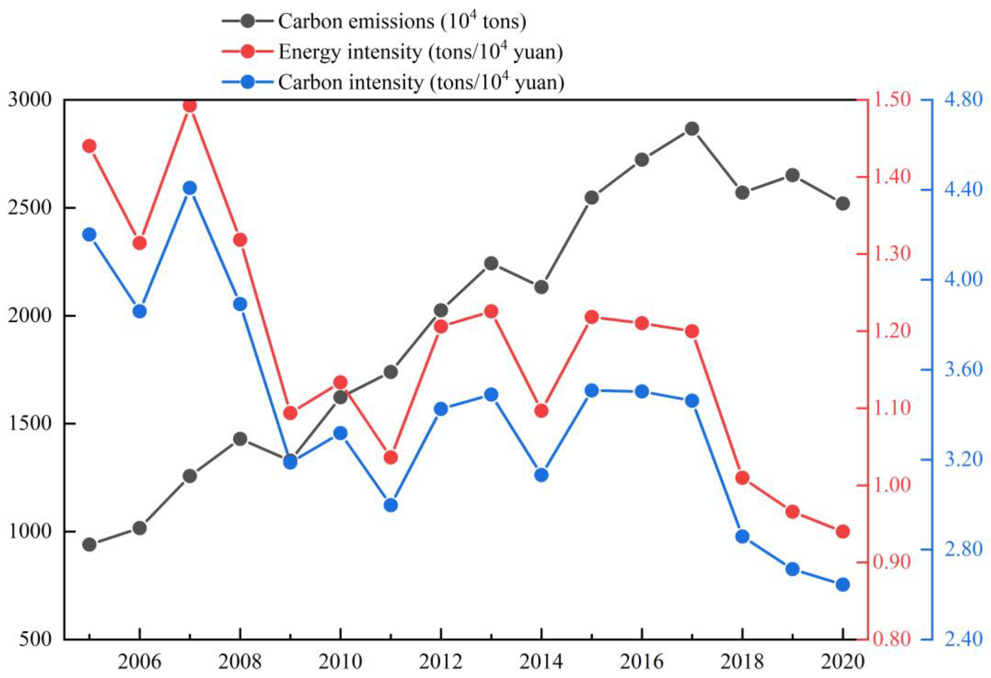
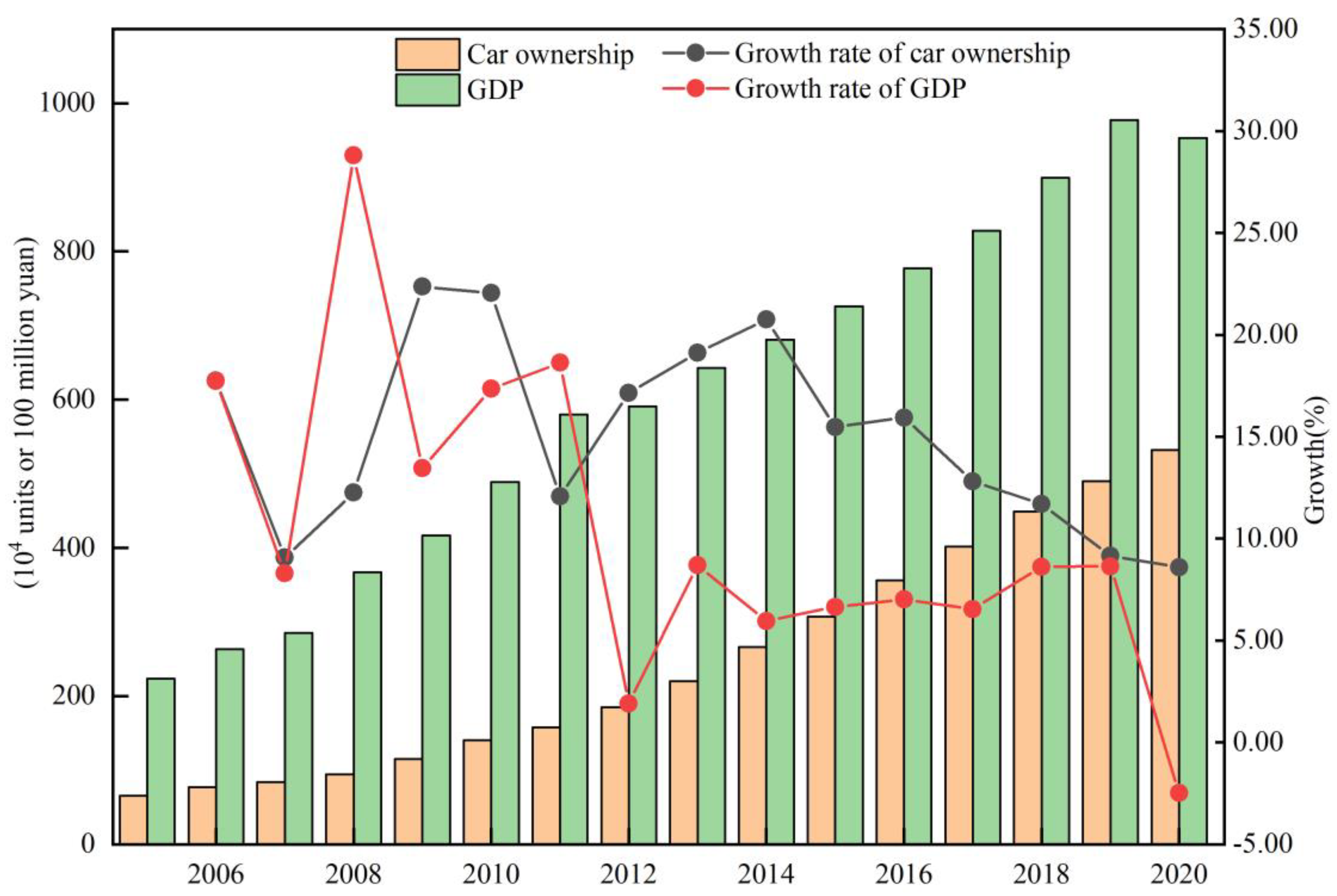
The calculation results are shown in Figure 3 and Figure 4 for CECQTI, CI, EI, car ownership growth rate, and carbon emission growth rate, respectively. From the figure, it can be seen that CECQTI shows a phased growth trend in scale effect, with significant growth trends from 2005–2008, 2009–2013, and 2014–2017, and a certain moderating trend from 2008–2009 and 2013–2014, and carbon emissions grew from 9.395 Mt in 2005 to 25.195 Mt in 2020, with a growth rate of 168.17%. During the calculation period, after CECQTI reached a short-term peak of 28.666 Mt in 2017, it shows a decreasing trend, and the rate of decrease reaches 12.11% by 2020. EI and CI play an essential role in measuring the total carbon emissions, and the total carbon emissions can be significantly reduced when EI and CI decrease significantly at the same time. Combined with Figure 3, we can see that the trend of CI and EI curves are very similar, both peaking in 2007, followed by phase fluctuations, and gradually showing a decreasing trend since 2015. CECQTI then has the highest value in the calculation period in 2017, after which carbon emissions show a decreasing trend. It should be noted that 2017 is not necessarily the carbon peaking year of CQTI, and relevant studies [49] and international experience [50] show that in order to avoid false peaking effectively, if the amount of data (number of years) of the urban emission time series after the maximum year in the calculation period are less than five years, the carbon emission of the region is considered not peaking, and greater than five years may be located in the plateau period, and further trend testing is required. Therefore, the carbon emissions of CQTI started to enter the plateau period in 2017.

In 2021, Beijing, Chengdu, and Chongqing were three cities with more than five million cars. Chongqing ranks third with 5.636 million units. As can be seen from Figure 4, Chongqing’s car ownership grew from 654,100 units in 2005 to 5,321,600 units in 2020, with a growth rate of 713.37% and an average annual growth rate of 14.99%. The growth rate of Chongqing’s car ownership between 2005 and 2018 remained above 10% except for a few years, and the growth rate from 2018 to 2020 slowed down and stayed at about 8%. The highest growth rate occurred in 2008–2010, above 22%, showing that the number of cars purchased in Chongqing showed rapid growth during these two years. The 2013–2014 growth rate peaked at 2.66 million cars, after which the growth rate of ownership steadily declined. CNY 95.287 billion, a growth rate of 326.09%, with an average annual growth rate of 110.15%, occurred. The highest growth rate of CQTI-GDP appeared in 2008, reaching 28.81%, then dropped to below 20%, and the whole of 2013–2019 showed a more stable state, remaining at about 8%. Suddenly, 2019–2020 shows a sharp decline, from 8.65% to −2.5%, with fluctuations of up to 10%.

In summary, the CECQTI entered a plateau in 2017, with a peak of 28.666 Mt during the calculation period. The CI and EI have shown a decreasing trend since 2015, which has positively contributed to the reduction of the CECQTI. Vehicle ownership in Chongqing shows a quick growth trend, but the GDP of the transportation industry shows negative growth. These pieces of evidence indicate that CQTI has a strong potential for low-carbon and carbon reduction.

3.2. ECK Curve Fitting

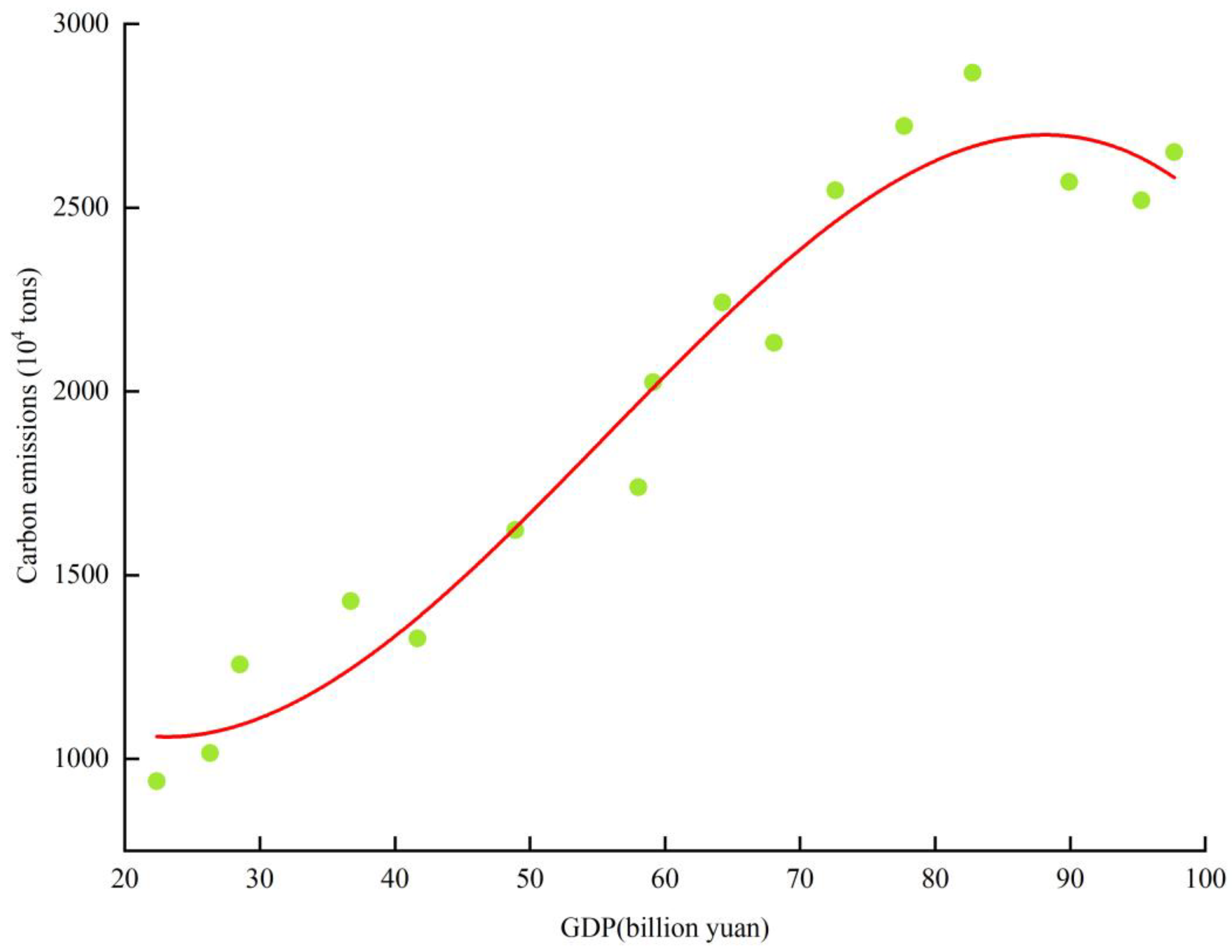
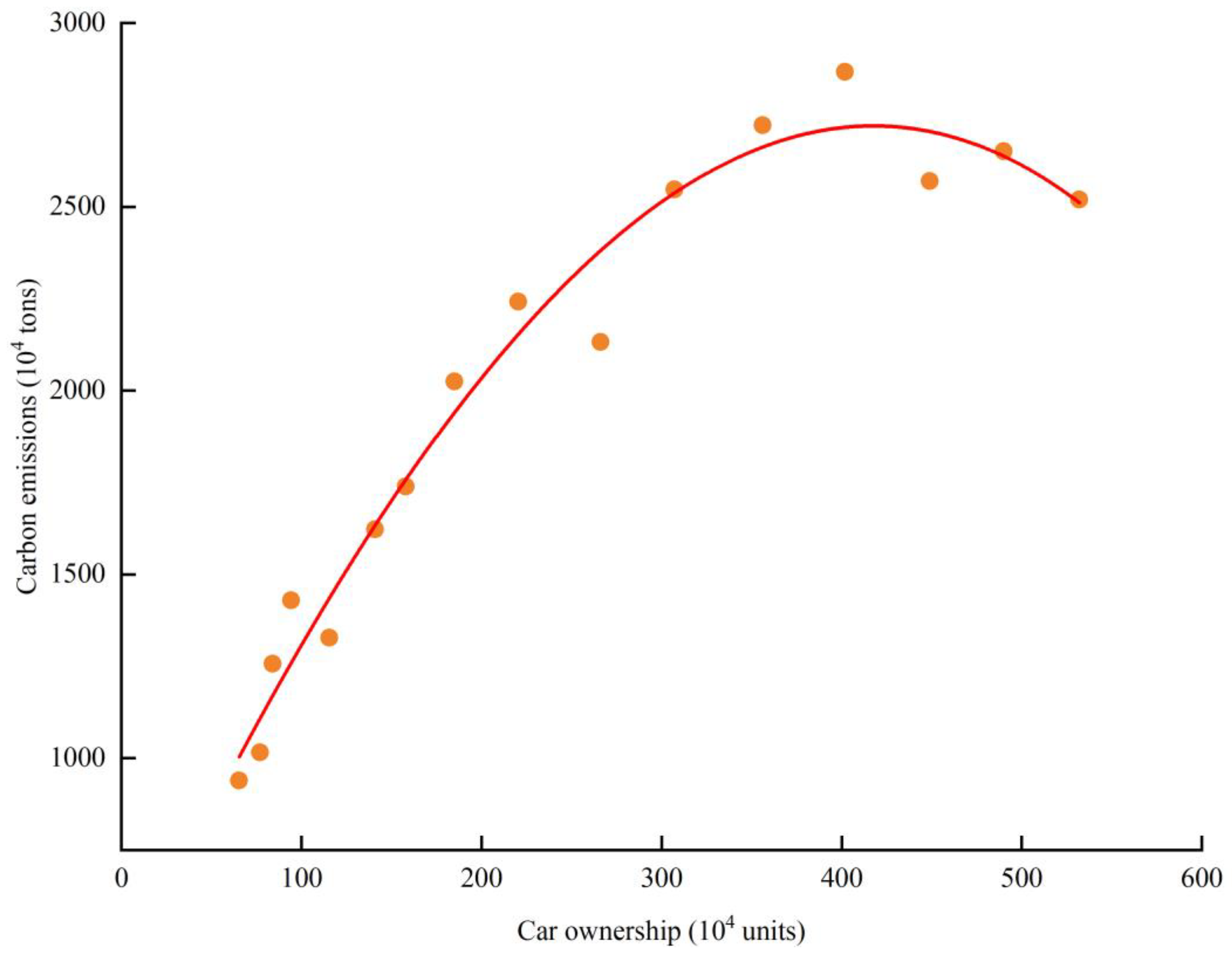
After the calculation of CECQTI in the previous section, this section fits CECQTI to CQTI-GDP and Chongqing city car ownership, respectively, as shown in Figure 5 and Figure 6. Among them, the fitting of carbon emissions and GDP shows a certain inverted N-shaped trend, and the fitting of carbon emissions and car ownership shows a certain inverted U-shaped trend. However, this does not mean such a trend is inevitable between carbon emissions and GDP and car ownership, and it needs to be verified afterwards. In the process of economic and environmental development, it is greatly influenced by the urbanization process [51], so this study introduces the urbanization rate as a control variable in the EKC curve model.

In order to effectively prevent pseudo-regression of time series data, the time series data were tested for smoothness using the ADF unit root test and further Granger causality test. The results of the ADF unit root test are shown in

Table 3. ADF unit root test results.

Variable	Type of Inspection	ADF Test	Confidence Interval Level			p Value
	(c, t, q)	Statistic	1%	5%	10%
LnC	(c, t, 2)	−4.423 **	−5.296	−4.008	−3.461	0.030
LnGDP	(c, t, 2)	−4.437 **	−4.992	−3.875	−3.388	0.022
LnVEC	(c, t, 2)	−6.506 ***	−5.125	−3.933	−3.420	0.002
LnU	(c, t, 2)	−5.055 ***	−4.886	−3.829	−3.863	0.008

Note: ** and *** indicate significance at the 10%, 5%, and 1% levels, respectively; (c, t, q), in which c, t, and q represent the constant term, the time trend, and the lag, respectively.

. The unit root tests in log form for carbon emissions, transportation output, car ownership, and urbanization are significant at the 5%, 5%, 1%, and 1% levels, respectively. Therefore, we believe that these variables pass this test step and can proceed to the next step of the Granger causality test analysis. The Granger causality test is shown in

Table 4. Granger causality test results.

Null Hypothesis	F-Statistic	p Value
LnGDP does not Granger Cause LnC	3.630 *	0.070
LnC does not Granger Cause LnGDP	0.325	0.731
LnVEC does not Granger Cause LnC	5.631 *	0.094
LnC does not Granger Cause LnVEC	0.895	0.559

Note: * indicate significance at the 10%, 5%, and 1% levels, respectively.

, which shows that “LnGDP does not Granger Cause LnC”, which rejects the original hypothesis at the 10% level. The null hypothesis that “LnC does not Granger Cause LnGDP” is not rejected, and the statistical test indicates that GDP is the cause of the growth of carbon emissions. Similarly, it is clear from the results of the Granger causality test that car ownership is also responsible for the growth of carbon emissions.

This study examined two models to examine the EKC curve relationship between CQTI-GDP and car ownership with carbon emissions. The results are shown in

Table 5. EKC curve fitting results.

Variable	Model 1	Model 2
C	25.288 ** (12.088)	120.121 * (61.314)
LnGDP	−25.541 ** (10.730)
(LnGDP)2	4.930 ** (1.963)
(LnGDP)3	−0.324 ** (0.124)
LnVEC		−66.602 * (30.664)
(LnVEC)2		11.304 ** (5.007)
(LnVEC)3		−0.641 ** (0.273)
LnU	6.800 ** (2.977)	4.651 ** (1.720)
Adjust R2	0.978	0.970
F	124.804	89.780
P	0.000	0.000
DW	2.154	2.268

Note: * and ** indicate significance at the 10%, 5%, and 1% levels, respectively.

. The primary, quadratic and cubic terms of CQTI-GDP are significant at the 5% level, and α1 < 0, α2 > 0, and α3 < 0. This indicates an inverted N-shaped curve between CQTI-GDP and CECQTI, which verifies the previous hypothesis of this study.

Similarly, this paper examines the EKC curve relationship between car ownership and environmental stress in Chongqing city. The results show that the primary, quadratic and cubic terms of car ownership in Chongqing are significant at 10%, 5%, and 5% levels, respectively, and λ1 < 0, λ2 > 0, λ3 < 0. This indicates an inverted N-shaped curve between car ownership and CECQTI in Chongqing, which is also consistent with the previous hypothesis of this paper. Although Figure 6 shows an inverted U-shape to some extent, the conclusion is more inclined to the calculated results.

In the validation of both models, it can be seen that the control variable urbanization rate is significant at the 5% level. The finding that the effect of the urbanization rate on carbon emissions shows a positive contribution is in line with common sense. The development of urbanization will bring pollution to the environment to a certain extent and cause an increase in carbon emissions. As a side reaction, a higher urbanization rate is not better, and in some cities with a high urbanization rate, the urbanization rate does not represent the economic development level of the city. However, it may be accompanied by more “agricultural to urban” residents [31]. It is more important to reconcile the relationship between economic development and environmental pollution.

In summary, the relationship between CQTI-GDP and car ownership and CECQTI shows an inverted N-shaped relationship, and the peaks of both models have appeared in the short term and are now in the declining stage. With the continuous development of the industrial economy, transportation carbon emissions show an “improvement-deterioration-improvement” stage of development. This indicates that in the foreseeable long term, with the continuous development of CQTI, CECQTI shows a significant downward trend, and the trend is gradually improving.

3.3. Integrated Model Impact Weight Analysis

Equation (5) discusses the weights of each influencing factor using PLS. PLS is suitable for small sample sizes and data with multicollinearity [52]. The difference between PLS and ordinary least squares is that it can filter and extract the factors in the model that have the greatest influence on the dependent variable, identify the valid information in the regression process, and match the best function, which allows PLS to obtain more reliable regression results [53,54].

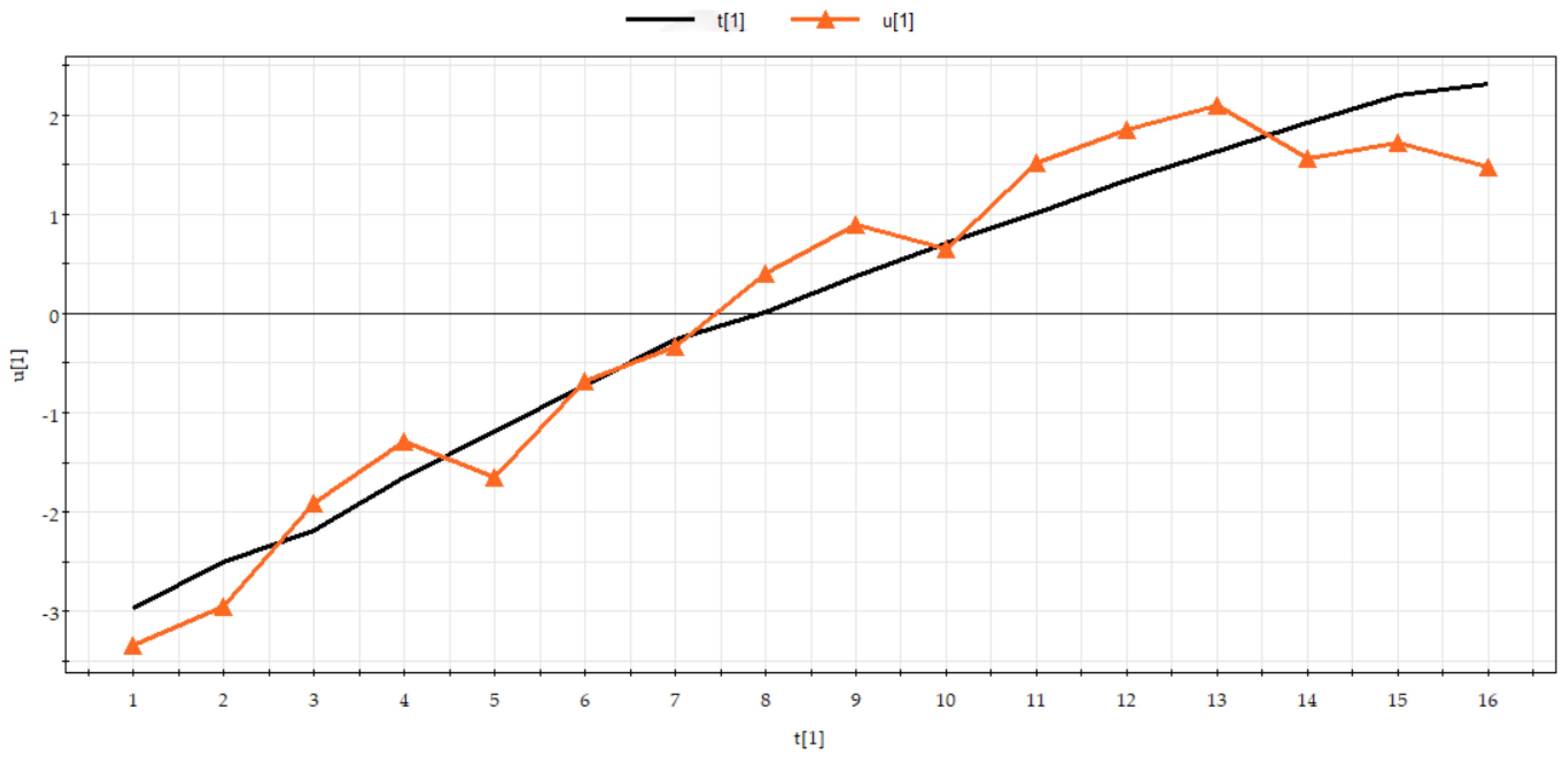
Firstly, two kinds of t1/u1 scatter plots, and T² ellipse plot are used to judge the degree of goodness of PLS fit. The software extracts the principal components with typical characteristics in PLS regression, and the linearity is judged by t1/u1 scatter plot and T2 ellipse plot to determine whether the linear relationship is good, and then the weight of the influence of the independent variable on the dependent variable [55].

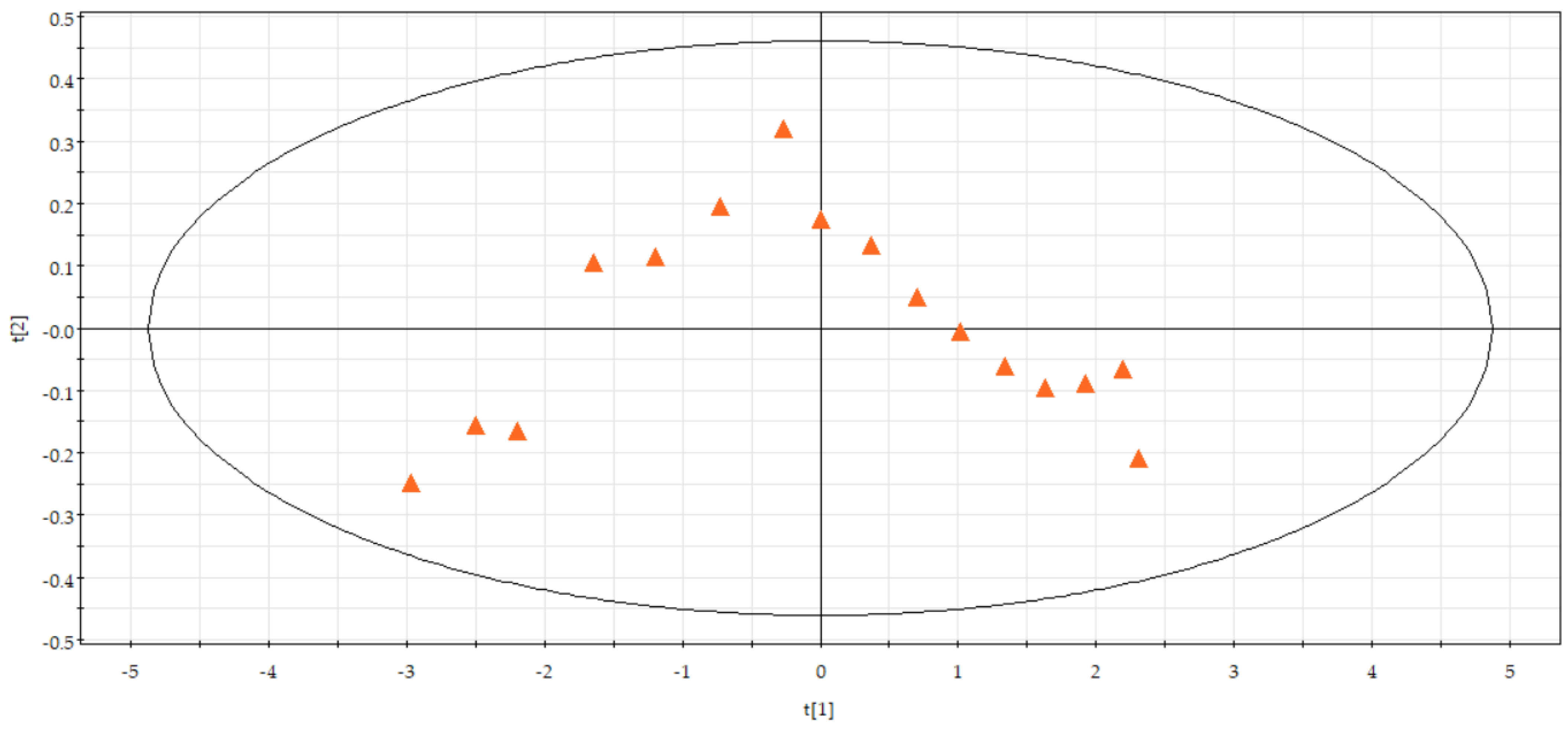
In the t1/u1 scatter plot, u1 is the first principal component of Y after extracting one principal component t1. It is shown that the closer the correlation between the extracted principal component t1 and u1 is to linearity, the more reasonable the PLS regression is. As can be seen, in Figure 7, the points in the plot show a good linear relationship with R² = 0.991, which indicates that the integrated regression model with PLS is reasonable. The idiosyncratic points where the observed values are far from the average can be found by observing the distribution characteristics of the sample points of the T² ellipsoidal plot on the plane t1/u1 scatter plot in the high-dimensional space. It can be seen from Figure 8 that although some of the sample points are some distance away from the center, they are all inside the ellipse, so the sample points in the model are taken as reasonable values.

The SIMCA software automatically fits the sample data to generate R2Y (cumulative explanatory power) and Q2 (cross validity). These indicators are, to some extent, explanatory for the soundness of the model. As can be seen from

Table 6. Integrated regression model PLS information.

Model	N	R2X	R2Y	Limit	Q2 (cum)
Comp 1	2	0.999	0.945	0.05	0.927

, the software extracted two components from the set of independent variables, and they generalized the set of independent variables with 92.7% accuracy, and the equation explained the CECQTI with 94.5% accuracy. The R2X, R2Y, and Q2 (cum) values in the table are more significant than 0.9, and the regression results are usually considered ideal [52].

The influence weight of each variable in the integrated regression model was measured by the variable projection importance analysis (VIP) response, using the calculated VIP value, with a higher VIP value indicating a higher influence weight of the variable. The importance of the VIP values is shown in

Table 7. Analysis of integrated regression model results.

Variable	VIP Value	Coefficient
LnGDP	1.012	0.769
LnU	0.995	0.111
LnVEC	0.993	0.096
R2	0.991	0.999

as follows: total transportation output value (1.012) > urbanization rate (0.995) > car ownership (0.993), R2 = 0.991. The VIP values show that the increase in total transportation output value is the most important factor for the increase in carbon emissions in the transportation industry. At the same time, the urbanization rate and car ownership have less influence on the increase in carbon emissions in the transportation industry. The influence of urbanization rate and vehicle ownership on the increase in carbon emissions in the transportation sector have a slightly smaller weight, but both are close to 1, indicating that they both have a significant influence. The regression coefficients of the equation show that 1% of GDP, urbanization rate, or car ownership will cause 0.769%, 0.111%, and 0.096% changes in carbon emissions, respectively, with other variables held constant.

3.4. Tapio Decoupling Analysis

The decoupling status of CQTI is shown in

Table 8. Chongqing transportation and environmental stress decoupling information.

The Annual Phase	ΔCEi+1	ΔGDPi+1	Ti+1	Decoupling State	State Description
2005–2006	0.082	0.177	0.460	Weak decoupling	Good
2006–2007	0.237	0.083	2.855	Expansive negative decoupling	Poor
2007–2008	0.137	0.288	0.476	Weak decoupling	Good
2008–2009	−0.071	0.135	−0.527	Strong decoupling	Best
2009–2010	0.222	0.174	1.277	Expansive negative decoupling	Poor
2010–2011	0.072	0.186	0.385	Weak decoupling	Good
2011–2012	0.165	0.019	8.672	Expansive negative decoupling	Poor
2012–2013	0.107	0.087	1.234	Expansive negative decoupling	Poor
2013–2014	−0.049	0.060	−0.825	Strong decoupling	Best
2014–2015	0.194	0.066	2.927	Expansive negative decoupling	Poor
2015–2016	0.069	0.070	0.981	Expansive coupling	Average
2016–2017	0.053	0.065	0.810	Expansive coupling	Average
2017–2018	−0.103	0.086	−1.198	Strong decoupling	Best
2018–2019	0.031	0.086	0.363	Weak decoupling	Good
2019–2020	−0.050	−0.025	1.999	Recession decoupling	Better

. We can clearly see that the CECQTI shows a fluctuating cross-change trend and basically maintains the form of “development-pollution-development”, which is consistent with the hypothesis that the relationship between CECQTI and CQTI-GDP shows an inverted N-shaped curve.

During 2005–2020, the decoupling status is above “Average” for 11 years, indicating an overall positive trend in the decoupling status of CQTI. However, in some years, the “expansionary negative decoupling” status is maintained for a long time.

The expansionary negative decoupling represents slow economic growth and a rapid increase in pollution. Combined with Section 3.1 and Table 8, it can be seen that the years with negative expansionary decoupling have lower GDP growth and stronger carbon emission growth rates. It is found that in these years, the growth rate of Chongqing’s car ownership reached the highest 22.05% and jumped to the top three in the country in 2014, which puts great pressure on the decoupling of CQTI. At the same time, the rapid development of CQTI in these years, the rapid increase in turnover, and the unreasonable energy structure can also explain, to some extent, the expansive negative decoupling state seen in these years.

The strong decoupling state is the best state of development, representing a stable economic growth and a gradual decrease in pollution. There are three strong decoupling states in the calculation period, in 2008–2009, 2013–2014 and 2017–2018. Surprisingly, the strong decoupling states tend to appear after the aforementioned expansionary negative decoupling states, suggesting that the increase in environmental pollution is often accompanied by environmental protection policies. For example, in 2008, the “Key Points of Energy Conservation and Emission Reduction in the National Transportation Industry” proposed to increase capacity restructuring and strengthen technological innovation in energy conservation and emission reduction. In 2011, the “12th Five-Year Plan for Energy Conservation and Emission Reduction in Transportation” proposed to build an environmentally friendly transportation industry by improving energy efficiency and reducing carbon emission intensity. These policy philosophies directly influence the direction of energy conservation levels, and also to some extent explain the strong decoupling that occurred during the above years. Likewise, the data survey also shows that the growth rate of car ownership in Chongqing was slow, at around 10%, during the above decoupling period, and that these phases should be located in the downward phase of the inverted “N” shape over the peak point.

Weak decoupling, recessionary decoupling, and expansionary coupling are the more common and optimistic states, and the longest period covered is 2015–2020, an important period in China’s 13th Five-Year Plan. The 13th Five-Year Plan outlines a number of binding targets and expected hard targets for China’s ecological protection. Economic development is guaranteed in these three states, and environmental pollution is different. Generally speaking, economic development’s growth rate is higher than environmental pollution’s rate. Observing the coupled states in the calculation period, it can be seen that the above three coupled states tend to be more coherent in time span and have certain long-term timeliness. China became the world’s largest carbon emitter in 2007 [56], and with the implementation of the Kyoto Protocol, the issue of carbon emission reduction in various industries has attracted the attention of many scholars and also become an important task for China. The signing of the Paris Agreement in 2016 also put forward higher requirements for carbon emission reduction in China. The above three coupled states often appear within one or two years after the promulgation of various energy conservation requirements, which indicates that both China’s internal energy conservation policies and international energy conservation policies have played a role in carbon emission reduction, albeit with certain characteristics, such as a certain lag or poor continuity in certain periods.

In summary, the impact of implementing energy conservation and emission reduction policies on decoupling is huge, both in China and Chongqing, China. In Chongqing, the overall decoupling status is in the form of “governance-pollution-governance”, and the environmental status is also in the trend of “good-poor-good”. At the same time, the trend between car ownership and environmental pressure is inverted N-shaped. At present, the overall development of CQTI is showing a positive trend, but it will still face many challenges. To effectively deal with these challenges, it is necessary to construct a new idea of phased constraint targets, strengthen the research on emission mechanisms and influencing factors, and formulate dynamic, practical, and localized emission reduction plans for the transportation industry.

3.5. EKC Curve and Tapio Coupling Integration Analysis

The EKC curve generally describes the long-term relationship between economic development and regional environmental stress, while the Tapio decoupling model focuses more on short-term characteristics. From a sustainability and assessment perspective, the decoupling index may be linked to different stages of the inverted U- or inverted N-curve in the course of sustained economic growth, as shown in Figure 9.

The EKC curve and Tapio decoupling model are coupled and integrated in Figure 9 into four regions, A, B, C and D [57]. TI = 1.2, TI = 0.8 and TI = 0 are the turning points of strong decoupling and coupling, respectively. Stage A indicates expansionary negative decoupling, where economic development comes at the cost of environmental stress. Stage B is slightly better than stage A, where economic development is synchronized with environmental stress. Stage D is the best, where rapid economic growth is accompanied by rapid environmental decline.

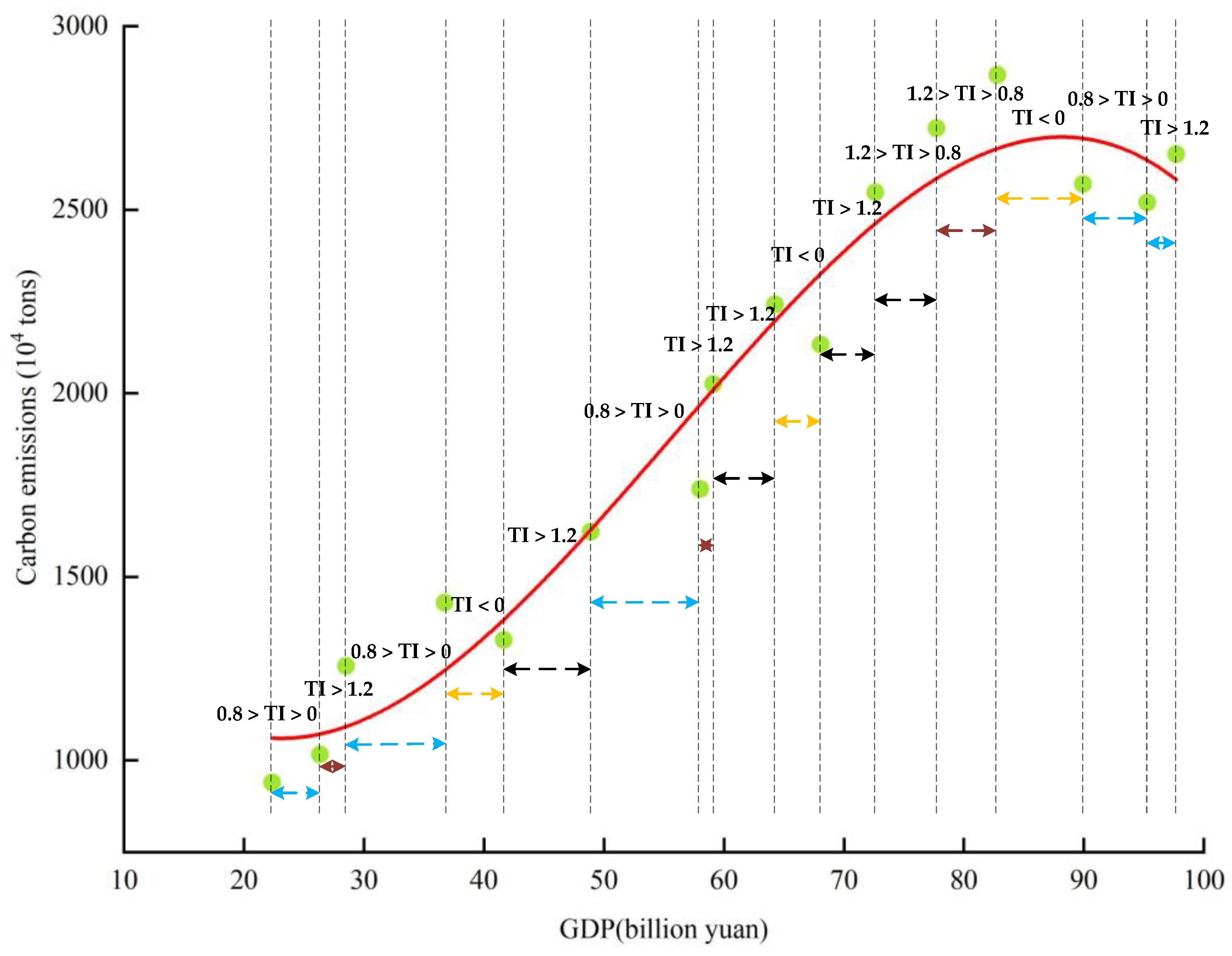
Combining the EKC curves of CQTI with the Tapio decoupling model, as shown in Figure 10, we can find that both TI = 1.2 and TI = 0 alternate, while TI = 0.8 does not appear in the calculation period, and as mentioned before, the difference between region B and region C is not obvious and often combined in the analysis [58]. Different coupling states alternate during the development of CQTI, but there are still patterns in them. A horizontal axis intercepts smaller than the vertical axis intercept and is often accompanied by a not-so-good coupling state, such as expansive negative decoupling. While the horizontal axis intercept is larger than the vertical axis intercept, it is usually a stage with a better development state, such as weak decoupling and declining decoupling. It is also found that the intercept of the trend point in the latter year of the graph is lower than that of the previous year, which is usually a year with the best state of economic development and environmental pressure, indicating that it may be a year of environmental pollution control, leading to a rapid recovery of control after serious pollution. After crossing the peak point, the development of CQTI as a whole shows a positive trend, and the development of economic development and environmental pressure is stable. However, in the current situation, the overall development of CQTI is still facing the double pressure of economic development and environmental protection.

In summary, the development of CQTI has been costly in terms of environmental pollution over a long period of time, although it occasionally shows a better decoupling during the calculation period, as mentioned in Section 3.4, often after the enactment of energy conservation and environmental protection policies. This suggests that in the early stages of rapid economic development or recovery, Chongqing and the world at large typically adopted a “pollute first, treat later” development model to deal with the current development crisis. Chongqing and even China’s transportation industry should focus on new technologies, new techniques, and new standards of change and establish a mechanism of energy reversal in line with China’s national conditions while focusing on the introduction of industry technology to explore a broader path for future research.

3.6. LEAP-Chongqing Scenario Analysis

3.6.1. Energy Consumption Analysis

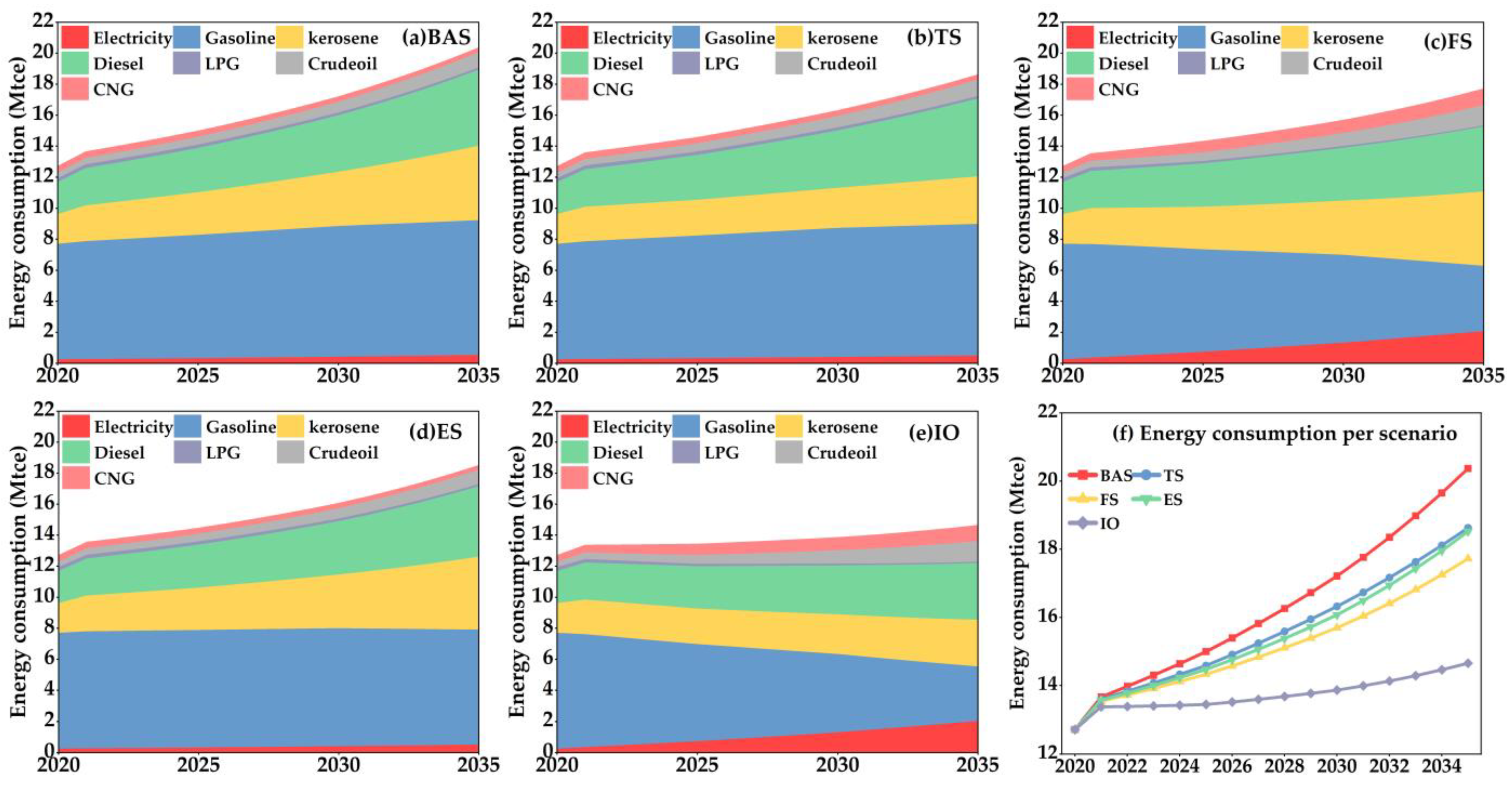
The energy consumption of the five scenario models, when converted to standard coal, is shown in Figure 11. The annual baseline consumption is 12.72 Mtce.

In terms of total energy consumption, the five scenarios have the highest to lowest energy consumption growth from 2020–2035: BAS, TS, ES, FS, and IO, with the BAS scenario reaching 20.37 Mtce in 2035, with a growth rate of 60.10% during the calculation period. The energy consumption growth rate in the IO scenario is the slowest, with an average annual growth rate of less than 1% and the lowest growth rate of 15% between 2020 and 2035. In addition, the energy reduction rates of the TS, FS, ES, and IO scenarios relative to the BAS scenario in 2035 are 8.55%, 12.98%, 9.07%, and 28.04%, respectively.

Looking at the energy consumption structure, in all five scenarios, gasoline, diesel, and aviation kerosene occupy the top three consumptions, and the total share of the three is as high as 80–90%. Electricity and CNG are the bottom two consumptions, and the total share of the two is as low as 5–13%. The energy structure of BAS, TS and ES scenarios does not change much. The energy structure tends to improve in FS and IO scenarios, and gasoline consumption decreases yearly. The gasoline consumption in 15 years decreased by 43.47% and 53.10% in the FS and IO scenarios, respectively, and the share of electric energy consumption increased year by year, from 2% to 14% over 15 years.

Each scenario has a certain inhibitory effect on energy consumption growth compared with the BAS scenario, but the optimization of energy structure is only well reflected in the FS and IO scenarios. Therefore, the future development of CQTI, FS, and IO scenarios can achieve energy diversification and promote the development of clean energy, which is expected to achieve environmentally friendly development.

3.6.2. Carbon Emission Analysis

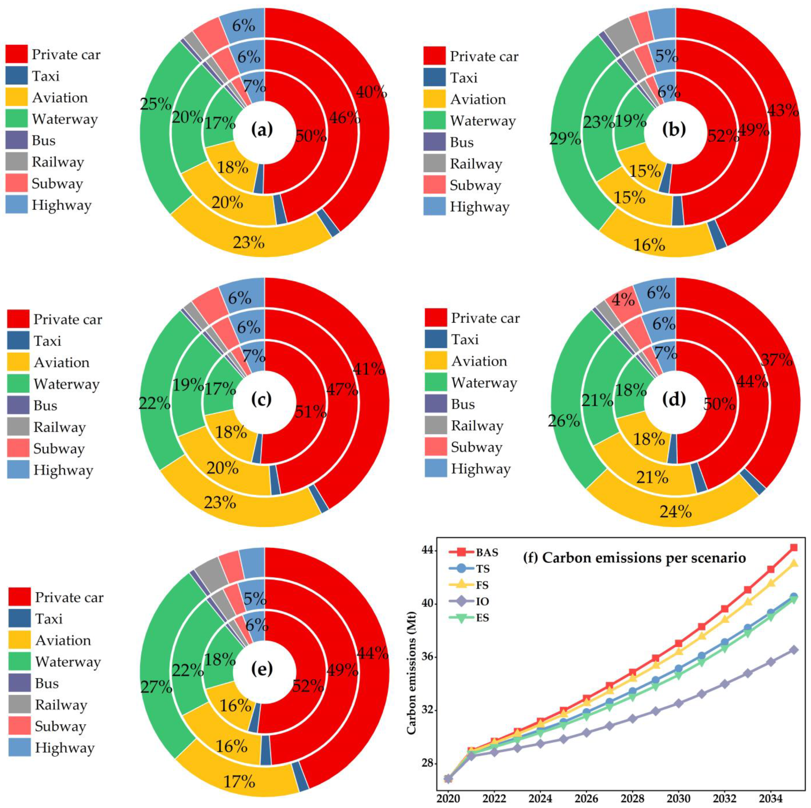
The carbon emission scenarios for the five scenario models are shown in Figure 12. The circles indicate 2025, 2030, and 2035, from inside to outside. The baseline annual carbon emissions are 26.90 Mt.

In terms of total carbon emissions, from 2020 to 2035, compared with the BAS scenario, the carbon emissions of the other four scenarios have decreased, and the carbon emission reductions are FS, TS, ES, and IO in descending order. The carbon emissions of the BAS scenario are 26.90 Mtce in 2020 and 44.25 Mtce in 2035, with a growth rate of 64.50% and an average annual growth rate of 3.37%. The IO scenario 2035 carbon emissions are 36.57 Mtce, with a growth rate of only 35.95%, which is the lowest among all scenarios.

Looking at the sources of carbon emission generation, through Figure 12, it can be found that from 2025 to 2035, regardless of that scenario, the carbon emissions generated by private cars are the highest, accounting for about 41–52%, and the proportion of carbon emissions from private cars is gradually decreasing with the growth of time and changes in energy structure and transportation modes. In the TS scenario, with the change of transportation mode, the private car trips are changed to public transportation trips, and the road transportation is changed to railroad and waterway transportation modes. The FS scenario implements fuel substitution measures and develops clean fuel vehicle technologies to reduce dependence on fossil energy. Among these scenarios, the FS reduces the carbon emissions of high-carbon emission transportation modes. However, the overall carbon reduction effect is not particularly good, which indicates that it is difficult to effectively reduce the total carbon emissions by improving the technology level alone in the development of the economy and the increasing transportation volume. The ES scenario model has improved energy efficiency in the transportation sector, and the carbon emission reduction of high-carbon emission transportation modes is large. This scenario has better carbon emission reduction performance, which indicates that energy efficiency improvement is an important part of carbon emission reduction in the future. The IO scenario is the most efficient scenario model for carbon emission reduction among all scenarios. In the IO scenario, we enhance the growth rate of car ownership compared to the other four scenarios. In this model, private cars are the largest source of carbon emissions, followed by water and air transportation, and the carbon emissions of other modes do not change much. Although the share of carbon emissions from water and air transportation is increasing, the IO scenario is still the most efficient scenario for carbon reduction. This indicates that even with rapid economic development and increasing car ownership, the total carbon emissions can be reduced without affecting the state of economic development if effective measures can be adopted.

In summary, private cars account for 41–52% of carbon emissions and are the key to carbon emission reduction in CQTI. In addition, the carbon emissions of FS, ES, TS, and IO scenarios decreased by 2.76%, 8.74%, 8.30%, and 17.36%, respectively, compared with the BAS scenario. This indicates that different emission reduction measures can reduce carbon emissions, but different measures have different characteristics, if only one of these strategies is implemented alone, the energy saving and emission reduction effect is not satisfactory. Therefore, the pooling of these measures mentioned above should be considered in subsequent policy studies, which is of great significance for CECQTI.

4. Conclusions and Discussion

This study analyzes and discusses the CECQTI, CI, EI, car ownership, and carbon emission growth rate. The EKC curve of CQTI is validated, PLS effectively analyzes the integrated regression model, and then the development of CQTI is explored by coupling and integrating Tapio decoupling analysis and EKC curve. Finally, the LEAP-Chongqing model was used to construct five scenarios to predict and analyze the energy consumption and carbon emissions of CQTI.

• The study results show that CECQTI reached a plateau in 2017, with a peak carbon emission of 28.66 MtCO₂ during the calculation period. EI and CI also play an important role in reducing carbon emissions, showing a decreasing trend from 2015 onwards. The growth rate of car ownership in Chongqing is higher than 8%, which puts more pressure on the carbon emission reduction of CECQTI.
• The EKC curves between CQTI environmental pressure, car ownership, and transportation industry output show inverted N-shaped curves. The development of the transportation industry is usually accompanied by a “pollution-cure-pollution” or “development-decline development” pattern, and economic growth causes environmental pressure and also forces environmental improvement [59]. Reducing carbon emissions generated by the transportation sector is a requirement of China’s sustainable development strategy, and establishing a low-carbon and efficient transportation system is a good choice for Chongqing, a Chinese mountain city.
• The PLS integrated regression model shows that among the factors affecting the growth of CECQTI, 1% of GDP, urbanization rate, or car ownership will cause 0.769%, 0.111%, and 0.096% changes in carbon emissions, respectively. Car ownership is not an uncontrollable factor that brings environmental pollution, and promoting low-energy, low-pollution cars is an important way to reduce carbon emissions effectively [18,19].
• In the integrated analysis of the EKC curve and Tapio model of CQTI, the decoupling state shows an interval distribution, and the impact of energy saving policy has a certain lag. Furthermore, this indicates that the development of the transportation industry has long been at the cost of environmental pollution and even deteriorated [60], but this state has moderated and tended to be better since 2017. Related research shows [61] that CQTI gradually entered a low growth period from 2016, which is conducive to CQTI industrial restructuring. China’s economic development is increasingly dependent on the transportation industry, and the development of CQTI can reduce the carbon emissions generated by CQTI by adjusting transportation modes to improve the efficiency of transportation operations.
• According to the LEAP-Chongqing model, it is known that by 2035, the energy consumption of TS, FS, ES, and IO scenarios will decrease by 8.55%, 12.98%, 9.07%, and 28.04%, respectively, relative to BAS. The share of gasoline, diesel, and aviation kerosene are as high as 80–90%. Carbon emissions of TS, FS, ES, and IO scenarios are reduced by 2.76%, 8.74%, 8.30%, and 17.36%, respectively, in 2035 relative to BAS, and private cars generate 41–52% of carbon emissions. Energy mix adjustment and private cars are key to carbon reduction [8,19]. Multi-scenario simulations show that a single policy’s energy saving and emission reduction effect is not satisfactory, and integration measures should be considered in subsequent policy studies.

Although this study has some key findings and conclusions, it has some shortcomings that need improvement. The LEAP-Chongqing scenario is set up by considering only the transportation sector and its main control variables separately, without including influencing factors, such as population, income, and urbanization rate, which makes the price-elastic demand not well considered. Moreover, some exogenous factors (energy conservation awareness, transportation comfort) can significantly impact carbon emissions in the urban transportation sector, but the model used in this study cannot quantify these abstract factors. Therefore, these issues mentioned above will be considered in the subsequent study, and we will develop an accepted quantification or a reasonable and feasible method.

5. Policy Recommendations

As one of the three giants of carbon emissions, the transportation industry is expected to make a remarkable contribution to China’s carbon reduction process. Therefore, based on the above findings and discussions, this paper makes the following policy recommendations.

With the rapid development of urbanization, the unreasonable transportation structure has created great difficulties for carbon emission reduction. Chongqing should promote the transformation of the transportation structure, promote the conversion of roads to railroads, roads to waterways, and other transportation modes, and reduce the proportion of high energy-consuming and carbon-emitting models in a targeted manner. In terms of passenger transportation, private cars generate the most carbon emissions, and with the increasing amount of car ownership, this problem will become more serious. In order to effectively restrain this problem, strengthening the construction of rail transportation, improving the accessibility of urban public transportation, and promoting the construction and improvement of a green public transportation system are effective countermeasures.

Effective control of CI and EI is of great importance to the development of CQTI. Optimizing the energy structure of the transportation industry is an important measure, reducing traditional energy consumption through macroeconomic measures, such as appropriate adjustment of energy prices and taxation of high carbon emission fuels. Additionally, promote and facilitate the use and development of transportation powered by low-carbon clean energy and new energy, such as CNG, LNG, and electricity, increase the proportion of new energy vehicles in passenger and freight transportation, and accelerate the elimination of old, high-emission vehicles. It is a mature policy to provide corresponding policy subsidies for purchasing new energy vehicles. On this basis, we should improve follow-up facilities, such as increasing charging piles, developing wireless charging for cars, and promoting the construction of exchange power stations.

The environmental pollution caused by the growth of car ownership is not uncontrollable. The government should set higher requirements for vehicle and energy emission standards according to local conditions and encourage vehicle manufacturers and researchers to carry out scientific and technological innovation, reduce the energy consumption level of vehicles, improve the energy use efficiency of fuels, focus on the introduction of industry technology, focus on new technologies, new techniques and new standards of change, and establish an energy pushback mechanism in line with local development is an important part of achieving long-term energy saving and carbon reduction goals.

At the policy level, we find that implementing a single energy-saving policy will be effective in the short term, but the effect of energy saving and carbon reduction in the long-term economic development process is not obvious. Therefore, the government should combine the advantages and characteristics of different policies and construct an all-around, multi-level, and wide-field combination of energy conservation policy measures for different details, levels, and carbon emission sources. At the same time, this study finds that the implementation of energy conservation policies in China is characterized by strong lag and poor continuity; therefore, the supervision and verification of policy implementation should be strengthened.

This study provides an effective analytical path for carbon reduction in the transportation industry at the provincial level in China. The model constructed and the methodology applied in this study can be extended to other low-carbon pilot cities or industries in China to assess the coordinated development relationship between economic development patterns and environmental pressures in different industries in different regions. This study’s findings will positively impact energy saving and carbon reduction in the transportation industry in Chongqing and at the provincial level in China and will provide a basis for making scientific carbon reduction strategies.

References

- Dong, F.; Li, X.; Long, R.; Liu, X. Regional carbon emission performance in China according to a stochastic frontier model. Renew. Sustain. Energy Rev. 2013, 28, 525–530. [Google Scholar] [CrossRef]
- Zhu, C.; Du, W. A Research on Driving Factors of Carbon Emissions of Road Transportation Industry in Six Asia-Pacific Countries Based on the LMDI Decomposition Method. Energies 2019, 12, 4152. [Google Scholar] [CrossRef]
- Ministry of Public Security (China). 395 Million Motor Vehicles Nationwide by 2021. Available online: http://www.gov.cn/shuju/2022-01/12/content_5667715.htm (accessed on 5 September 2022).
- Huang, S.Y.; Xiao, X.P.; Guo, H. A novel method for carbon emission forecasting based on EKC hypothesis and nonlinear multivariate grey model: Evidence from transportation sector. Environ. Sci. Pollut. Res. 2022, 29, 60687–60711. [Google Scholar] [CrossRef]
- Kharbach, M.; Chfadi, T. CO2 emissions in Moroccan road transport sector: Divisia, Cointegration, and EKC analyses. Sustain. Cities Soc. 2017, 35, 396–401. [Google Scholar] [CrossRef]
- Wang, Y.; Zhou, Y.; Zhu, L.; Zhang, F.; Zhang, Y. Influencing Factors and Decoupling Elasticity of China’s Transportation Carbon Emissions. Energies 2018, 11, 1157. [Google Scholar] [CrossRef]
- Xu, B.; Lin, B. Factors affecting carbon dioxide (CO2) emissions in China’s transport sector: A dynamic nonparametric additive regression model. J. Clean. Prod. 2015, 101, 311–322. [Google Scholar] [CrossRef]
- Gambhir, A.; Tse, L.K.C.; Tong, D.; Martinez-Botas, R. Reducing China’s road transport sector CO2 emissions to 2050: Technologies, costs and decomposition analysis. Appl. Energy 2015, 157, 905–917. [Google Scholar] [CrossRef]
- Zhao, P.J.; Bai, Y. The gap between and determinants of growth in car ownership in urban and rural areas of China: A longitudinal data case study. J. Transp. Geogr. 2019, 79, 102487. [Google Scholar] [CrossRef]
- Zhu, C.; Yang, S.; Liu, P. Study on the Factors Influencing on the Carbon Emissions of Shaanxi Province’s Transportation Industry in China. Sustainability 2022, 14, 8610. [Google Scholar] [CrossRef]
- Pang, K.; Zhang, Q.; Ma, C.-Y.; Zhu, L.-Q.; Chen, H.-R.; Kong, X.-R.; Pan, F.; Yang, H. Forecasting of Emission Co-reduction of Greenhouse Gases and Pollutants for the Road Transport Sector in Lanzhou Based on the LEAP Model. Huan Jing Ke Xue = Huanjing Kexue 2022, 43, 3386–3395. [Google Scholar] [CrossRef]
- Wang, B.; Sun, Y.; Chen, Q.; Wang, Z. Determinants analysis of carbon dioxide emissions in passenger and freight transportation sectors in China. Struct. Chang. Econ. Dyn. 2018, 47, 127–132. [Google Scholar] [CrossRef]
- Fameli, K.M.; Assimakopoulos, V.D. Development of a road transport emission inventory for Greece and the Greater Athens Area: Effects of important parameters. Sci. Total Environ. 2015, 505, 770–786. [Google Scholar] [CrossRef] [PubMed]
- Shen, Y.S.; Lin, Y.C.; Cui, S.H.; Li, Y.M.; Zhai, X.X. Crucial factors of the built environment for mitigating carbon emissions. Sci. Total Environ. 2022, 806, 150864. [Google Scholar] [CrossRef]
- Adnan, N.; Nordin, S.M.; Rahman, I.; Rasli, A.M. A new era of sustainable transport: An experimental examination on forecasting adoption behavior of EVs among Malaysian consumer. Transp. Res. Part A-Policy Pract. 2017, 103, 279–295. [Google Scholar] [CrossRef]
- Geng, Y.; Ma, Z.; Xue, B.; Ren, W.; Liu, Z.; Fujita, T. Co-benefit evaluation for urban public transportation sector—A case of Shenyang, China. J. Clean. Prod. 2013, 58, 82–91. [Google Scholar] [CrossRef]
- Alam, M.S.; Hyde, B.; Duffy, P.; McNabola, A. Analysing the Co-Benefits of transport fleet and fuel policies in reducing PM2.5 and CO2 emissions. J. Clean. Prod. 2018, 172, 623–634. [Google Scholar] [CrossRef]
- Duan, L.; Hu, W.; Deng, D.; Fang, W.; Xiong, M.; Lu, P.; Li, Z.; Zhai, C. Impacts of reducing air pollutants and CO2 emissions in urban road transport through 2035 in Chongqing, China. Environ. Sci. Ecotechnol. 2021, 8, 100125. [Google Scholar] [CrossRef] [PubMed]
- Tang, M.; Zhang, Z.; Liu, Y.; Zhang, H. Regional-based strategies for municipality carbon mitigation: A case study of Chongqing in China. Energy Rep. 2022, 8, 4672–4694. [Google Scholar] [CrossRef]
- Tan, X.C.; Zeng, Y.; Gu, B.H.; Tang, J.; Wang, D.; Guo, J.X. Assessment of the macro-economic impacts of low-carbon road transportation policies in Chongqing, China. Adv. Clim. Chang. Res. 2020, 11, 429–441. [Google Scholar] [CrossRef]
- CQMPG. The 14th Five-Year Plan of Chongqing Integrated Transport (2021–2025). Available online: http://www.cq.gov.cn/zwgk/zfxxgkml/szfwj/qtgw/202110/t20211018_9815430.html (accessed on 5 September 2022).
- CQMPG. Comprehensively Implement the New Development Concept and Do a Good Job of Carbon Peak and Carbon Neutrality. Available online: http://www.cq.gov.cn/ywdt/jrcq/202207/t20220729_10962482.html (accessed on 5 September 2022).
- Grossman, G.M.; Krueger, A.B. Environmental Impacts of a North American Free Trade Agreement; NBER Working Papers 3914; National Bureau of Economic Research, Inc.: Cambridge, MA, USA, 1991; Available online: https://ideas.repec.org/p/nbr/nberwo/3914.html (accessed on 5 September 2022).
- Grossman, G.M.; Krueger, A.B. Economic growth and the environment. Q. J. Econ. 1995, 110, 353–377. [Google Scholar] [CrossRef]
- Shafik, N.; Bandyopadhyay, S. Economic Growth and Environmental Quality: Time-Series and Cross-Country Evidence; World Bank Publications: Washington, DC, USA, 1992; Volume 904. [Google Scholar]
- York, R.; Rosa, E.A.; Dietz, T. STIRPAT, IPAT and ImPACT: Analytic tools for unpacking the driving forces of environmental impacts. Ecol. Econ. 2003, 46, 351–365. [Google Scholar] [CrossRef]
- Ma, M.; Shen, L.; Ren, H.; Cai, W.; Ma, Z. How to Measure Carbon Emission Reduction in China’s Public Building Sector: Retrospective Decomposition Analysis Based on STIRPAT Model in 2000–2015. Sustainability 2017, 9, 1744. [Google Scholar] [CrossRef]
- Huo, T.F.; Li, X.H.; Cai, W.G.; Zuo, J.; Jia, F.Y.; Wei, H.F. Exploring the impact of urbanization on urban building carbon emissions in China: Evidence from a provincial panel data model. Sustain. Cities Soc. 2020, 56, 102068. [Google Scholar] [CrossRef]
- Gao, J.X.; Zhong, X.Y.; Cai, W.G.; Ren, H.; Huo, T.F.; Wang, X.; Mi, Z.F. Dilution effect of the building area on energy intensity in urban residential buildings. Nat. Commun. 2019, 10, 4944. [Google Scholar] [CrossRef]
- Ma, M.D.; Yan, R.; Cai, W.G. A STIRPAT model-based methodology for calculating energy savings in China’s existing civil buildings from 2001 to 2015. Nat. Hazards 2017, 87, 1765–1781. [Google Scholar] [CrossRef]
- Wang, Y.; Cai, W.; Hou, L.; Zhou, Z.; Bian, J. Examining the Provincial-Level Difference and Impact Factors of Urban Household Electricity Consumption in China—Based on the Extended STIRPAT Model. Sustainability 2022, 14, 9960. [Google Scholar] [CrossRef]
- Tapio, P. Towards a theory of decoupling: Degrees of decoupling in the EU and the case of road traffic in Finland between 1970 and 2001. Transp. Policy 2005, 12, 137–151. [Google Scholar] [CrossRef]
- Liu, G.Y.; Hu, J.M.; Chen, C.C.; Xu, L.Y.; Wang, N.; Meng, F.X.; Giannetti, B.F.; Agostinho, F.; Almeida, C.; Casazza, M. LEAP-WEAP analysis of urban energy-water dynamic nexus in Beijing (China). Renew. Sustain. Energy Rev. 2021, 136, 110369. [Google Scholar] [CrossRef]
- Feng, G.; Tian, C.; Li, S.; Xu, F. Forecasting Community Energy and CO_2 Emission Using LEAP Model: A Case Study in Liaobin Coastal Economic Zone. J. Shenyang Jianzhu Univ. Nat. Sci. 2017, 33, 1124–1131. [Google Scholar] [CrossRef]
- Sun, W.J.; Zhao, Y.; Li, Z.; Yin, Y.T.; Cao, C.L. Carbon Emission Peak Paths under Different Scenarios Based on the LEAP Model-A Case Study of Suzhou, China. Front. Environ. Sci. 2022, 10, 5471. [Google Scholar] [CrossRef]
- Dong, J.; Li, C.B.; Wang, Q.Q. Decomposition of carbon emission and its decoupling analysis and prediction with economic development: A case study of industrial sectors in Henan Province. J. Clean. Prod. 2021, 321, 129019. [Google Scholar] [CrossRef]
- Huo, T.F.; Xu, L.B.; Feng, W.; Cai, W.G.; Liu, B.S. Dynamic scenario simulations of carbon emission peak in China’s city-scale urban residential building sector through 2050. Energy Policy 2021, 159, 112612. [Google Scholar] [CrossRef]
- Duan, H.Y.; Hou, C.H.; Yang, W.; Song, J.N. Towards lower CO2 emissions in iron and steel production: Life cycle energy demand-LEAP based multi-stage and multi-technique simulation. Sustain. Prod. Consum. 2022, 32, 270–281. [Google Scholar] [CrossRef]
- Gupta, A.; Davis, M.; Kumar, A. An integrated assessment framework for the decarbonization of the electricity generation sector. Appl. Energy 2021, 288, 116634. [Google Scholar] [CrossRef]
- Song, P.; Zhang, H.; Mao, X. Research on Chongqing’s carbon emission reduction path towards the goal of carbon peak. China Environ. Sci. 2022, 42, 1446–1455. [Google Scholar] [CrossRef]
- Liu, Y.; Chen, S.; Jiang, K.; Kaghembega, W.S.-H. The gaps and pathways to carbon neutrality for different type cities in China. Energy 2022, 244, 122596. [Google Scholar] [CrossRef]
- Wang, J.; Li, Y.; Zhang, Y. Research on Carbon Emissions of Road Traffic in Chengdu City Based on a LEAP Model. Sustainability 2022, 14, 5625. [Google Scholar] [CrossRef]
- Revised, I. IPCC Guidelines for National Greenhouse Gas Inventories; Reference Manual; IPCC: Geneva, Switzerland, 1996; Volume 3. [Google Scholar]
- Eggleston, H.; Buendia, L.; Miwa, K.; Ngara, T.; Tanabe, K. 2006 IPCC Guidelines for National Greenhouse Gas Inventories; IPCC: Geneva, Switzerland, 2006. [Google Scholar]
- CQBS. Chongqing Statistical Yearbook. Available online: http://tjj.cq.gov.cn/zwgk_233/tjnj/ (accessed on 5 September 2022).
- CQTY. Chongqing Traffic Yearbook. Available online: https://navi.cnki.net/knavi/yearbooks/YCQJT/detail (accessed on 5 September 2022).
- CESY. China Energy Statistical Yearbook. Available online: https://navi.cnki.net/knavi/yearbooks/YCXME/detail (accessed on 5 September 2022).
- CQBEE. Provincial Greenhouse Gas Inventory Guide (Trial). Available online: http://sthjj.cq.gov.cn/zwgk_249/zfxxgkml/zcwj/qtwj/202103/t20210329_9043375.html (accessed on 5 September 2022).
- Zhang, L.; Xie, Z.; Cao, L. Discussion on evaluation method on carbon dioxide emissions. Environ. Eng. 2020, 38, 1–5+43. [Google Scholar] [CrossRef]
- Mitigation Goal Standard. Available online: https://ghgprotocol.org/mitigation-goal-standard (accessed on 5 September 2022).
- Wang, Y.; Lin, M.; Gao, J.; Zhou, Z. Fading Attraction of the Shrinking City: An Empirical Study from an Urban Resource Perspective. Sustainability 2021, 13, 11550. [Google Scholar] [CrossRef]
- Yan, S.; Chen, L. Analysis of influencing factors of traffic carbon emission: A case study of Xi’an City. Stat. Decis. Mak. 2020, 36, 62–66. [Google Scholar] [CrossRef]
- Chen, F.; Shen, S.; Li, Y.; Xu, H. The effect of urban density on spatial carbon performance: A case study of Shanghai. Urban Probl. 2022, 2, 96–103. [Google Scholar] [CrossRef]
- Wang, G.; Zhang, H.; Wei, Y. Implementation of partial least squares regression in SPSS software. Stat. Decis. Mak. 2017, 7, 67–71. [Google Scholar] [CrossRef]
- Wang, H.; Wu, Z.; Meng, J. Linear and nonlinear methods of partial least squares regression. Natl. Def. Ind. Press Beijing 2006, 3, 67–71. [Google Scholar]
- Dong, F.; Hua, Y.; Yu, B. Peak Carbon Emissions in China: Status, Key Factors and Countermeasures—A Literature Review. Sustainability 2018, 10, 2895. [Google Scholar] [CrossRef]
- Lv, D.; Wang, R.; Zhang, Y. Sustainability Assessment Based on Integrating EKC with Decoupling: Empirical Evidence from China. Sustainability 2021, 13, 655. [Google Scholar] [CrossRef]
- Wang, Z.; Lv, D. Analysis of Agricultural CO2 Emissions in Henan Province, China, Based on EKC and Decoupling. Sustainability 2022, 14, 1391. [Google Scholar] [CrossRef]
- Xu, S.C.; Li, Y.W.; Miao, Y.M.; Gao, C.; He, Z.X.; Shen, W.X.; Long, R.Y.; Chen, H.; Zhao, B.; Wang, S.X. Regional differences in nonlinear impacts of economic growth, export and FDI on air pollutants in China based on provincial panel data. J. Clean. Prod. 2019, 228, 455–466. [Google Scholar] [CrossRef]
- Liu, Y.; Feng, C. Decouple transport CO2 emissions from China’s economic expansion: A temporal-spatial analysis. Transp. Res. Part D-Transp. Environ. 2020, 79, 102225. [Google Scholar] [CrossRef]
- Tian, S.; Xu, T.; Wang, X. Research on the integration relationship between transportation industry and post industry based on logistic model: A case study of Chongqing. J. Chongqing Univ. (Soc. Sci. Ed.) 2019, 25, 14–23. [Google Scholar] [CrossRef]
- MTPRC. 2021 Transport Industry Development Statistical Bulletin. Available online: https://xxgk.mot.gov.cn/2020/jigou/zhghs/202205/t20220524_3656659.html (accessed on 4 September 2022).
- CPGPRC. The Outline of the 14th Five-Year Plan for National Economic and Social Development of the People’s Republic of China and the Long-Term Goals for 2035. 2022. Available online: https://en.ndrc.gov.cn/policies/202203/P020220315511326748336.pdf (accessed on 5 September 2022).
- NBSC. China Statistical Yearbook. Available online: http://www.stats.gov.cn/tjsj/ndsj/ (accessed on 5 September 2022).
- Jin, L.; Shao, Z.; Mao, X.; Miller, J.; He, H.; Isenstadt, A. Opportunities and Pathways to Decarbonize China’s Transportation Sector during the Fourteenth Five-Year Plan Period and Beyond. 2021. Available online: https://theicct.org/publication/opportunities-and-pathways-to-decarbonize-chinas-transportation-sector-during-the-fourteenth-five-year-plan-period-and-beyond/ (accessed on 5 September 2022).
- Zhang, L.; Li, Z.; Jia, X.; Tan, R.R.; Wang, F. Targeting carbon emissions mitigation in the transport sector—A case study in Urumqi, China. J. Clean. Prod. 2020, 259, 120811. [Google Scholar] [CrossRef]
- Liu, L.; Wang, K.; Wang, S.; Zhang, R.; Tang, X. Assessing energy consumption, CO2 and pollutant emissions and health benefits from China’s transport sector through 2050. Energy Policy 2018, 116, 382–396. [Google Scholar] [CrossRef]
- Fan, J.-L.; Wang, J.-X.; Li, F.; Yu, H.; Zhang, X. Energy demand and greenhouse gas emissions of urban passenger transport in the Internet era: A case study of Beijing. J. Clean. Prod. 2017, 165, 177–189. [Google Scholar] [CrossRef]
- CQMPG. Population Development Plan of Chongqing Municipality (2016–2030). 2017. [Google Scholar]
- NBDP. National Population Development Plan (2016–2030). Available online: http://english.www.gov.cn/policies/latest_releases/2017/01/25/content_281475551306587.htm (accessed on 5 September 2022).
- Han, W.K.; Kang, Y.B.; Liu, Q. China’s 2020 Low Carbon Target: Approaches and Measures. Energy 2012, 47, 590–599. [Google Scholar]
- Li, Z.; Fu, F.; Gao, D. Factor analysis of energy demand change of passenger transport in megacities of China. J. Tsinghua Univ. (Nat. Sci. Ed.) 2008, 48, 1945–1948. [Google Scholar] [CrossRef]
Figure 1.
Research framework.
Figure 2.
Decoupling state analysis model of carbon emission growth and economic growth.
Figure 3.
CECQTI situation.
Figure 4.
CQTI-GDP and car ownership.
Figure 5.
CQTI and ambient pressure fitting curve.
Figure 6.
Fitting curve of vehicle ownership and environmental pressure in Chongqing.
Figure 7.
Integrated regression model t1/u1 scatter plot (R2 = 0.991).
Figure 8.
Integrated regression model T2 ellipse plot.
Figure 9.
Integration diagram of EKC curves with Tapio coupling.
Figure 10.
EKC curve of CQTI with Tapio coupling integration plot.
Figure 11.
Energy consumption by scenario. (a) represents BAS, (b) represents TS, (c) represents FS, (d) represents ES, (e) represents IO and (f) represents energy consumption for each scenario.
Figure 12.
Carbon emissions for each scenario. The circles from inside to outside represent 2025, 2030, and 2035: (a) represents BAS, (b) represents TS, (c) represents FS, (d) represents ES, (e) represents IO and (f) represents carbon emissions for each scenario.