Abstract
Nowadays, the automotive market has showed great interest in the diffusion of Hybrid Electric Vehicles (HEVs). Despite their low emissions and energy consumptions, if compared with traditional fossil fuel vehicles, their architecture is much more complex and presents critical issues in relation to the combined use of the internal combustion engine (ICE), the electric machine and the battery pack. The aim of this paper is to investigate lithium-ion battery usage when coupled with an optimization-based strategy in terms of the overall energy management for a specific hybrid vehicle. A mathematical model for the power train of a Peugeot 508 RXH was implemented. A rule-based energy management system (EMS) was developed and optimized using real data from the driving cycles of two different paths located in Messina. A mathematical model of the battery was implemented to evaluate the variation of its voltage and state of charge (SOC) during the execution of driving cycles. Similarly, a mathematical model was implemented to analyze the state of health (SOH) of the battery after the application of electrical loads. It was thus possible to consider the impact of the energy management system not only on fuel consumption but also on the battery pack aging. Three different scenarios, in terms of battery usage at the starting SOC values (low, medium, and maximum level) were simulated. The results of these simulations highlight the degradation and aging of the studied battery in terms of the chosen parameters of the rule-based optimized EMS.
1. Introduction
Nowadays, hybrid vehicles (HV) represent probably the most important response of the automotive market to anti-pollution regulations with the purpose of limiting air pollution emissions caused by road transport.
Hybrid vehicles, with both thermal and electric propulsion, are able to combine the use of the internal combustion engine (ICE) and one or more electric engines to reduce the use of fossil fuels up to 50% in comparison with traditional vehicles [1,2,3,4].
Battery electric vehicles (BEV) or fuel cell vehicles (FCV) are also considered an alternative to traditional vehicles. FCVs are still not considered a mature technology for the transport system, since hydrogen distribution systems are still inadequate to guarantee a massive diffusion of this technology [5]. In addition, BEVs are not adequate for worldwide diffusion because they present high costs and charging times that are not generally compatible with market needs [6]. For these reasons, HVs, at this time, represent the short-term best response [7].
All vehicles with hybrid propulsion, regardless of their engine or mechanical architecture, are equipped with an energy management system (EMS) of the power unit.
The EMS performs the task of improving the overall efficiency of the system in terms of fuel savings, manages the drivers’ power demand and limits the operating points at high emissions [8]. Therefore, the optimization of this system approach is of crucial interest to achieve goals for both dynamic and efficiency performances. The literature presents several approaches in terms of EMS, which may be divided into two main groups as follows:
- Rule-based Energy Management Systems: these approaches manage the power demands by implementing fixed rules. Usually, the rules are based on the efficiency maps of the thermal engine and the electric installed motors in order to define the best working points in terms of efficiency. The simplest version of rule-based EMS follows a determinist approach, that is when these control systems operate only on the switching on/off of the thermal engine to convert mechanical power to electrical energy and lead the state of charge (SOC) of battery back to an acceptable level. These types of control systems are generally used when the thermal engine does not provide traction [9,10]. On the other hand, control systems are based on power demand, where the main input is the driver’s power request, and the main goal of the electric engine is to guarantee adequate support to the thermal engine. The latter would always operate at optimal working points, while an electric motor will try to fulfill driver demands [11,12]. The most efficient version of rule-based EMS is the “multimode” strategy. This is probably more complex in comparison with the others, but presents a better effectiveness with regards to the fuel consumption reduction. These management algorithms generally include a fully electric driving and a fully thermal driving mode, and other hybrid modes. In hybrid modes, the thermal engine may have the task of supporting traction, and at the same time recharging the battery, or simply a marginal role in the traction or operating at predefined working points [13,14,15,16,17].
- Optimization-based Energy Management Systems: the main goal of these approaches is to achieve the global optimum by minimizing a cost function that, in the case of HEVs, is generally based on the fuel consumption or emissions of air pollutants. These strategies, in order to work, need several input parameters, such as driving cycles and other physical constraints of ICEs, electric energy storage (ESS) and EM. These aspects make these control approaches non-random [8]. The most common strategies of this group are equivalent consumption minimization strategies (ECMS) and model predictive control-based strategies (MPC). The ECMS, in order to minimize the overall fuel consumption, takes into account the fuel used by the thermal engine and also the ideal fuel consumed by the battery. Instead, the MPC takes advantage of dynamic programming techniques to manage all energy flows to achieve the final goal in accordance with the considered driving cycle. Additionally, in this case the cost functions generally take into account the evolution of the states of charge of battery in relation to fuel consumption. Some examples in the literature of this approach are presented in [18,19,20,21,22,23].
From this short description of state-of-the-art EMSs, it appears evident that the majority of approaches are focused on the reduction of the fuel consumption of the thermal engine. However, few studies also evaluate the phenomena of battery aging or degradation. The batteries, during their life cycle, are affected by several electrical and thermal stresses that compromise their functionalities. These phenomena usually decrease their ability to store and deliver energy to the power unit. In modern lithium-ion batteries, which are also the most diffuse in the automotive sector, the main phenomenon that causes aging is related to the growth of the solid electrolyte interface (SEI) layer on the negative electrode [24,25]. In the study proposed by Cignini et al. [26], the phenomenon of battery aging was evaluated for long-term powertrain use, but no mathematical model was implemented and simulated for the evaluation. The evaluation of battery aging was carried out by taking into account the data provided by the battery manufacturer. Moreover, it was not considered an optimization strategy that involved battery aging. Padovani et al. [27] presented a study in which the optimization of EMS took into account, thanks to ECMS, the battery aging. This phenomenon was evaluated as a penalty depending on the temperature of the battery use state. Additionally, in this case a mathematical model was not implemented and simulated to study the degradation phenomenon. Tang et al. [28] proposed an optimization strategy based on battery aging. The proposed model was semi-empirical and involved a set of constraints expressing the effect of operating currents, SOC and temperatures. However, if the main goal is to evaluate the effect of each of these parameters on the degradation of cells, this type of approach may not be adequate. Generally, the literature presents several studies and models of aging batteries, but most of them are also useable for stationary applications, or are very difficult to implement in real-time management algorithms, typically of HEVs, especially because of their computational complexity [29,30,31].
For these reasons, this work aims at modelling an EMS for a through-the-road HV, taking battery aging into account. The simulated car was equipped with a multimode rule-based EMS, optimized in the functions of two typical paths located in the urban zone of the city of Messina (Italy). The battery was modeled with a modified Shepherd model coupled with a mathematical model for the simulation of aging, able to evaluate the residual capacity of the battery. This latter model takes into account the contribution of each parameter (charging current, discharge current, SOC, temperature) to evaluate the degradation and optimize it. The simplicity of computation and optimization allows the implementation of the proposed model within the control units for the management of real-time power units.
2. Vehicle Modelling and Validation
A dynamic numerical model of a Peugeot 508 RXH hybrid 4 (2017), presented by Li et al. [32], was developed with AVL Cruise-M™ software to solve the vehicle’s longitudinal motion equation and evaluate the results in terms of fuel consumption and battery drop. Figure 1 shows the powertrain model developed in AVL Cruise-M™ software. The vehicle had a through-the-road (TTR) hybrid architecture, with independent propelled axles; an internal combustion engine (ICE) moved the front wheels and an electric machine (EM) moved the rear ones.
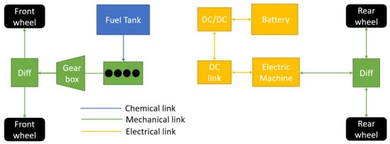
Figure 1.
Powertrain layout e-type of link between components.
The front axle was equipped with 2L diesel ICE, with a maximum power of 120 kW. The power was transferred firstly via the clutch to a six-speed automatic gearbox and secondly to the differential linked with the front wheels. The numerical modelling of the ICE follows a map-based approach. The instantaneous fuel consumption and efficiency map presented in [32], as well as the ICE’s maximum torque profile, were extracted using a web tool [33]. Figure 2 shows the instantaneous consumption and efficiency maps and the ICE maximum torque curve.
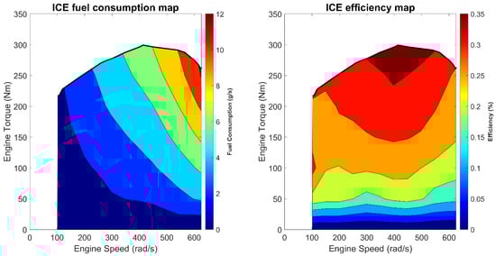
Figure 2.
ICE fuel consumption and efficiency at different operating points.
The passenger car’s gearbox was a six-speed automatic transmission, and the shift strategy refers to vehicle longitudinal speed. Table 1 shows the gearbox and differential unit transmission ratios, and the shifting speed according to vehicle velocity.

Table 1.
Transmission parameters and shifting strategy.
A permanent magnet synchronous motor (PMSM) was the EM which provides and receives power from the rear differential unit, which was modelled as a single transmission ratio. The differential unit was mechanically linked to the rear wheel, so the PMSM could provide traction force to, or recover energy from, the rear wheels. In addition, the numerical modelling of the EM followed the map-based approach, and its characteristic map, that defines the torque boundaries and operating efficiency, is shown in Figure 3.
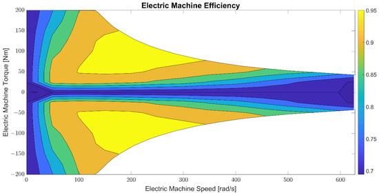
Figure 3.
Electric Machine efficiency.
The EM, whose nominal operating voltage is 700 V, was electrically connected to the Li-ion battery pack through a bi-directional power inverter. Due to the quasi-static nature of the model, the inverter was considered as a static component able to raise the DC line voltage. Therefore, the inverter’s efficiency was combined with the battery’s and shown in Figure 4. The efficiency was maximum at low power values. It decreased as the power increased, with a different rate depending on the power sign and the batteries’ state of charge.
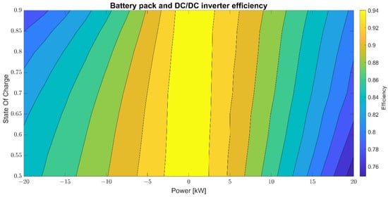
Figure 4.
Battery pack and DC/DC inverter efficiency.
2.1. Battery Mathematical Model
The modified Shepherd model (MSM) evaluates the voltage variation at the battery terminals. This MSM also presents the polarization resistance and voltage in comparison with the classical Shepherd model. These two terms allow the mathematical shaping of the dynamic phenomena involving the battery during its use. In the MSM, proposed in [34], the evolution of the battery voltage during the discharge and the charge is described through Equations (1) and (2) respectively:
In which the term is the polarization voltage, and the term the polarization resistance. The other terms are the battery current (ib), the filtered current (), the exponential zone amplitude (Ab) and the exponential zone time constant inverse (Bb).
The filtered current can be assumed to be equal to the battery current, since stationary conditions are not considered in this study. Equations (1) and (2) do not consider the aging phenomena that usually affect the battery in its life cycle. In [35], an approach based on material fatigue was carried out to determine battery degradation. The battery degradation is caused by the formation of a solid-electrolyte interphase (SEI) in the negative electrode, which competes with reversible lithium intercalation. The high rate of charging or discharging current, the high value of the depth of discharge (DOD), and the operating temperature may accelerate the degradation due to accelerated growth of the SEI. For these reasons, a stress factor was considered for each of these variables. Equation (3) evaluates the stress factor , for each cycle n that involves the depth of discharge:
where DODref is equal to a full discharge, DOD(n) is the current cycle depth of discharge, and is the stress exponent related to the depth of discharge. Similarly, the impact of the C-rate of charge and discharge current is also evaluated through Equations (4) and (5), respectively:
where IChargeref and IDischref represent the reference currents for battery stress evaluation in charge and discharge, while IChargeavg(n) and IDischargeavg(n) represent the average charge and discharge currents for the cycle n. The terms and are the stress exponents of the charge and discharge currents.
The stress factor related to operating temperature is described by Equation (6), where Ta(n) and Tref are the operating temperatures during the cycle n and the reference temperature for battery degradation assessment, and φ is the Arrhenius constant.
The product of all the stress factors is equal to the stress experienced by the battery for each cycle [36]. The maximum number of cycles (Nc) until a certain level of degradation is inversely proportional to the resulting stress factor, as reported in Equation (7) [37]:
In Equation (7), NCref represents the number of cycles to the end of the battery life when subjected to charge and discharge cycles, with a value of DOD = DODRef, ICharge = IChargeRef, IDisch = IDischRef and Ta = TRef. The term θ(n) is the product of all stress factors, and it is evaluated by Equation (8):
For realistic load profiles, it is rare that the battery starts and finishes every cycle with the same SOC value, which makes consecutive cycles not directly comparable in terms of DOD achieved. It is necessary to consider the equivalent number of cycles performed by the battery. This quantity can be evaluated by Equation (9). Equation (9) normalizes the partial discharge and charge of each cycle against a reference charge or discharge, which corresponds to a full discharge and charge of the battery.
The ratio between the number of cycles to end of life (Nc) and the number of equivalent cycles (Neq) defines the degradation index. Clearly, as the number of cycles increases, the index will also evaluate the cumulative degradation up to that point. The degradation index is given by Equation (10).
The degradation index, as it is defined, measures the relationship between the instantaneous capacity and the end-of-life capacity, as well as the instantaneous resistance and the end-of-life resistance, as expressed by Equations (11) and (12):
where QBOL and QEOL represent the capacity of the non-degraded battery and end-of-life battery, respectively. Similarly, RBOL and REOL represent the non-degraded and end-of-life battery resistance. Typically, the QEOL is equal to 0.8QBOL, but instead REOL is equal to 1.2 RBOL. The exponents α and β are the capacity and resistance degradation exponents of the cell. The values of α and β, as well as the values of ρ, γ1, γ2, and ϕ are calculated by performing specific laboratory tests in which the battery is degraded under controlled load conditions. The value of the constants for the cell, presented in Table 2, have been defined by Li et al. in [32] for MSM, and by Motapon et al. in [35] for an aging model.
Table 2.
Battery parameters.
2.2. Calculation of the Driving Forces
Figure 5 shows the scheme of the mathematical model. Starting from a driving cycle, the numerical model extracts the necessary information to evaluate the resistant forces for the longitudinal motion of the vehicle. It is possible to calculate the total power to execute the driving cycle by knowing the force and the desired speed. The control unit distributes the necessary power both to the front and the rear axles, managing the necessary torques to the electric machine and to the ICE.
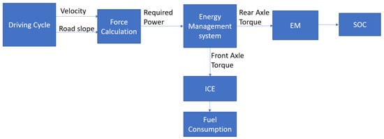
Figure 5.
Numerical model workflow.
The total amount of resistance force is equivalent to the sum of the aerodynamic resistance force, the rolling resistance, the gradient loading, and the acceleration’s inertia. To evaluate the aerodynamic resistance force, AVL CruiseTM M refers to Equation (13):
where ρa is the air density, CD is the drag coefficient, A is the vehicle’s frontal area and v is the longitudinal velocity. To evaluate the rolling resistance force, for each wheel, AVL CruiseTM M refers to Equation (14):
where Fw is the vertical load acting on the wheel and cw is the rolling resistance factor. Li et al. [32] considered the total rolling resistance force as a constant force of 70 N, named Fr*, acting on the vehicle (four wheels). To obtain the same result in CruiseM, considering that Equation (14) refers to one wheel, cw has to be calculated by Equation (15):
To evaluate the gradient loading, AVL CruiseTM M refers to Equation (16):
where is the vehicle mass, g is the gravity acceleration and αr is the road inclination angle. The inertia force is evaluated by Equation (17):
Thrust force is the sum of the resistance force (13–17). The total torque for the traction, which must be provided to the two axles, is the product of thrust force and the wheels’ rolling radius, as expressed by Equation (18):
where Ctot is the total necessary torque, considered as the sum of front axle torque (Cf) and rear axle torque (Cr), and Rw is the wheels’ rolling radius. Table 3 shows the values of the parameters for Equations (15)–(18) with reference to the considered vehicle.
Table 3.
Resistance force parameters [32].
2.3. Front and Rear Axle Torque, Speed, and Power
The EMS, depending on the vehicle’s actual state, manages the Cf and the Cr, and therefore the torque requested by the ICE and EM. Cf, which depends on CICE, can only be positive, while Cr, which depends on CEM, can be positive (motor) or negative (generator). ICE torque, angular velocity and requested power are evaluated by Equations (19)–(21):
where τFFD is the front final drive transmission ratio, τGB is the gear box transmission ratio, ηGB is the gear box efficiency and ηFFD is the front final drive efficiency. PICE is the ICE power, the product of its angular velocity (ωICE) and torque (CICE). The instantaneous torque and angular velocity, in accordance with Figure 2, define the instantaneous fuel consumption.
Equations (22)–(24) are defined to evaluate the electric machine-requested torque, speed, and power:
where is the requested torque to the electric machine from EMS, τRFD is the rear final drive transmission ratio, and ηRFD is the real axle final drive efficiency. The sign of the efficiency exponent depends on the operating conditions of the EM. When EM operates as a motor (positive power), it has to overcome energy losses in the final reducer, so the efficiency divides the torque. Otherwise, EM operating as a generator can only absorb the power not dissipated within the final reducer, so the efficiency multiplies the torque. The product between the requested torque and EM angular velocity (ωEM) returns the electric machine power (PEM).
PEM is mechanical power that is converted into electrical power from the EM to the battery pack. Equation (25) estimates the electrical power required (or supplied) to the battery:
where PB is the electrical power required (or supplied) to the battery, ηEM is the EM efficiency (Figure 3), ηEB is the battery efficiency (Figure 4) and ηPE is the AC/DC inverter and DC line efficiency. When the electric machine is running as a motor and requires PEM, the battery provides PEM with the contribution of the power dissipated in the electronic components (the efficiencies divide PEM). When the electric machine provides PEM, a part of this power is dissipated into the electronic components, so the efficiencies multiply PEM. In Equation (21), the term −1 comes from the sign convention used for batteries (negative power for discharge, positive power for recharge). Table 4 collects the powertrain efficiencies not involved in the maps already shown. The values have been presented by Li et al. in [32].
Table 4.
Powertrain efficiency.
3. Validation Procedure
Li et al. [32] presented the results obtained by their numerical model in different scenarios. A simulation with the same scenario presented in Li et al.’s study was conducted to compare the result between their model (the reference) and the AVL CruiseM model. SOC and the vehicle’s power evolution were compared after setting the same driving cycle as input, as well as the same energy management strategy. Figure 6 shows the comparison between the reference model’s power profile and the simulated model, and the vehicle speed profile compared with WLTC medium section velocity. The vehicle’s speed perfectly overlaps the driving cycle, indicating the correctness of the equations discussed. The comparison of the power time histories confirms that the developed numerical model power strictly matches the reference model, which means that the evaluation of the torques necessary to the motion of the simulated car is congruent with those used in the reference model.
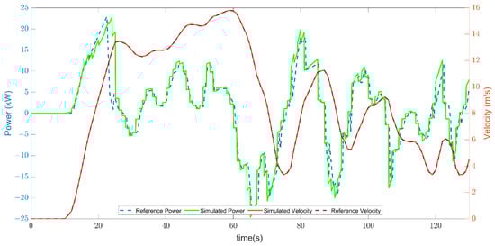
Figure 6.
Power and speed time series analyzed during the validation procedure.
Figure 7 shows the time evolution of battery SOC for the developed model and the reference model. SOC is closely related to the efficiency of the electronic components. Li et al. in [32] illustrated the evolution of the battery state of charge when the charge-sustaining operation mode is active. In this operation mode, the control system acts to maintain the battery state of charge around a predefined value (in this case SOC = 60%). The trend of the simulated SOC is comparable with the reference one, indicating the correct modelling of the control system and electrical components efficiency map. Figure 7 also shows the relative percent error between the two curves.
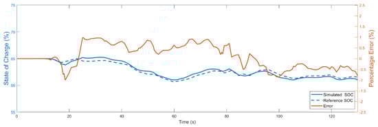
Figure 7.
Evolution of the compared SOC and relative percentage error.
The relative percentage error between the two curves confirms that the numerical model properly describes the vehicle behavior, being always less than ± 1%. Table 5 collects the data relative to the measurements of the percentage error.
Table 5.
Error between reference SOC and proposed model SOC.
4. The Energy Management System
This paper proposes the study and the evaluation of the performance of an energy management system in terms of fuel economy and battery degradation. The energy management strategy is based on a rule-based approach. This kind of approach allows a suitable implementation in a vehicle, and its efficiency, after optimization, is equivalent to EMS based on a neural network or dynamic programming [38,39]. The layout of the proposed EMS is shown in Figure 8:
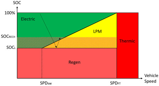
Figure 8.
Operating modes of the proposed EMS.
In which the x-axis is the vehicle velocity, and the y-axis is the state of charge of the battery. For each value of the vehicle’s longitudinal velocity and battery state of charge, it is possible to define an operational mode that determines the amount of power required by the ICE and EM. In detail:
- -
- Full Electric mode: all the traction is provided by the electric machine that drains energy from the battery.
- -
- Load Point Moving (LPM) mode: ICE delivers constant torque (Tc). If the engine power exceeds the driving cycle request, the electric machine operates as a generator and converts the excess mechanical power into electric recharging power. Otherwise, if the engine power is less than the driving cycle request, the electric machine operates as a motor and supplies the missing power.
- -
- Full Thermic: all the traction is demanded to the internal combustion engine; no electrical power is allowed to avoid overspeed of the electric machine.
- -
- Recharging mode: if the battery state of charge reaches its lower limit value, the energy management system actuates the recharging mode. The ICE torque command is the minimum among:
- Ctot plus its twenty percent value (considered at the clutch node)
- Maximum ICE available traction torque
- Maximum EM available generator torque
This operating mode is maintained until the battery reaches the SOCrecharging value, to avoid the battery operating in a critical and unsafe zone.
- -
- Braking: during the braking phases it is assumed that the total braking force is demanded by the rear axle, which is connected to the electric machine and can operate regenerative braking. The rear axle braking torque is saturated at the generator torque boundaries.
Figure 8 shows that EMS is defined by the value of the parameters SPDsw, SPDFT, SOCL, SOCRECH and TC. The parameters’ values can substantially change the operation of the vehicle and the ability to achieve the different operating modes. The study investigates the effect of torque delivered by the engine in the LPM mode in terms of fuel economy and battery degradation. The value of TC is subject to definition, while the value of the other calibration constants is defined by the authors’ experience, but subject to optimization in future work.
Table 6 collects all the EMS parameters and their meaning:
Table 6.
EMS parameters.
At the end of a simulated driving cycle, the vehicle has used a certain amount of fuel and the battery SOC has reached the SOC final value, which is usually different from the initial SOC. By determining the equivalence between the SOC variation and the fuel, it is possible to evaluate the “electrical fuel” that, added to the fuel consumed by the thermal engine, gives the real fuel value, considered as the reference for the driving cycle.
For the evaluation of electrical fuel consumption, it was assumed that all the recharge energy comes only from the ICE, not considering the regenerative braking. The final state of charge, which is used to calculate equivalent average consumption, inherently considers any energy input due to regenerative braking. Not considering regenerative braking will also place the study under more conservative conditions when calculating fuel economy.
It is assumed that the ICE power flows through the transmission components, reaching the electric machine, which transforms the mechanical energy into electrical energy for recharging the battery pack. The scheme of power flow is shown in Figure 9.
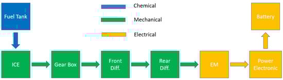
Figure 9.
Recharging power flow, from ICE to EM.
When the final SOC is less than the initial SOC, this means that a smaller amount of energy is available compared to the starting instance, so the ICE must restore the battery SOC, consuming fuel. The fuel consumed for recharging the battery (electrical fuel) will be added to the fuel consumed during the trip. Otherwise, it will be subtracted. To evaluate the electric fuel consumption, Equation (26) must be referred to:
where Vn is the nominal battery voltage, C is the battery capacity, SOCi is the battery state of charge at the beginning of the trip and SOCf is the final state of charge. EElectric represents the electrical energy consumed (when ∆SOC is positive), or absorbed (when ∆SOC is negative), by the electric machine. Assuming that the power is provided only by the ICE, Equation (27) is as follows:
where PICE is the power provided by the ICE for recharging the battery pack, ηGB is the gearbox efficiency, ηFDiff is the front differential unit efficiency, ηRDiff is the rear differential unit efficiency, ηPE is the DC line efficiency and ηBatt is the battery and inverter efficiency (Figure 4).
The instantaneous fuel consumption for an internal combustion engine is expressed by Equation (28):
in which LHV is the low heating value of diesel fuel (44.4 MJ/kg) and ηICE is the internal combustion engine efficiency. By replacing Equation (28) with Equation (27), Equation (29) can be obtained:
in which ηtot collects all the efficiencies already presented, as in Equation (30):
Integrating Equation (29) and knowing the total electrical energy from Equation (26), it is possible to evaluate the electrical fuel consumption, mELfuel, by obtaining Equation (31):
The fuel consumption used to determine the efficiency of the EMS is the sum of the ICE fuel consumption and the electrical fuel consumption (31), obtaining the real fuel consumed described in the Equation (32):
mRealfuel value is closely related to the optimization of the working points of the ICE and EM. This paper intends to identify the TC value which minimizes mRealfuel value for urban routes driven in the city of Messina and correlate it with the battery degradation. The values of the other parameters presented in Table 6 (SPDsw, SPDFT, SOCL, SOCRECH) are assumed to be optimal in terms of fuel economy in this work, but they will be subject to optimization processes in future work.
5. Experimental Driving Cycles
Two specific paths, located in Messina (Sicily, Italy), were chosen to test the numerical model. Figure 10 shows the most important roads crossing Messina’s city centre according to the classification of OpenStreetMap [40] and the proposed paths.
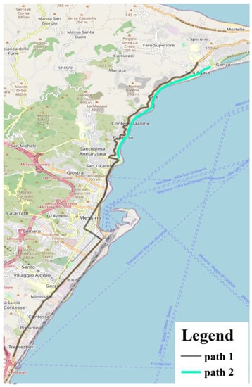
Figure 10.
The base map of the city centre of Messina with the proposed paths.
The two proposed paths presented different territorial parameters, as reported in Table 7. The roads’ parameters were extracted from the OpenStreetMap database and intersected with the specific paths in a GIS environment (Arcgis 10.x). Path 1 is the longest at 17.19 km, almost three times the length of path 2 at 5.84 km. It may be considered an extra-urban path as it is composed of 84% primary roads and only 16% other roads (secondary, tertiary, and residential roads). Path 2 is made up of residential and secondary roads (almost 98%) and may be considered an urban path. To create experimental driving cycles (DCs), a GPS unit equipped with the “TrackAddict” application was used for all paths, and data such as instantaneous speed, acceleration, latitude, longitude and altitude were collected at a frequency of 1 Hz. Kinematic parameters are shown in Table 7. The product of speed and acceleration, calculated when acceleration was positive, is proportional to vehicle power. The driving cycle of path 1, probably because of its uncongested roads, presents more stable values in terms of speeds, accelerations, and product v*a than path 2.
Table 7.
The main kinetic and territorial parameters of experimental driving cycles.
In order to obtain reliable road gradients, the altitudes collected with a GPS unit were compared with those extracted from topographic maps obtained by aerial photogrammetric measurements with an average offset of 10%. This provided realistic slope values useful for the model inputs. An overview of speed profiles and altitude profiles is reported in Figure 11.
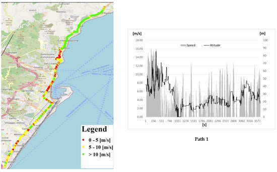
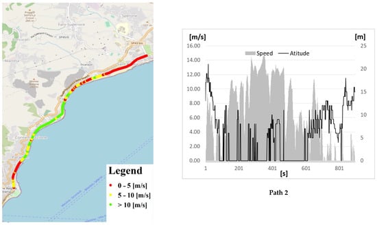
Figure 11.
Speed and altitude profiles for all proposed experimental driving cycles.
6. Results
The control system efficiency was tested by evaluating the fuel consumption at two varying parameters (TC and SOCi) for the two proposed driving cycles. For each driving cycle, different scenarios were evaluated in terms of fuel consumption, considering the following parameters:
- -
- the TC torque from 50 Nm to 120 Nm with steps of 10 Nm;
- -
- the initial state of charge assuming the values of 100%, 65%, and 30%.
The results show that the best result in terms of consumption economy was when TC was approximately equal to 90 Nm. The engine speed was, on average, 200 rad/s due to the imposed shift strategy and the urban nature of the driving cycles. The ICE efficiency map (Figure 2) shows an increase in efficiency as torque increased at 200 rad/s, while Figure 4 shows a reduction of the battery and inverter efficiency as recharging power increased. Instantaneous fuel consumption (Figure 2) always increases as engine power increases. The concatenation of these three factors results in the best fuel economy at 90 Nm; on average, all other parameters being equal as reported in Figure 12.
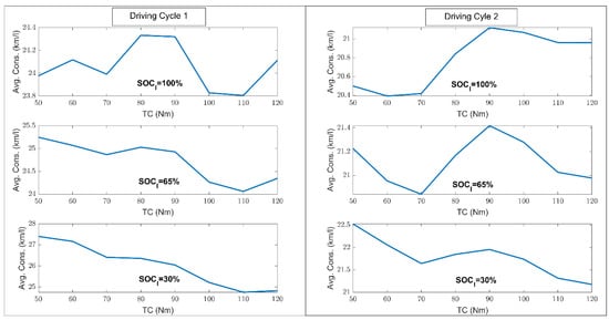
Figure 12.
Equivalent fuel consumption of each simulated scenario.
Figure 13 shows the number of cycles at the end-of-life of the battery when subjected to a load cycle typical of the execution of path 1. The x-axis shows the value of TC torque, while the y-axis shows the duration ratio. Duration ratio means the ratio of the distance traveled until the end-of-life capacity of the batteries is reached in different cases to the maximum distance traveled in the best case, i.e., XXX km.
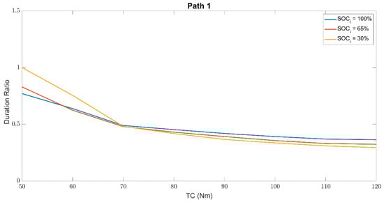
Figure 13.
Battery equivalent number of cycles to end of life during the execution of path 1.
Figure 13 demonstrates a progressive deterioration of the battery as the constant torque TC increases. When the charging torques and current are low, the battery is less subject to deterioration; as the charging torques increase, the battery presents a greater deterioration as the charging factor grows.
The figure also shows that SOCi affects the end-of-life battery cycles; for low TC values, when SOCi is 30%, the battery aging is less onerous than when the SOCi is 65% and even less for SOCi 100%. This phenomenon suggests that the full-electric mode is more stressful for the battery than the hybrid one, especially for low-charging torques. A fully charged battery covers a longer distance in full-electric mode (or charge-depleting mode) than a lower battery SOC. Given the average cycle speeds (about 17 km/h), the v*a value (1.63 m2/s3) and considering that the cycle took place mainly on primary roads, it can be concluded that the exclusive use of the battery (full electric mode) affects its end of life more than hybrid mode. Low SOCi and low TC values mean that, in hybrid mode, the torque delivered by the ICE is used almost entirely for traction, which means that the electric motor demands or delivers small amounts of current to the battery. As TC charging torque increases, the battery is more stressed, and this thesis is supported by the fact that at TC = 70 Nm the trend between the hybrid and the electric mode is reversed. Before 70 Nm, the SOCi is the parameter with more influence on the battery aging (and so the distance travelled in full electric mode), but from a TC equal to 70 Nm torque itself becomes the most damaging parameter for the battery.
Figure 14 shows the results of path 2, and the trends confirm the previous assumptions. For path 2, the maximum distance traveled in the best case is XXX km.
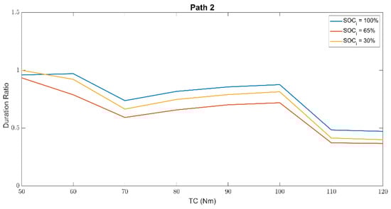
Figure 14.
Battery equivalent number of cycles to end of life during the execution of path 2.
The average cycle speeds are higher (23 km/h), as is the value of v*a (2.42 m2/s2). This results in two conclusions:
- (1)
- The average speed of cycle 2 causes the control system to command the hybrid mode more often than in driving cycle 1.
- (2)
- The value of v*a suggests that, on average, more traction power is required from the car in cycle 2 than in cycle 1.
Again, two critical aspects concur in battery aging, such as the traveled distance in full electric mode and the TC value. For low TC values, lower SOCi values are less stressful for the battery than higher ones. As torque increases, the trend changes. Given the higher average torque demands than before, the trend is also more constant. The balance between the stress caused by full-electric mode and the stress due to TC torque is reached between 90 and 100 Nm.
7. Conclusions
The proposed paper aimed at investigating and implementing a rule-based energy management system for hybrid vehicles by considering instantaneous fuel consumption and battery aging. The proposed methodology was implemented in AVL CRUISETM M and simulations were implemented on real driving cycles based on two different paths located in Messina (Italy). The control system efficiency was tested by varying two main parameters, such as TC and SOCi. The main results are as follows:
- The ICE efficiency is generally proportional to the TC, but the degradation of the battery is affected mostly by the recharging power;
- If analyzing the trend of the instantaneous fuel consumption, the variation of TC provides the main contribution and its trend does not considerably change from one cycle to the other;
- If analyzing the trend of battery degradation, the variation of TC gives different results and the specific paths with its typical kinematic parameters affect the battery aging itself much more.
For future works, the proposed methodology can be better developed by considering different paths, chosen with rigorous methods that could highlight the contributions of territorial and kinematic constraints to battery aging. Future studies could also involve the influence of other calibration parameters, as well as any variations in behavior on suburban roads and highways.
Author Contributions
Conceptualization, A.G., S.B. and F.F.; methodology, A.G., S.B., F.F. and U.P.; software, U.P.; writing—original draft preparation, A.G., S.B., F.F. and U.P.; writing—review and editing, A.G., S.B., F.F. and U.P.; supervision, A.G. and S.B. All authors have read and agreed to the published version of the manuscript.
Funding
This research received no external funding.
Institutional Review Board Statement
Not applicable.
Informed Consent Statement
Not applicable.
Data Availability Statement
Data sharing is not applicable.
Acknowledgments
The authors are grateful to AVL Italia for providing the simulation suites, including AVL Cruise-M. They are pleased to collaborate with the company and to be able to exchange information and expertise.
Conflicts of Interest
The authors declare no conflict of interest.
References
- Minh, V.T.; Moezzi, R.; Cyrus, J.; Hlava, J. Optimal Fuel Consumption Modelling, Simulation, and Analysis for Hybrid Electric Vehicles. Appl. Syst. Innov. 2022, 5, 36. [Google Scholar] [CrossRef]
- Dingel, O.; Ross, J.; Trivic, I.; Cavina, N.; Rioli, M. Model-Based Assessment of Hybrid Powertrain Solutions. In Proceedings of the SAE Technical Papers; SAE International: Warrendale, PA, USA, 2011. [Google Scholar]
- Previti, U.; Brusca, S.; Galvagno, A. Passenger Car Energy Demand Assessment: A New Approach Based on Road Traffic Data. In E3S Web of Conferences; EDP Sciences: Les Ulis, France, 2020; Volume 197. [Google Scholar]
- Cucinotta, F.; Raffaele, M.; Salmeri, F. A Well-to-Wheel Comparative Life Cycle Assessment between Full Electric and Traditional Petrol Engines in the European Context; Springer: Berlin/Heidelberg, Germany, 2021; ISBN 9783030705657. [Google Scholar]
- Chan, C.C. The State of the Art of Electric, Hybrid, and Fuel Cell Vehicles. Proc. IEEE 2007, 95, 704–718. [Google Scholar] [CrossRef]
- Un-Noor, F.; Padmanaban, S.; Mihet-Popa, L.; Mollah, M.N.; Hossain, E. A Comprehensive Study of Key Electric Vehicle (EV) Components, Technologies, Challenges, Impacts, and Future Direction of Development. Energies 2017, 10, 1217. [Google Scholar] [CrossRef]
- Lee, Y.; Kim, C.; Shin, J. A Hybrid Electric Vehicle Market Penetration Model to Identify the Best Policy Mix: A Consumer Ownership Cycle Approach. Appl. Energy 2016, 184, 438–449. [Google Scholar] [CrossRef]
- Ehsani, M.; Singh, K.V.; Bansal, H.O.; Mehrjardi, R.T. State of the Art and Trends in Electric and Hybrid Elec-tric Vehicles. Proc. IEEE 2021, 109, 967–984. [Google Scholar] [CrossRef]
- Zhang, P.; Yan, F.; Du, C. A Comprehensive Analysis of Energy Management Strategies for Hybrid Electric Vehicles Based on Bibliometrics. Renew. Sustain. Energy Rev. 2015, 48, 88–104. [Google Scholar] [CrossRef]
- Kim, M.; Jung, D.; Min, K. Hybrid Thermostat Strategy for Enhancing Fuel Economy of Series Hybrid Intrac-ity Bus. IEEE Trans. Veh. Technol. 2014, 63, 3569–3579. [Google Scholar] [CrossRef]
- Wang, E.; Ouyang, M.; Zhang, F.; Zhao, C. Performance Evaluation and Control Strategy Comparison of Su-percapacitors for a Hybrid Electric Vehicle. In Science, Technology and Advanced Application of Supercapacitors; IntechOpen: London, UK, 2019. [Google Scholar]
- Zhao, Z.; Yu, Z.; Yin, M.; Zhu, Y. Torque Distribution Strategy for Single Driveshaft Parallel Hybrid Electric Vehicle. In Proceedings of the 2009 IEEE Intelligent Vehicles Symposium, Xi’an, China, 3–5 June 2009; pp. 1350–1353. [Google Scholar]
- Yang, C.; Zha, M.; Wang, W.; Liu, K.; Xiang, C. Efficient Energy Management Strategy for Hybrid Electric Vehicles/Plug-in Hybrid Electric Vehicles: Review and Recent Advances under Intelligent Transportation System. IET Intell. Transp. Syst. 2020, 14, 702–711. [Google Scholar] [CrossRef]
- Song, K.; Li, F.; Hu, X.; He, L.; Niu, W.; Lu, S.; Zhang, T. Multi-Mode Energy Management Strategy for Fuel Cell Electric Vehicles Based on Driving Pattern Identification Using Learning Vector Quantization Neural Network Algorithm. J. Power Sources 2018, 389, 230–239. [Google Scholar] [CrossRef]
- Rajput, D.; Herreros, J.M.; Innocente, M.S.; Schaub, J.; Dizqah, A.M. Electrified Powertrain with Multiple Planetary Gears and Corresponding Energy Management Strategy. Vehicles 2021, 3, 341–356. [Google Scholar] [CrossRef]
- Liu, H.; Wang, C.; Zhao, X.; Guo, C. An Adaptive-Equivalent Consumption Minimum Strategy for an Extended-Range Electric Bus Based on Target Driving Cycle Generation. Energies 2018, 11, 1805. [Google Scholar] [CrossRef]
- Galvagno, A.; Previti, U.; Famoso, F.; Brusca, S. An Innovative Methodology to Take into Account Traffic Information on WLTP Cycle for Hybrid Vehicles. Energies 2021, 14, 1548. [Google Scholar] [CrossRef]
- Vu, T.M.; Moezzi, R.; Cyrus, J.; Hlava, J.; Petru, M. Parallel Hybrid Electric Vehicle Modelling and Model Pre-dictive Control. Appl. Sci. 2021, 11, 10668. [Google Scholar] [CrossRef]
- Qiang, P.; Wu, P.; Pan, T.; Zang, H. Real-Time Approximate Equivalent Consumption Minimization Strategy Based on the Single-Shaft Parallel Hybrid Powertrain. Energies 2021, 14, 7919. [Google Scholar] [CrossRef]
- Pérez, W.; Tulpule, P.; Midlam-Mohler, S.; Rizzoni, G. Data-Driven Adaptive Equivalent Consumption Minimization Strategy for Hybrid Electric and Connected Vehicles. Appl. Sci. 2022, 12, 2705. [Google Scholar] [CrossRef]
- Pei, D.; Leamy, M.J. Dynamic Programming-Informed Equivalent Cost Minimization Control Strategies for Hybrid-Electric Vehicles. J. Dyn. Syst. Meas. Control. Trans. ASME 2013, 135, 051013. [Google Scholar] [CrossRef]
- Vidal-Naquet, F.; Zito, G. Adapted Optimal Energy Management Strategy for Drivability. In Proceedings of the 2012 IEEE Vehicle Power and Propulsion Conference, VPPC 2012, Seoul, Korea, 9–12 October 2012; pp. 358–363. [Google Scholar]
- Inuzuka, S.; Zhang, B.; Shen, T. Real-Time Hev Energy Management Strategy Considering Road Congestion Based on Deep Reinforcement Learning. Energies 2021, 14, 5270. [Google Scholar] [CrossRef]
- Meng, J.; Luo, G.; Ricco, M.; Swierczynski, M.; Stroe, D.I.; Teodorescu, R. Overview of Lithium-Ion Battery Modeling Methods for State-of-Charge Estimation in Electrical Vehicles. Appl. Sci. 2018, 8, 659. [Google Scholar] [CrossRef]
- Campagna, N.; Castiglia, V.; Miceli, R.; Mastromauro, R.A.; Spataro, C.; Trapanese, M.; Viola, F. Battery Models for Battery Powered Applications: A Comparative Study. Energies 2020, 13, 4085. [Google Scholar] [CrossRef]
- Cignini, F.; Genovese, A.; Ortenzi, F.; Alessandrini, A.; Berzi, L.; Pugi, L.; Barbieri, R. Experimental Data Comparison of an Electric Minibus Equipped with Different Energy Storage Systems. Batteries 2020, 6, 26. [Google Scholar] [CrossRef]
- Padovani, T.M.; Debert, M.; Colin, G.; Chamaillard, Y. Optimal Energy Management Strategy Including Battery Health through Thermal Management for Hybrid Vehicles. In IFAC Proceedings Volumes (IFAC-PapersOnline); IFAC Secretariat: Laxenburg, Austria, 2013; Volume 7, pp. 384–389. [Google Scholar]
- Tang, L.; Rizzoni, G. Energy Management Strategy Including Battery Life Optimization for a HEV with a CVT. In Proceedings of the 2016 IEEE Transportation Electrification Conference and Expo, Asia-Pacific, ITEC Asia-Pacific 2016, Busan, Korea, 1–4 June 2016; Institute of Electrical and Electronics Engineers Inc.: Piscataway, NJ, USA, 2016; pp. 549–554. [Google Scholar]
- Atalay, S.; Sheikh, M.; Mariani, A.; Merla, Y.; Bower, E.; Widanage, W.D. Theory of Battery Ageing in a Lith-ium-Ion Battery: Capacity Fade, Nonlinear Ageing and Lifetime Prediction. J. Power Sources 2020, 478, 229026. [Google Scholar] [CrossRef]
- Dos Reis, G.; Strange, C.; Yadav, M.; Li, S. Lithium-Ion Battery Data and Where to Find It. Energy AI 2021, 5, 100081. [Google Scholar] [CrossRef]
- Tang, X.; Liu, K.; Li, K.; Widanage, W.D.; Kendrick, E.; Gao, F. Recovering Large-Scale Battery Aging Dataset with Machine Learning. Patterns 2021, 2, 100302. [Google Scholar] [CrossRef]
- Li, X.; Evangelou, S.A. Torque-Leveling Threshold-Changing Rule-Based Control for Parallel Hybrid Electric Vehicles. IEEE Trans. Veh. Technol. 2019, 68, 6509–6523. [Google Scholar] [CrossRef]
- WebPlotDigitizer. Available online: https://automeris.io/WebPlotDigitizer/ (accessed on 10 January 2022).
- Motapon, S.N.; Lupien-Bedard, A.; Dessaint, L.A.; Fortin-Blanchette, H.; Al-Haddad, K. A Generic Electro-thermal Li-Ion Battery Model for Rapid Evaluation of Cell Temperature Temporal Evolution. IEEE Trans. Ind. Electron. 2017, 64, 998–1008. [Google Scholar] [CrossRef]
- Motapon, S.N.; Lachance, E.; Dessaint, L.A.; Al-Haddad, K. A Generic Cycle Life Model for Lithium-Ion Bat-teries Based on Fatigue Theory and Equivalent Cycle Counting. IEEE Open J. Ind. Electron. Soc. 2020, 1, 207–217. [Google Scholar] [CrossRef]
- Smith, K.; Earleywine, M.; Wood, E.; Neubauer, J.; Pesaran, A. Comparison of Plug-in Hybrid Electric Vehicle Battery Life across Geographies and Drive Cycles. In Proceedings of the SAE Technical Papers; SAE International: Warrendale, PA, USA, 2012. [Google Scholar]
- Laresgoiti, I.; Käbitz, S.; Ecker, M.; Sauer, D.U. Modeling Mechanical Degradation in Lithium Ion Batteries during Cycling: Solid Electrolyte Interphase Fracture. J. Power Sources 2015, 300, 112–122. [Google Scholar] [CrossRef]
- Jeoung, H.; Lee, K.; Kim, N. Methodology for Finding Maximum Performance and Improvement Possibility of Rule-Based Control for Parallel Type-2 Hybrid Electric Vehicles. Energies 2019, 12, 1924. [Google Scholar] [CrossRef]
- Zhou, H.; Xu, Z.; Liu, L.; Liu, D.; Zhang, L. A Rule-Based Energy Management Strategy Based on Dynamic Programming for Hydraulic Hybrid Vehicles. Math. Probl. Eng. 2018, 2018, 9492026. [Google Scholar] [CrossRef]
- Openstreetmap. Available online: https://www.openstreetmap.org/ (accessed on 10 March 2022).
Publisher’s Note: MDPI stays neutral with regard to jurisdictional claims in published maps and institutional affiliations. |
© 2022 by the authors. Licensee MDPI, Basel, Switzerland. This article is an open access article distributed under the terms and conditions of the Creative Commons Attribution (CC BY) license (https://creativecommons.org/licenses/by/4.0/).