
Quantifying the Relation between Activity Pattern Complexity and Car Use Using a Partial Least Square Structural Equation Model


Abstract
:1. Introduction
- It quantifies the relation between variables representing the complexity of activity chains with car use characteristics. Despite the chosen methodology working well with small sample sizes, socio-demographic variables need to be controlled for. Therefore, the study provides insights into the importance of socio-demographic characteristics (gender, age, family composition, etc.) on the said relationship.
- It demonstrates the robustness of PLS-SEM towards important variations in the dataset. More precisely, the quantified relations are shown to not change significantly even if all individuals have relocated their work address. Moreover, the model was calibrated on the two waves, considering all days of the individuals as uncorrelated, an acceptable assumption given the low multi-collinearity quantified in the datasets, as well as using a single day of the week. Results of the model are found to be consistent.
2. Literature Review
3. Methodology
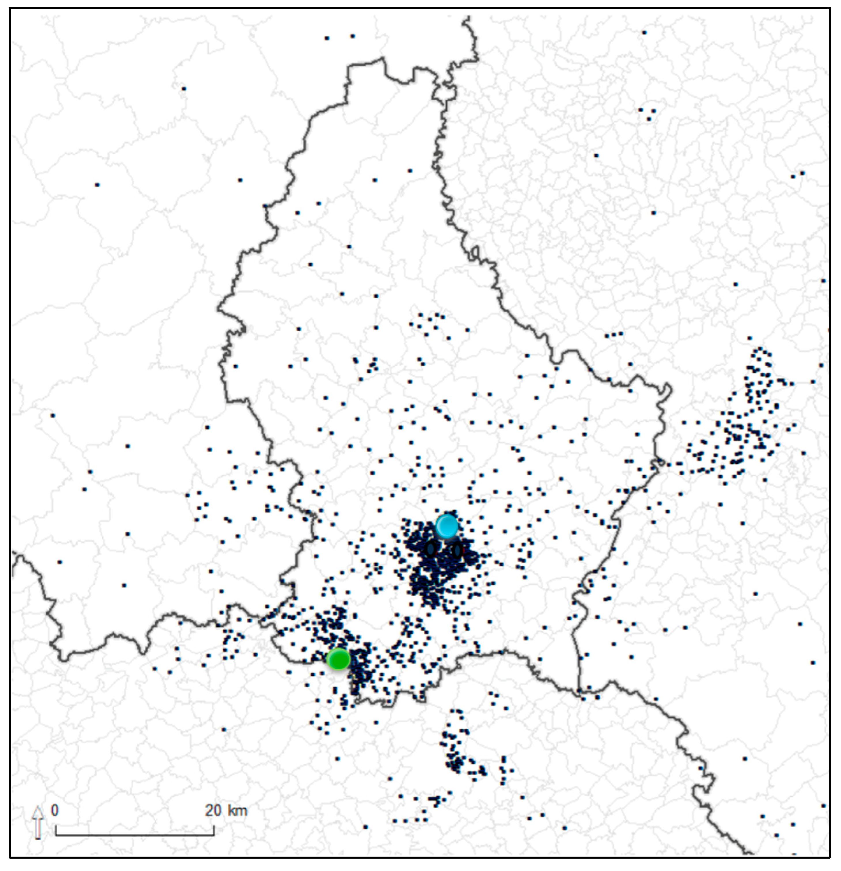
3.1. Case Study
3.2. Descriptive Analysis
3.3. PLS SEM
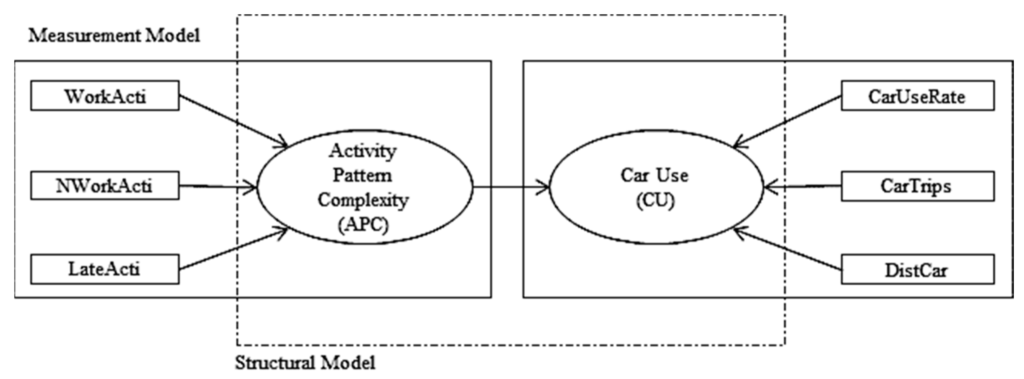
3.3.1. Model Specification
3.3.2. Model Validation
4. Results and Discussion
5. Conclusions
Author Contributions
Funding
Institutional Review Board Statement
Informed Consent Statement
Data Availability Statement
Acknowledgments
Conflicts of Interest
Appendix A. Sample Description
| Socio-Demographic Information | |||||
| Surveyed population | 51 | Administrative or technical staff | 25.5% | ||
| Male | 25.5% | Average age | 35 | ||
| PhD students | 29.4% | Presence of kids younger than 12 | 33.3% | ||
| Professors or researchers | 45.1% | Cross-borders workers | 31.3% | ||
| General statistics on the multi-day dataset | |||||
| Total days | 705 | Weekday with working activity (study day) | 444 | ||
| Average day per individual | 13.8 | Average “study day” per individual | 8.7 | ||
| Total activities | 2793 | Considered activities | 1850 | ||
| Home | 1046 | Home | 605 | ||
| Work | 565 | Work | 556 | ||
| Mobility behaviour (for study days) | |||||
| Minimum | Maximum | Average | Standard Deviation | ||
| Travel distance by car (km) | 0.0 | 779.5 | 49.7 | 79.7 | |
| Travel distance by public transport (km) | 0.0 | 724.4 | 22.3 | 68.0 | |
| Travelled distance by soft modes (km) | 0.0 | 64.9 | 1.6 | 4.5 | |
| Activity information (for study days) | |||||
| Minimum | Maximum | Average | Standard Deviation | ||
| Activities during a work day | 2 | 11 | 4.2 | 1.7 | |
| Activity time during a work day (min) | 65 | 1537 | 601 | 154 | |
| Work activity time during a work day (min) | 30 | 810 | 469 | 118 | |
| Non-work activity time during a work day (min) | 0 | 1207 | 131 | 144 | |
Appendix B. PLS-SEM Analysis with One (Average) Day / Participant (2015 Dataset)
| Path Coefficients | WorkTour | All | ||||
| Original Sample | T Stat. | p-Values | Original Sample | T Stat. | p-Values | |
| Activity Pattern Complexity -> Car Use | 0.556 | 2.3205 | * | 0.500 | 1.873 | . |
| Outer Loadings | ||||||
| Original Sample | T Stat. | p-Values | Original Sample | T Stat. | p-Values | |
| CarUsage -> CU | 0.994 | 1.629 | 0.992 | 1.571 | ||
| CarUseRate -> CU | 0.904 | 1.673 | . | 0.927 | 1.635 | |
| DistCar -> CU | 0.429 | 1.246 | 0.505 | 1.453 | ||
| LateActi -> ACP | 0.227 | 0.667 | 0.189 | 0.497 | ||
| NWorkActi -> ACP | 0.973 | 1.647 | . | 0.939 | 1.603 | |
| WorkActi -> ACP | 0.577 | 1.523 | 0.530 | 1.408 | ||
| Outer Weights | ||||||
| Original Sample | T Stat. | p-Values | Original Sample | T Stat. | p-Values | |
| CarUsage -> CU | 0.818 | 1.458 | 0.779 | 1.358 | ||
| CarUseRate -> CU | 0.236 | 1.366 | 0.229 | 1.084 | ||
| DistCar -> CU | −0.063 | 0.221 | 0.029 | 0.134 | ||
| LateActi -> APC | −0.033 | 0.135 | −0.232 | 0.602 | ||
| NWorkActi -> APC | 0.886 | 1.625 | 0.948 | 1.571 | ||
| WorkActi -> APC | 0.253 | 1.284 | 0.290 | 1.19 | ||
| Validity Criteria | ||||||
| R2 Car Use Behavior | 0.309 | 0.25 | ||||
| SRMR | 0.137 | 0.131 | ||||
| Discriminant Validity | 0.556 | 0.5 | ||||
| Significance codes: 0.01 “*”, 0.1 “.”, 1 “ ”. | ||||||
References
- Sprumont, F.; Astegiano, P.; Viti, F. On the consistency between commuting satisfaction and traveling utility: The case of the University of Luxembourg. Eur. J. Transp. Infrastruct. Res. 2017, 17, 248–262. [Google Scholar]
- Sprumont, F.; Astegiano, P.; Viti, F. Analyzing the relation between commuting satisfaction and residential choice using discrete choice theory and Structural Equation Modeling. In Proceedings of the TRB Annual Meeting, Washington, DC, USA; 2017. [Google Scholar]
- Adler, T.; Ben-Akiva, M. A theoretical and empirical model of trip chaining behavior. Transp. Res. Part B 1979, 13, 243–257. [Google Scholar] [CrossRef]
- Bhat, C. An analysis of evening commute stop-making behavior using repeated choice observations from a multi-day survey. Transp. Res. Part B 1999, 33, 495–510. [Google Scholar] [CrossRef]
- Timmermans, H.; van der Waerden, P.; Alves, M.; Polak, J.; Ellis, S.; Harvey, A.S.; Zandee, R. Spatial context and the complexity of daily travel patterns: An international comparison. J. Transp. Geogr. 2003, 11, 37–46. [Google Scholar] [CrossRef]
- Krygsman, S.; Arentze, T.; Timmermans, H. Capturing tour mode and activity choice interdependencies: A co-evolutionary logit modelling approach. Transp. Res. Part A 2007, 41, 913–933. [Google Scholar] [CrossRef]
- Golob, T.F. Structural equation modeling for travel behavior research. Transp. Res. Part B 2003, 37, 1–25. [Google Scholar] [CrossRef]
- Nicholson, A.; Kingham, S. The university of Canterbury transport strategy. In Proceedings of the 26th Australasian Transport Research Forum, Wellington, New Zealand, 1–3 October 2003. [Google Scholar]
- Andrade, K.; Kagaya, S.; Uchida, K.; Dantas, A.; Nicholson, A. A Study on the Temporal Transferability of Transport Modal Choice Models. Stud. Reg. Sci. 2007, 37, 887–899. [Google Scholar] [CrossRef]
- De Witte, A.; Hollevoet, J.; Dobruszkes, F.; Hubert, M.; Macharis, C. Linking modal choice to motility: A comprehensive review. Transp. Res. Part A 2013, 49, 329–341. [Google Scholar] [CrossRef]
- Zhou, J. Sustainable commute in a car-dominant city: Factors affecting alternative mode choices among university students. Transp. Res. Part A 2012, 46, 1013–1029. [Google Scholar] [CrossRef]
- Van Acker, V.; Witlox, F.; Van Wee, B. The effects of the land use system on travel behavior: A Structural Equation Modeling approach. Transp. Plan. Technol. 2007, 30, 331–353. [Google Scholar] [CrossRef]
- Ewing, R.; Cervero, R. Travel and the built environment. J. Am. Plan. Assoc. 2010, 76, 265–294. [Google Scholar] [CrossRef]
- Viti, F.; Tampère, C.; Frederix, R.; Castaigne, M.; Walle, F.; Cornelis, E. Analyzing Weekly Activity-Travel Behaviour from Behavioural Survey and Traffic Data. 2010. Available online: https://lirias.kuleuven.be/handle/123456789/294554 (accessed on 1 August 2022).
- Vande Walle, S.; Steenberghen, T. Space and time related determinants of public transport use in trip chains. Transp. Res. Part A 2006, 40, 151–162. [Google Scholar] [CrossRef]
- Ye, X.; Pendyala, R.M.; Gottardi, G. An exploration of the relationship between mode choice and complexity of trip chaining patterns. Transp. Res. Part B 2007, 41, 96–113. [Google Scholar] [CrossRef]
- McGuckin, N.; Zmud, J.; Nakamoto, Y. Trip-chaining trends in the US: Understanding travel behavior for policy making. Transp. Res. Rec. 2005, 1917, 199–204. [Google Scholar] [CrossRef]
- Lee, M.S.; McNally, M.G. On the structure of weekly activity/travel patterns. Transp. Res. Part A 2003, 37, 823–839. [Google Scholar] [CrossRef]
- Hensher, D.A.; Reyes, A.J. Trip chaining as a barrier to the propensity to use public transport. Transportation 2000, 27, 341–361. [Google Scholar] [CrossRef]
- Kuppam, A.R.; Pendyala, R.M. A structural equations analysis of commuters’ activity and travel patterns. Transportation 2001, 28, 33–54. [Google Scholar] [CrossRef]
- Daisy, N.S.; Millward, H.; Liu, L. Trip chaining and tour mode choice of non-workers grouped by daily activity patterns. J. Transp. Geogr. 2014, 69, 150–162. [Google Scholar] [CrossRef]
- Bautista-Hernandez, D. Urban structure and its influence on trip chaining complexity in the Mexico City Metropolitan Area. Urban Plan. Transp. Res. 2020, 8, 71–97. [Google Scholar] [CrossRef]
- Thorhauge, M.; Kassahun, H.T.; Cherchi, E.; Haustein, S. Mobility needs, activity patterns and activity flexibility: How subjective and objective constraints influence mode choice. Transp. Res. Part A 2020, 139, 255–272. [Google Scholar] [CrossRef]
- Scheffer, A.; Connors, R.; Viti, F. Trip chaining impact on within-day mode choice dynamics: Evidences from a multi-day travel survey. Transp. Res. Procedia 2021, 52, 684–691. [Google Scholar] [CrossRef]
- Md Tazul, I.; Khandker, M.N.H. Unraveling the relationship between trip chaining and mode choice: Evidence from a multi-week travel diary. Transp. Plan. Technol. 2012, 35, 409–426. [Google Scholar]
- Md Hadiuzzaman, N.P.F.; Sanjana, H.; Saurav, B.; Farzana, R. Structural equation approach to investigate trip-chaining and mode choice relationships in the context of developing countries. Transp. Plan. Technol. 2019, 42, 391–415. [Google Scholar] [CrossRef]
- Jöreskog, K.G. A general method for estimating a Linear Structural Equation System. ETS Res. Bull. Ser. 1970, 2, 1–41. [Google Scholar] [CrossRef]
- Hair, J.F.; Ringle, C.M.; Gudergard, S.P.; Fischer, A.; Nitzi, C.; Menictas, C. Partial least squares structural equation modeling-based discrete choice modeling: An illustration in modeling retailer choice. Bus. Res. 2018, 12, 115–142. [Google Scholar] [CrossRef]
- Banerjee, U.; Hine, J. Interpreting the influence of urban form on household car travel using partial least squares structural equation modelling: Some evidence from Northern Ireland. Transp. Plan. Technol. 2016, 39, 24–44. [Google Scholar] [CrossRef]
- Coltman, T.; Devinney, T.M.; Midgley, D.F.; Venaik, S. Formative versus reflective measurement models: Two applications of formative measurement. J. Bus. Res. 2008, 61, 1250–1262. [Google Scholar] [CrossRef]
- Lowry, P.B.; Gaskin, J. Partial Least Squares (PLS) Structural Equation Modeling (SEM) for building and testing behavioral causal theory: When to choose it and how to use it. IEEE Trans. Prof. Commun. 2014, 57, 123–146. [Google Scholar] [CrossRef]
- Hair, J.F.; Ringle, C.M.; Sarstedt, M. PLS-SEM: Indeed a silver bullet. J. Mark. Theory Pract. 2011, 19, 139–152. [Google Scholar] [CrossRef]
- Nguyen-Phouc, D.Q.; Oviedo-Trespalacios, O.; Nguyen, M.H.; Dinh, M.T.T.; Su, D.N. Intentions to use ride-sourcing services in Vietnam: What happens after three months without COVID-19 infections? Cities 2022, 126, 103691. [Google Scholar] [CrossRef] [PubMed]
- Nguyen-Phouc, D.Q.; Su, D.N.; Nguyen, M.H.; Vo, N.S.; Oviedo-Trespalacios, O. Factors influencing intention to use on-demand shared ride-hailing services in Vietnam: Risk, cost or sustainability? J. Transp. Geogr. 2022, 99, 103302. [Google Scholar] [CrossRef]
- Satorra, A. Robustness issues in structural equation modeling: A review of recent developments. Qual. Quant. 1990, 24, 367–386. [Google Scholar] [CrossRef]
- Yuan, K.-H.; Bentler, P.M. Robust procedures in Structural Equation Modeling. Handb. Latent Var. Relat. Models 2007, 367–397. [Google Scholar]
- Carpentier, S.; Gerber, P. Les Déplacements Domicile-travail: En Voiture, en Train ou à pied ? 2009. Available online: https://halshs.archives-ouvertes.fr/halshs-01132986/document (accessed on 1 August 2022).
- Sprumont, F.; Viti, F.; Caruso, G.; König, A. Workplace relocation and mobility changes in a transnational metropolitan area: The case of the University of Luxembourg. Transp. Res. Procedia 2014, 4, 286–299. [Google Scholar] [CrossRef]
- Sprumont, F.; Viti, F. The effect of workplace relocation on individuals’ activity travel behavior. J. Transp. Land Use 2018, 11, 985–1001. [Google Scholar] [CrossRef]
- Sprumont, F.; Benam, A.; Viti, F. Short- and long-term impacts of workplace relocation: A survey and experience from the University of Luxembourg relocation. Sustainability 2020, 12, 7506. [Google Scholar] [CrossRef]
- Vale, D.S. Does commuting time tolerance impede sustainable urban mobility? Analysing the impacts on commuting behaviour as a result of workplace relocation to a mixed-use centre in Lisbon. J. Transp. Geogr. 2013, 32, 38–48. [Google Scholar] [CrossRef]
- Ringle, C.M.; Wende, S.; Becker, J.-M. SmartPLS 3; SmartPLS GmbH: Boenningstedt, Germany, 2015; Available online: http://www.smartpls.com (accessed on 1 August 2022).
- Wong, K.K.-K. Partial Least Squares Structural Equation Modeling (PLS-SEM) Techniques Using SmartPLS. Mark. Bull. 2013, 24, 1–32. [Google Scholar]
- Marcoulides, G.A.; Saunders, C. Editor’s Comments–PLS: A silver bullet? MIS Q. 2006, 30, iii–ix. [Google Scholar] [CrossRef]
- Hair, J.F.; Hult GT, M.; Ringle, C.M.; Sarstedt, M. A Primer on Partial Least Squares Structural Equation Modeling (PLS-SEM); SAGE Publications, Inc.: Thousand Oaks, CA, USA, 2013. [Google Scholar]
- Hoyle, R.H. Structural Equation Modeling; SAGE Publications, Inc.: Thousand Oaks, CA, USA, 1995. [Google Scholar]
- Moiseeva, A.; Timmermans, H.; Choi, J.; Joh, C.-H. Sequence alignment analysis of variability in activity travel patterns through 8 weeks of diary data. Transp. Res. Rec. 2014, 2412, 49–56. [Google Scholar] [CrossRef]
- Garson, G.D. Partial Least Squares: Regression & Structural Equation Models; School of Public & International Affairs North Carolina State University: Raleigh, NC, USA, 2016. [Google Scholar]
- Cenfetelli, R.T.; Basillier, G. Interpretations of formative measurement in information systems research. MIS Q. 2009, 33, 689–708. [Google Scholar] [CrossRef]
- Hertzog, L.R. How Robust Are Structural Equation Models to Model Miss-Specification? A Simulation Study; Working Paper; University of Ghent: Ghent, Belgium, 2018; Available online: https://arxiv.org/pdf/1803.06186.pdf (accessed on 26 July 2019).
- Henseler, J.; Dijkstra, T.K.; Sarstedt, M.; Ringle, C.M.; Diamantopoulos, A.; Straub, D.W.; Ketchen, D.J.; Hair, J.F.; Hult, G.T.M.; Calantone, R.J. Common Beliefs and Reality about Partial Least Squares: Comments on Rönkkö & Evermann. Organ. Res. Methods 2014, 17, 182–209. [Google Scholar]
- Hu, L.; Bentler, P.M. Fit indices in covariance structure modeling: Sensitivity to underparameterized model misspecification. Psychol. Methods 1998, 3, 424–453. [Google Scholar] [CrossRef]
- Lu, X.; Pas, E.I. Socio-demographics, activity participation and travel behavior. Transp. Res. Part A Policy Pract. 1999, 33, 1–18. [Google Scholar] [CrossRef]
- Vanoutrive, T. Workplace travel plans: Can they be evaluated effectively by experts? Transp. Plan. Technol. 2014, 37, 757–774. [Google Scholar] [CrossRef]
- Sprumont, F. Activity-travel behaviour in the context of workplace relocation. Ph.D. Thesis, University of Luxembourg, Luxembourg, 2017. Available online: https://orbilu.uni.lu/bitstream/10993/33729/1/Sprumont%20F.%20Thesis.pdf (accessed on 1 August 2022).


| Indicators used for the car use latent variable (CU) |
|---|
| Distcar: total distance travelled by car over the whole day (All), or within work tour (Work) |
| CarTrips: number of trips done by car over the whole day (All), or within work tour (Work) |
| CarUseRate: Share of the total trip done by car over the whole day (All), or within work tour (Work) |
| Indicators used for the activity pattern complexity latent variable (APC) |
| NWorkActi: number of non-work activities performed over the whole day (All), or within work tour (Work) |
| WorkActi: number of work activities performed over the whole day (All), or within work tour (Work) |
| LateActi: number of activities started after 7 p.m. over the whole day (All), or within work tour (Work) |
| SmartPLS Results | 2016 | 2015 | ||||||||||
|---|---|---|---|---|---|---|---|---|---|---|---|---|
| ALL | Work | ALL | Work | |||||||||
| Origin. Sampl. | T Statistic | p-Values | Origin. Sampl. | T Statistic | p-Values | Origin. Sampl. | T Statistic | p-Values | Origin. Sampl. | T Statistic | p-Values | |
| Path Coefficients | ||||||||||||
| APC -> CU | 0.512 | 15.274 | *** | 0.556 | 15.722 | *** | 0.484 | 18.744 | *** | 0.527 | 19.005 | *** |
| Outer loadings | ||||||||||||
| CarUseRate -> CU | 0.818 | 26.431 | *** | 0.251 | 2.498 | * | 0.832 | 14.743 | *** | 0.855 | 37.245 | *** |
| CarTrips -> CU | 0.995 | 189.92 | *** | 0.843 | 36.471 | *** | 0.995 | 18.113 | *** | 0.990 | 166.92 | *** |
| DistCar -> CU | 0.205 | 2.137 | * | 0.934 | 70.059 | *** | 0.458 | 5.609 | *** | 0.479 | 7.837 | *** |
| NWorkActi -> APC | 0.957 | 52.463 | *** | 0.789 | 15.258 | *** | 0.971 | 16.867 | *** | 0.427 | 4.637 | *** |
| WorkActi -> APC | 0.707 | 9.215 | *** | 0.883 | 64.148 | *** | 0.649 | 8.080 | *** | 0.480 | 4.779 | *** |
| LateActi -> APC | −0.083 | 0.684 | . | 0.295 | 3.390 | *** | 0.300 | 2.896 | ** | 0.963 | 49.736 | *** |
| Outer weights | ||||||||||||
| CarUseRate -> CU | 0.147 | 2.773 | *** | 0.025 | 0.394 | . | 0.064 | 0.872 | . | 0.146 | 3.303 | ** |
| CarTrips -> CU | 0.878 | 18.712 | *** | 0.537 | 20.914 | *** | 0.911 | 9.471 | *** | 0.841 | 16.533 | *** |
| DistCar -> CU | 0.030 | 0.378 | . | 0.676 | 16.980 | *** | 0.087 | 1.284 | . | 0.088 | 1.684 | * |
| NWorkActi -> APC | 0.806 | 15.330 | *** | 0.381 | 9.337 | *** | 0.846 | 11.507 | *** | 0.853 | 16.308 | *** |
| WorkActi -> APC | 0.326 | 5.439 | *** | 0.613 | 20.434 | *** | 0.195 | 2.808 | ** | 0.167 | 2.524 | * |
| LateActi -> APC | 0.018 | 0.206 | . | 0.230 | 3.620 | *** | 0.173 | 2.054 | * | 0.230 | 2.967 | * |
| SRMR | ||||||||||||
| Saturated Model | 0.099 | 0.058 | 0.129 | 0.117 | ||||||||
| Estimated Model | 0.099 | 0.058 | 0.129 | 0.117 | ||||||||
| R Square | ||||||||||||
| CU | 0.262 | 7.592 | *** | 0.309 | 7.846 | *** | 0.235 | 9.214 | *** | 0.277 | 9.429 | *** |
| VIF | ||||
|---|---|---|---|---|
| ALL 2016 | ALL 2015 | WORK 2016 | WORK 2015 | |
| CarUseRate | 2.385 | 3.033 | 1.327 | 2.977 |
| CarTrips | 2.341 | 2.743 | 1.358 | 2.693 |
| DistCar | 1.047 | 1.286 | 1.057 | 1.293 |
| LateActi | 1.314 | 1.375 | 1.621 | 1.141 |
| NonWorkActi | 1.339 | 1.394 | 1.64 | 1.196 |
| WorkActi | 1.045 | 1.018 | 1.027 | 1.051 |
| Effect of gender on path coefficients | ||||
|---|---|---|---|---|
| WorkTour | All | |||
| Total Effects-diff (|Female-Male|) | p-Value | Total Effects-diff (|Female-Male|) | p-Value | |
| Activity Pattern Complexity --> Car Use | 0.168 | 0.004 | 0.154 | 0.048 |
| Effect of job position (PhD student) on path coefficients | ||||
| WorkTour | All | |||
| Total Effects-diff (|PhD-NoPhD|) | p-Value | Total Effects-diff (|PhD-NoPhD|) | p-Value | |
| Activity Pattern Complexity --> Car Use | 0.157 | 0.996 | 0.087 | 0.917 |
| Effect of being a resident or a cross-border on path coefficients | ||||
| WorkTour | All | |||
| Total Effects-diff (|Residents-Cross-Border|) | p-Value | Total Effects-diff (|Residents-Cross-Border|) | p-Value | |
| Activity Pattern Complexity --> Car Use | 0.226 | 1.000 | 0.386 | 0.565 |
Publisher’s Note: MDPI stays neutral with regard to jurisdictional claims in published maps and institutional affiliations. |
© 2022 by the authors. Licensee MDPI, Basel, Switzerland. This article is an open access article distributed under the terms and conditions of the Creative Commons Attribution (CC BY) license (https://creativecommons.org/licenses/by/4.0/).
Share and Cite
Sprumont, F.; Scheffer, A.; Caruso, G.; Cornelis, E.; Viti, F. Quantifying the Relation between Activity Pattern Complexity and Car Use Using a Partial Least Square Structural Equation Model. Sustainability 2022, 14, 12101. https://doi.org/10.3390/su141912101
Sprumont F, Scheffer A, Caruso G, Cornelis E, Viti F. Quantifying the Relation between Activity Pattern Complexity and Car Use Using a Partial Least Square Structural Equation Model. Sustainability. 2022; 14(19):12101. https://doi.org/10.3390/su141912101
Chicago/Turabian StyleSprumont, François, Ariane Scheffer, Geoffrey Caruso, Eric Cornelis, and Francesco Viti. 2022. "Quantifying the Relation between Activity Pattern Complexity and Car Use Using a Partial Least Square Structural Equation Model" Sustainability 14, no. 19: 12101. https://doi.org/10.3390/su141912101
APA StyleSprumont, F., Scheffer, A., Caruso, G., Cornelis, E., & Viti, F. (2022). Quantifying the Relation between Activity Pattern Complexity and Car Use Using a Partial Least Square Structural Equation Model. Sustainability, 14(19), 12101. https://doi.org/10.3390/su141912101