
Developing a Spatiotemporal Model to Forecast Land Surface Temperature: A Way Forward for Better Town Planning

 , ,
, ,  ,
,  ,
,  and
and 
Abstract
1. Introduction
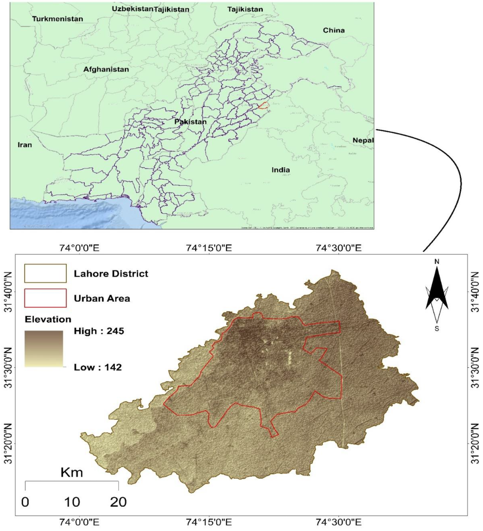
2. Study Area
3. Data and Methodology
3.1. Indicators Selection
3.2. Data Acquisition
3.3. Long Short-Term Memory
3.4. Time-Series Forecasting Using LSTM
3.5. Model Validation
4. Results and Discussions
5. Conclusions
5.1. Limitations
5.2. Implications and Future Research
Author Contributions
Funding
Institutional Review Board Statement
Informed Consent Statement
Data Availability Statement
Acknowledgments
Conflicts of Interest
References
- Sharifi, A.; Mahdipour, H.; Moradi, E.; Tariq, A. Agricultural Field Extraction with Deep Learning Algorithm and Satellite Imagery. J. Indian Soc. Remote Sens. 2022, 50, 417–423. [Google Scholar] [CrossRef]
- Bera, D.; Das Chatterjee, N.; Mumtaz, F.; Dinda, S.; Ghosh, S.; Zhao, N.; Bera, S.; Tariq, A. Integrated Influencing Mechanism of Potential Drivers on Seasonal Variability of LST in Kolkata Municipal Corporation, India. Land 2022, 11, 1461. [Google Scholar] [CrossRef]
- Ullah, I.; Aslam, B.; Shah, S.H.I.A.; Tariq, A.; Qin, S.; Majeed, M.; Havenith, H.-B. An Integrated Approach of Machine Learning, Remote Sensing, and GIS Data for the Landslide Susceptibility Mapping. Land 2022, 11, 1265. [Google Scholar] [CrossRef]
- Fu, C.; Cheng, L.; Qin, S.; Tariq, A.; Liu, P.; Zou, K.; Chang, L. Timely Plastic-Mulched Cropland Extraction Method from Complex Mixed Surfaces in Arid Regions. Remote Sens. 2022, 14, 4051. [Google Scholar] [CrossRef]
- Haq, S.M.; Tariq, A.; Li, Q.; Yaqoob, U.; Majeed, M.; Hassan, M.; Fatima, S.; Kumar, M.; Bussmann, R.W.; Moazzam, M.F.U.; et al. Influence of Edaphic Properties in Determining Forest Community Patterns of the Zabarwan Mountain Range in the Kashmir Himalayas. Forests 2022, 13, 1214. [Google Scholar] [CrossRef]
- Majeed, M.; Lu, L.; Haq, S.M.; Waheed, M.; Sahito, H.A.; Fatima, S.; Aziz, R.; Bussmann, R.W.; Tariq, A.; Ullah, I.; et al. Spatiotemporal Distribution Patterns of Climbers along an Abiotic Gradient in Jhelum District, Punjab, Pakistan. Forests 2022, 13, 1244. [Google Scholar] [CrossRef]
- Tariq, A.; Riaz, I.; Ahmad, Z. Land surface temperature relation with normalized satellite indices for the estimation of spatio-temporal trends in temperature among various land use land cover classes of an arid Potohar region using Landsat data. Environ. Earth Sci. 2020, 79, 40. [Google Scholar] [CrossRef]
- Tariq, A.; Shu, H. CA-Markov chain analysis of seasonal land surface temperature and land use landcover change using optical multi-temporal satellite data of Faisalabad, Pakistan. Remote Sens. 2020, 12, 3402. [Google Scholar] [CrossRef]
- Siddiqui, S.; Ali Safi, M.W.; Rehman, N.U.; Tariq, A. Impact of Climate Change on Land use/Land cover of Chakwal District. Int. J. Econ. Environ. Geol. 2020, 11, 65–68. [Google Scholar] [CrossRef]
- Tariq, A.; Shu, H.; Li, Q.; Altan, O.; Khan, M.R.; Baqa, M.F.; Lu, L. Quantitative Analysis of Forest Fires in Southeastern Australia Using SAR Data. Remote Sens. 2021, 13, 2386. [Google Scholar] [CrossRef]
- Majeed, M.; Tariq, A.; Anwar, M.M.; Khan, A.M.; Arshad, F.; Mumtaz, F.; Farhan, M.; Zhang, L.; Zafar, A.; Aziz, M.; et al. Monitoring of land use–Land cover change and potential causal factors of climate change in Jhelum district, Punjab, Pakistan, through GIS and multi-temporal satellite data. Land 2021, 10, 1026. [Google Scholar] [CrossRef]
- Mumtaz, F.; Arshad, A.; Mirchi, A.; Tariq, A.; Dilawar, A.; Hussain, S.; Shi, S.; Noor, R.; Noor, R.; Daccache, A.; et al. Impacts of reduced deposition of atmospheric nitrogen on coastal marine eco-system during substantial shift in human activities in the twenty-first century. Geomat. Nat. Hazards Risk 2021, 12, 2023–2047. [Google Scholar] [CrossRef]
- Waqas, H.; Lu, L.; Tariq, A.; Li, Q.; Baqa, M.F.; Xing, J.; Sajjad, A. Flash flood susceptibility assessment and zonation using an integrating analytic hierarchy process and frequency ratio model for the chitral district, khyber pakhtunkhwa, pakistan. Water 2021, 13, 1650. [Google Scholar] [CrossRef]
- Tariq, A.; Shu, H.; Siddiqui, S.; Mousa, B.G.; Munir, I.; Nasri, A.; Waqas, H.; Lu, L.; Baqa, M.F. Forest fire monitoring using spatial-statistical and Geo-spatial analysis of factors determining forest fire in Margalla Hills, Islamabad, Pakistan. Geomat. Nat. Hazards Risk 2021, 12, 1212–1233. [Google Scholar] [CrossRef]
- Hamza, S.; Khan, I.; Lu, L.; Liu, H.; Burke, F.; Nawaz-ul-Huda, S.; Baqa, M.F.; Tariq, A. The Relationship between Neighborhood Characteristics and Homicide in Karachi, Pakistan. Sustainability 2021, 13, 5520. [Google Scholar] [CrossRef]
- Tariq, A.; Shu, H.; Kuriqi, A.; Siddiqui, S.; Gagnon, A.S.; Lu, L.; Linh, N.T.T.; Pham, Q.B. Characterization of the 2014 Indus River Flood Using Hydraulic Simulations and Satellite Images. Remote Sens. 2021, 13, 2053. [Google Scholar] [CrossRef]
- Felegari, S.; Sharifi, A.; Moravej, K.; Amin, M.; Golchin, A.; Muzirafuti, A.; Tariq, A.; Zhao, N. Integration of Sentinel 1 and Sentinel 2 Satellite Images for Crop Mapping. Appl. Sci. 2021, 11, 10104. [Google Scholar] [CrossRef]
- Baqa, M.F.; Chen, F.; Lu, L.; Qureshi, S.; Tariq, A.; Wang, S.; Jing, L.; Hamza, S.; Li, Q. Monitoring and modeling the patterns and trends of urban growth using urban sprawl matrix and CA-Markov model: A case study of Karachi, Pakistan. Land 2021, 10, 700. [Google Scholar] [CrossRef]
- Hu, P.; Sharifi, A.; Tahir, M.N.; Tariq, A.; Zhang, L.; Mumtaz, F.; Shah, S.H.I.A. Evaluation of vegetation indices and phenological metrics using time-series modis data for monitoring vegetation change in Punjab, Pakistan. Water 2021, 13, 2550. [Google Scholar] [CrossRef]
- Tariq, A.; Yan, J.; Gagnon, A.S.; Riaz Khan, M.; Mumtaz, F. Mapping of cropland, cropping patterns and crop types by combining optical remote sensing images with decision tree classifier and random forest. Geo-spatial Inf. Sci. 2022, 1–19. [Google Scholar] [CrossRef]
- Tariq, A.; Mumtaz, F.; Zeng, X.; Baloch, M.Y.J.; Moazzam, M.F.U. Spatio-temporal variation of seasonal heat islands mapping of Pakistan during 2000–2019, using day-time and night-time land surface temperatures MODIS and meteorological stations data. Remote Sens. Appl. Soc. Environ. 2022, 27, 100779. [Google Scholar] [CrossRef]
- Schwarz, N.; Lautenbach, S.; Seppelt, R. Exploring indicators for quantifying surface urban heat islands of European cities with MODIS land surface temperatures. Remote Sens. Environ. 2011, 115, 3175–3186. [Google Scholar] [CrossRef]
- Qiao, Z.; Tian, G.; Xiao, L. Diurnal and seasonal impacts of urbanization on the urban thermal environment: A case study of Beijing using MODIS data. ISPRS J. Photogramm. Remote Sens. 2013, 85, 93–101. [Google Scholar] [CrossRef]
- Imran, M.; Mehmood, A. Analysis and mapping of present and future drivers of local urban climate using remote sensing: A case of Lahore, Pakistan. Arab. J. Geosci. 2020, 13, 278. [Google Scholar] [CrossRef]
- Shirazi, S.A.; Kazmi, J.H. Analysis of socio-environmental impacts of the loss of urban trees and vegetation in Lahore, Pakistan: A review of public perception. Ecol. Processes 2016, 5, 5. [Google Scholar] [CrossRef]
- Levermore, G.; Parkinson, J.; Lee, K.; Laycock, P.; Lindley, S. The increasing trend of the urban heat island intensity. Urban Climate 2018, 24, 360–368. [Google Scholar] [CrossRef]
- Debbage, N.; Shepherd, J.M. The urban heat island effect and city contiguity. Comput. Environ. Urban Syst. 2015, 54, 181–194. [Google Scholar] [CrossRef]
- Mathew, A.; Sreekumar, S.; Khandelwal, S.; Kaul, N.; Kumar, R. Prediction of surface temperatures for the assessment of urban heat island effect over Ahmedabad city using linear time series model. Energy Build. 2016, 128, 605–616. [Google Scholar] [CrossRef]
- Mathew, A.; Sreekumar, S.; Khandelwal, S.; Kumar, R. Prediction of land surface temperatures for surface urban heat island assessment over Chandigarh city using support vector regression model. Sol. Energy 2019, 186, 404–415. [Google Scholar] [CrossRef]
- Gobakis, K.; Kolokotsa, D.; Synnefa, A.; Saliari, M.; Giannopoulou, K.; Santamouris, M. Development of a model for urban heat island prediction using neural network techniques. Sustain. Cities Soc. 2011, 1, 104–115. [Google Scholar] [CrossRef]
- Lee, Y.Y.; Kim, J.T.; Yun, G.Y. The neural network predictive model for heat island intensity in Seoul. Energy Build. 2016, 110, 353–361. [Google Scholar] [CrossRef]
- Kolokotroni, M.; Davies, M.; Croxford, B.; Bhuiyan, S.; Mavrogianni, A. A validated methodology for the prediction of heating and cooling energy demand for buildings within the Urban Heat Island: Case-study of London. Sol. Energy 2010, 84, 2246–2255. [Google Scholar] [CrossRef]
- Khalil, U.; Aslam, B.; Azam, U.; Khalid, H.M.D. Time Series Analysis of Land Surface Temperature and Drivers of Urban Heat Island Effect Based on Remotely Sensed Data to Develop a Prediction Model. Appl. Artif. Intell. 2021, 35, 1803–1828. [Google Scholar] [CrossRef]
- Yu, X.; Shi, S.; Xu, L.; Liu, Y.; Miao, Q.; Sun, M. A novel method for sea surface temperature prediction based on deep learning. Math. Probl. Eng. 2020, 2020, 1–9. [Google Scholar] [CrossRef]
- Zhao, R.; Yan, R.; Chen, Z.; Mao, K.; Wang, P.; Gao, R.X. Deep learning and its applications to machine health monitoring. Mech. Syst. Signal Processing 2019, 115, 213–237. [Google Scholar] [CrossRef]
- Chen, L.; Liu, X.; Zeng, C.; He, X.; Chen, F.; Zhu, B. Temperature Prediction of Seasonal Frozen Subgrades Based on CEEMDAN-LSTM Hybrid Model. Sensors 2022, 22, 5742. [Google Scholar] [CrossRef]
- Tsokov, S.; Lazarova, M.; Aleksieva-Petrova, A. A Hybrid Spatiotemporal Deep Model Based on CNN and LSTM for Air Pollution Prediction. Sustainability 2022, 14, 5104. [Google Scholar] [CrossRef]
- Zhang, J.; Zhu, Y.; Zhang, X.; Ye, M.; Yang, J. Developing a Long Short-Term Memory (LSTM) based model for predicting water table depth in agricultural areas. J. Hydrol. 2018, 561, 918–929. [Google Scholar] [CrossRef]
- Garg, S.; Jindal, H. Evaluation of time series forecasting models for estimation of PM2.5 levels in air. In Proceedings of the 2021 6th International Conference for Convergence in Technology (I2CT), Maharashtra, India, 2–4 April 2021; pp. 1–8. [Google Scholar]
- Rana, I.A.; Bhatti, S.S. Lahore, Pakistan–Urbanization challenges and opportunities. Cities 2018, 72, 348–355. [Google Scholar] [CrossRef]
- Liang, B.; Weng, Q. Assessing urban environmental quality change of Indianapolis, United States, by the remote sensing and GIS integration. IEEE J. Sel. Top. Appl. Earth Obs. Remote Sens. 2010, 4, 43–55. [Google Scholar] [CrossRef]
- Mackey, C.W.; Lee, X.; Smith, R.B. Remotely sensing the cooling effects of city scale efforts to reduce urban heat island. Build. Environ. 2012, 49, 348–358. [Google Scholar] [CrossRef]
- Deng, C.; Wu, C. Examining the impacts of urban biophysical compositions on surface urban heat island: A spectral unmixing and thermal mixing approach. Remote Sens. Environ. 2013, 131, 262–274. [Google Scholar] [CrossRef]
- Guo, G.; Wu, Z.; Xiao, R.; Chen, Y.; Liu, X.; Zhang, X. Impacts of urban biophysical composition on land surface temperature in urban heat island clusters. Landsc. Urban Plan. 2015, 135, 1–10. [Google Scholar] [CrossRef]
- Mathew, A.; Khandelwal, S.; Kaul, N. Investigating spatial and seasonal variations of urban heat island effect over Jaipur city and its relationship with vegetation, urbanization and elevation parameters. Sustain. Cities Soc. 2017, 35, 157–177. [Google Scholar] [CrossRef]
- Alshaikh, A.Y. Space applications for drought assessment in Wadi-Dama (West Tabouk), KSA. Egypt. J. Remote Sens. Space Sci. 2015, 18, S43–S53. [Google Scholar] [CrossRef]
- Zhang, K.; Wang, R.; Shen, C.; Da, L. Temporal and spatial characteristics of the urban heat island during rapid urbanization in Shanghai, China. Environ. Monit. Assess. 2010, 169, 101–112. [Google Scholar] [CrossRef]
- Lazzarini, M.; Marpu, P.R.; Ghedira, H. Temperature-land cover interactions: The inversion of urban heat island phenomenon in desert city areas. Remote Sens. Environ. 2013, 130, 136–152. [Google Scholar] [CrossRef]
- Mathew, A.; Khandelwal, S.; Kaul, N. Spatial and temporal variations of urban heat island effect and the effect of percentage impervious surface area and elevation on land surface temperature: Study of Chandigarh city, India. Sustain. Cities Soc. 2016, 26, 264–277. [Google Scholar] [CrossRef]
- Huete, A.; Justice, C.; Van Leeuwen, W. MODIS vegetation index (MOD13). In Algorithm Theoretical Basis Document; University of Arizona: Tucson, AZ, USA, 1999; Version 3. [Google Scholar]
- Birhane, E.; Ashfare, H.; Fenta, A.A.; Hishe, H.; Gebremedhin, M.A.; Solomon, N. Land use land cover changes along topographic gradients in Hugumburda national forest priority area, Northern Ethiopia. Remote Sens. Appl. Soc. Environ. 2019, 13, 61–68. [Google Scholar] [CrossRef]
- Zhao, X.; Pu, J.; Wang, X.; Chen, J.; Yang, L.E.; Gu, Z. Land-use spatio-temporal change and its driving factors in an artificial forest area in Southwest China. Sustainability 2018, 10, 4066. [Google Scholar] [CrossRef]
- Imhoff, M.L.; Zhang, P.; Wolfe, R.E.; Bounoua, L. Remote sensing of the urban heat island effect across biomes in the continental USA. Remote Sens. Environ. 2010, 114, 504–513. [Google Scholar] [CrossRef]
- Zhang, Y.; Odeh, I.O.; Han, C. Bi-temporal characterization of land surface temperature in relation to impervious surface area, NDVI and NDBI, using a sub-pixel image analysis. Int. J. Appl. Earth Obs. Geoinf. 2009, 11, 256–264. [Google Scholar] [CrossRef]
- Hochreiter, S.; Schmidhuber, J. Long short-term memory. Neural Comput. 1997, 9, 1735–1780. [Google Scholar] [CrossRef] [PubMed]
- Gers, F.A.; Schmidhuber, J.; Cummins, F. Learning to forget: Continual prediction with LSTM. Neural Comput. 2000, 12, 2451–2471. [Google Scholar] [CrossRef]
- Chung, J.; Gulcehre, C.; Cho, K.; Bengio, Y. Empirical evaluation of gated recurrent neural networks on sequence modeling. arXiv 2014, arXiv:1412.3555. [Google Scholar] [CrossRef]
- Gers, F.A.; Schraudolph, N.N.; Schmidhuber, J. Learning precise timing with LSTM recurrent networks. J. Mach. Learn. Res. 2002, 3, 115–143. [Google Scholar]
- Graves, A.; Mohamed, A.-R.; Hinton, G. Speech recognition with deep recurrent neural networks. In Proceedings of the 2013 IEEE International Conference on Acoustics, Speech and Signal Processing, Vancouver, BC, Canada, 26–31 May 2013; pp. 6645–6649. [Google Scholar]
- Graves, A. Long short-term memory. In Supervised Sequence Labelling with Recurrent Neural Networks; Springer: Berlin/Heidelberg, Germany, 2012; pp. 37–45. [Google Scholar]
- Sak, H.; Senior, A.W.; Beaufays, F. Long short-term memory recurrent neural network architectures for large scale acoustic modeling. In Proceedings of the INTERSPEECH 2014, 15th Annual Conference of the International Speech Communication Association, Singapore, 14–18 September 2014. [Google Scholar]
- Wheatcroft, E. Interpreting the skill score form of forecast performance metrics. Int. J. Forecast. 2019, 35, 573–579. [Google Scholar] [CrossRef]
- Li, Y.-Y.; Zhang, H.; Kainz, W. Monitoring patterns of urban heat islands of the fast-growing Shanghai metropolis, China: Using time-series of Landsat TM/ETM+ data. Int. J. Appl. Earth Obs. Geoinf. 2012, 19, 127–138. [Google Scholar] [CrossRef]
- Tiangco, M.; Lagmay, A.; Argete, J. ASTER-based study of the night-time urban heat island effect in Metro Manila. International J. Remote Sens. 2008, 29, 2799–2818. [Google Scholar] [CrossRef]
- Mathew, A.; Chaudhary, R.; Gupta, N.; Khandelwal, S.; Kaul, N. Study of urban heat island effect on Ahmedabad City and its relationship with urbanization and vegetation parameters. Int. J. Comput. Math. Sci. 2015, 4, 126–135. [Google Scholar]
- Pal, S.; Ziaul, S. Detection of land use and land cover change and land surface temperature in English Bazar urban centre. Egypt. J. Remote Sens. Space Sci. 2017, 20, 125–145. [Google Scholar] [CrossRef]
- Zhang, H.; Qi, Z.-F.; Ye, X.-Y.; Cai, Y.-B.; Ma, W.-C.; Chen, M.-N. Analysis of land use/land cover change, population shift, and their effects on spatiotemporal patterns of urban heat islands in metropolitan Shanghai, China. Appl. Geogr. 2013, 44, 121–133. [Google Scholar] [CrossRef]
- Tariq, A.; Siddiqui, S.; Sharifi, A.; Hassan, S.; Ahmad, I. Impact of spatio—Temporal land surface temperature on cropping pattern and land use and land cover changes using satellite imagery, Hafizabad District, Punjab, Province of Pakistan. Arab. J. Geosci. 2022, 15, 1045. [Google Scholar] [CrossRef]
- Le, X.-H.; Ho, H.V.; Lee, G.; Jung, S. Application of long short-term memory (LSTM) neural network for flood forecasting. Water 2019, 11, 1387. [Google Scholar] [CrossRef]
- Liu, Y.; Li, D.; Wan, S.; Wang, F.; Dou, W.; Xu, X.; Li, S.; Ma, R.; Qi, L. A long short-term memory-based model for greenhouse climate prediction. Int. J. Intell. Syst. 2022, 37, 135–151. [Google Scholar] [CrossRef]


| Remote Sensing Product | Short Name | Sensor | Platform | Temporal Resolution | Spatial Resolution (m) |
|---|---|---|---|---|---|
| Land Surface Temperature and Emissivity | MYD11A2 | MODIS | Aqua | 8 Day | 926.626 |
| Vegetation Indices | MYD13A2 | MODIS | Aqua | 16 Day | 926.626 |
| Land Cover Type | MCD12Q1 | MODIS | Combined Aqua and Tera | Yearly | 463.3 |
| Global Digital Elevation Model | ASTGTM | ASTER | Terra | _ | 24.8 |
| Days No. | Type | Maximum | Minimum | Mean | Standard Deviation |
|---|---|---|---|---|---|
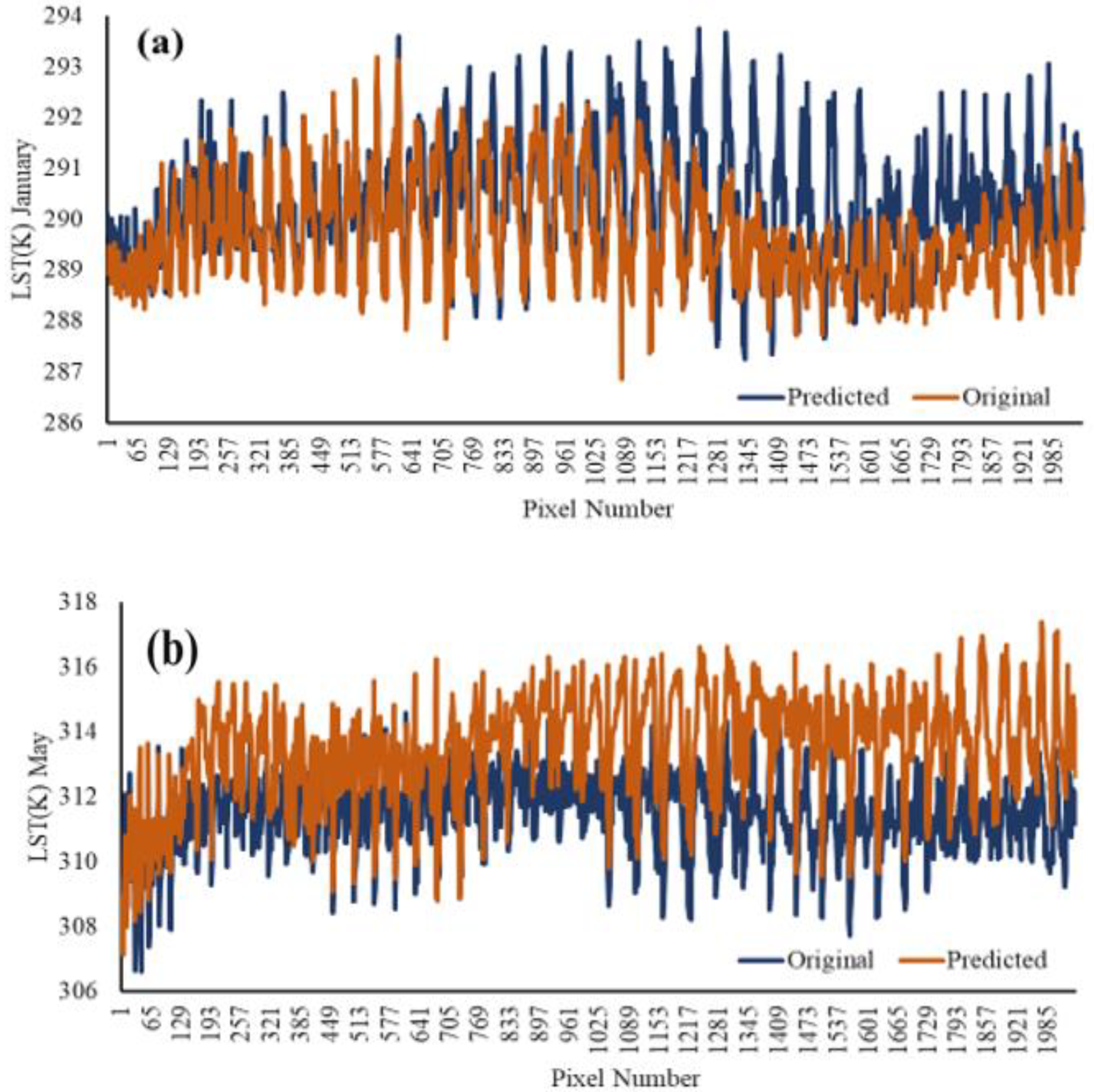
| 009–016 | Actual | 293.18 | 286.86 | 290.02 | 1.427 |
| Predicted | 293.51 | 288.94 | 291.22 | 1.348 | |
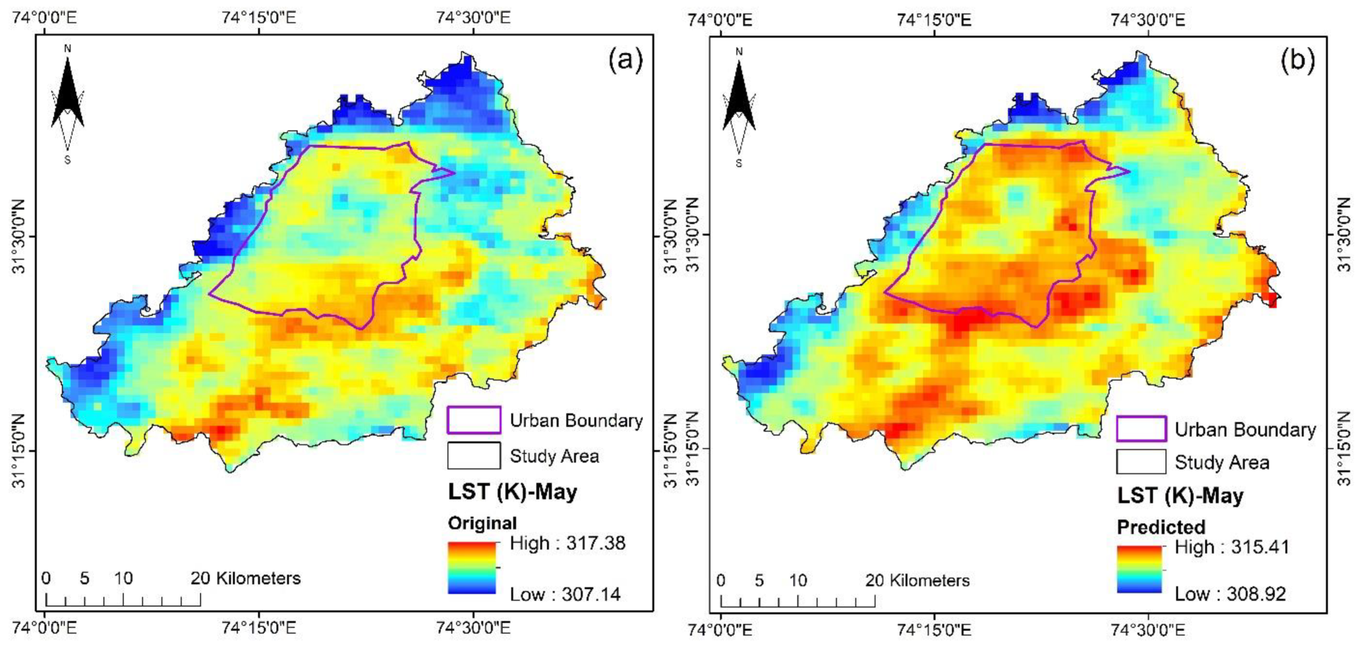
| 137–144 | Actual | 317.38 | 307.14 | 312.26 | 1.452 |
| Predicted | 315.41 | 308.92 | 312.16 | 1.416 |
| Model | Measures | January (009–016) | May (137–144) |
|---|---|---|---|
| MAE (K) | 0.27 | 0.27 | |
| LSTM (Forecasted) | MAPE (%) | 0.12 | 0.14 |
| MSE R2 | 0.242 0.95 | 0.253 0.94 | |
| ANN (Referred) | MSE | 0.264 | 0.296 |
| R2 | 0.93 | 0.93 |
| Time Period | Between −3.0 to −4.0 K | Between −2.0 to −3.0 K | Between −1.0 to −2.0 K | Between −1.0 to 0.0 K | Between 0.0 to 0.5 K |
|---|---|---|---|---|---|
| January (009–016) | 204 (5%) | 449 (11%) | 1551 (38%) | 1755 (43%) | 122 (3%) |
| Between −2.0 to −2.5 K | Between −1.0 to −2.0 K | Between −1.0 to 0.0 K | Between 0.0 to 1.0 K | Between 1.0 to 2.5 K | |
| May (137–144) | 286 (7%) | 122 (3%) | 1020 (25%) | 1551 (38%) | 1102 (27%) |
| Time Period | Between −5.0 to −3.0 K | Between −3.0 to −1.0 K | Between −1.0 to 0.0 K | Between 0.0 to 1.0 K | Between 1.0 to 0.2 K |
|---|---|---|---|---|---|
| January (009–016) | 219 (5%) | 543 (13%) | 1461 (36%) | 1583 (39%) | 275 (7%) |
| Between −2.0 to −1.0 K | Between −1.0 to 0.0 K | Between 0.0 to 2.0 K | Between 2.0 to 3.0 K | Between 3.0 to 5.0 K | |
| May (137–144) | 687 (17%) | 623 (15%) | 892 (22%) | 1243 (30%) | 636 (16%) |
| Model | Days No. | Skill Metric | Skill Score |
|---|---|---|---|
| LSTM | 9 | 0.474 | 0.426 |
| 73 | 0.684 | 0.228 | |
| ANN | 9 | 0.412 | 0.365 |
| 73 | 0.625 | 0.185 |
Publisher’s Note: MDPI stays neutral with regard to jurisdictional claims in published maps and institutional affiliations. |
© 2022 by the authors. Licensee MDPI, Basel, Switzerland. This article is an open access article distributed under the terms and conditions of the Creative Commons Attribution (CC BY) license (https://creativecommons.org/licenses/by/4.0/).
Share and Cite
Khalil, U.; Azam, U.; Aslam, B.; Ullah, I.; Tariq, A.; Li, Q.; Lu, L. Developing a Spatiotemporal Model to Forecast Land Surface Temperature: A Way Forward for Better Town Planning. Sustainability 2022, 14, 11873. https://doi.org/10.3390/su141911873
Khalil U, Azam U, Aslam B, Ullah I, Tariq A, Li Q, Lu L. Developing a Spatiotemporal Model to Forecast Land Surface Temperature: A Way Forward for Better Town Planning. Sustainability. 2022; 14(19):11873. https://doi.org/10.3390/su141911873
Chicago/Turabian StyleKhalil, Umer, Umar Azam, Bilal Aslam, Israr Ullah, Aqil Tariq, Qingting Li, and Linlin Lu. 2022. "Developing a Spatiotemporal Model to Forecast Land Surface Temperature: A Way Forward for Better Town Planning" Sustainability 14, no. 19: 11873. https://doi.org/10.3390/su141911873
APA StyleKhalil, U., Azam, U., Aslam, B., Ullah, I., Tariq, A., Li, Q., & Lu, L. (2022). Developing a Spatiotemporal Model to Forecast Land Surface Temperature: A Way Forward for Better Town Planning. Sustainability, 14(19), 11873. https://doi.org/10.3390/su141911873