Article

Study on Vehicle–Road Interaction for Autonomous Driving

1
School of Civil Engineering, Tsinghua University, Beijing 100084, China
2
School of Transportation Science and Engineering, Harbin Institute of Technology, Harbin 150090, China
3
College of Transportation and Logistics Engineering, Xinjiang Agricultural University, Urumqi 830052, China
*
Author to whom correspondence should be addressed.
Sustainability 2022, 14(18), 11693; https://doi.org/10.3390/su141811693
Submission received: 30 July 2022 / Revised: 13 September 2022 / Accepted: 14 September 2022 / Published: 17 September 2022
(This article belongs to the Special Issue Progress and Challenge of Sustainable Transportation Infrastructure)

Abstract

:
Autonomous vehicles (AVs) are becoming increasingly popular, and this can potentially affect road performance. Road performance also influences driving comfort and safety for AVs. In this study, the influence of changes in traffic volume and wheel track distribution caused by AVs on the rutting distress of asphalt pavement was investigated through finite element simulations. A vehicle-mounted three-dimensional laser profiler was used to obtain pavement roughness and texture information. The vehicle vibration acceleration was obtained through vehicle dynamics simulations, and the skid resistance indexes of 20 rutting specimens were collected. The results showed that an increase in traffic volume caused by the increasing AV traffic accelerated the occurrence of rutting distress; however, the uniform distribution of vehicles at both ends of the transverse direction could prolong the maintenance life of flexible and semi-rigid pavements by 0.041 and 0.530 years, respectively. According to Carsim and Trucksim vehicle simulations and multiple linear regression fitting, the relationship models of three factors, namely speed, road roughness, and comfort, showed high fitting accuracies; however, there were some differences among the models. Among the texture indexes, the arithmetic mean’s height (Ra) had the greatest influence on the tire–road friction coefficient; Ra greatly influenced the safe driving of AVs. The findings of this study were used to present a speed control strategy for AVs based on the roughness and texture index for ensuring comfort and safety during automatic driving.

1. Introduction

Autonomous vehicle (AV) technology would provide great convenience to the elderly or disabled [1,2], and reduce traffic accidents and air pollution [3]. Fleets of share AVs may become cheaper than other modes in relative terms [4]. Therefore, the public has had a high acceptance rate of AVs in recent years [5]. Many countries have taken a step further by testing their AVs on public roads [6]. However, the interaction between AVs and roads seems to only have received a limited amount of attention to the best of our knowledge. Some studies have concluded that the control mode and impact of AVs considerably change traffic flow compared with human-driving vehicles (HVs), which would affect the structure and performance of asphalt pavements [7,8]. On the other hand, the speed control and braking strategies of AVs rarely consider the influence of the roughness and texture characteristics of pavements on driving safety and comfort [9,10]. Given the rapid growth in vehicle automation technology, there is a pressing need to uncover the impact of AVs on the pavement and formulate the control strategy of AVs based on pavement performance.
For AVs’ influence on the service performance of asphalt pavements, Chen et al. [11] proposed that a reduction in vehicle lateral can accelerate the occurrence of pavement rutting distress; they indicated that a lateral uniform distribution of AVs can reduce rutting damage. Farah et al. [12] reported that by ensuring the precise positioning of AVs, road width is flexible and can be reduced in the future; however, this may aggravate the occurrence of pavement distress. Zhou et al. [13] found that the standard deviation of lateral displacement of AVs was at least three times smaller than that of HVs and that AVs can decrease the fatigue life of pavements by 20% and increase rut depth by 13%. However, these studies have only considered changes in the lateral positioning mode of AVs and have not considered the impact of traffic flow changes caused by the presence of AVs on pavement performance. The research shows that an increase in AVs’ penetration rate leads to a shortening of following distance and an increase in traffic speed [14,15], thus improving the traffic volume and traffic flow efficiency. Variations in traffic volume and in vehicle speed change the load repetitions on pavements, which leads to a change in road performance. Therefore, to obtain more accurate insights, the impact of changes in traffic flow and the lateral distribution caused by the presence of AVs on pavement performance should be comprehensively considered.
Vehicle speed control plays an important role in the comfort and safety of AVs. To ensure passenger comfort, Mohajer et al. [16] generated a comfortable path profile according to a road curvature, and a directional path tracking unit optimized the AV’s trajectory using a controller and a speed regulator. CHOI et al. [17] proposed a coupled controller based on game theory, which realizes AVs’ speed planning in regards to vehicle dynamics and considers acceleration changes when the vehicle changes direction to ensure passenger comfort. Nguyen et al. [18] developed a control framework based on a fuzzy model to deal with the time-varying characteristics of vehicle speed. In terms of improving driving safety, Fu et al. [19] proposed an AV braking strategy based on deep reinforcement learning, and adopted a behavior criticism algorithm to solve the autonomous braking problem. Yuan et al. [20] proposed a new compact active braking system for AVs, which was based on adaptive gain-scheduling proportional differential controller and logic threshold control. Gounis et al. [21] designed a layered automatic emergency braking system based on safety distance. Emergency braking can meet the requirements of the safety distance threshold under the condition of a constant tire friction coefficient. However, the above studies put forward speed control strategies from the perspective of a vehicle speed controller or braking system, not addressing the fact that pavement performance is the fundamental source of vehicle vibration and braking force. Roughness and texture characteristics have a great impact on passenger comfort and braking safety [9,22]. Therefore, vehicle speed control based on pavement performance is the key to improving the driving comfort and safety of AVs.
The emergence of the Geographic Information System (GIS) and Vehicular Ad-Hoc Network (VANET) [23] has made it possible for AVs to have control based on pavement performance. The pavement performance collected by the pavement detection equipment can be shared through the VANET technology [24,25], which provides technical support for the AVs to optimize their driving behavior according to the pavement performance. However, in terms of pavement performance data collection technology, the accelerometer [26] is affected by the vehicle speed and suspension system in the process of pavement roughness data collection, resulting in data distortion. Moreover, the method of using optical sensors to collect pavement roughness and texture [27,28] is greatly affected by lighting conditions. Thus, using hand-held close range camera technology to collect pavement texture information [22] cannot meet requirements for the rapid investigation of a large-area road network. Therefore, it is crucial to ensure the accurate investigation and rapid update of road information, which can enable AVs to obtain road information in real time and formulate appropriate speed control strategies.
Given the above problems, this paper aims to study the influence of AVs’ popularization on pavement performance and to formulate speed control strategies for AVs based on pavement performance. For this purpose, flexible and semi-rigid pavements were simulated using finite element simulations firstly, and the coupling effect of changes in traffic volume and wheel track distribution caused by increased AV traffic on rut depth was analyzed. Then, a vehicle-mounted high-precision three-dimensional (3D) laser profiler was used to collect data about pavement roughness and texture, and the relationships between roughness and comfort, the texture index and skid resistance were investigated. An AV control strategy based on roughness and texture was proposed. The discussion of the results and concluding remarks are presented in the final section.

2. Test Materials and Method

2.1. Test Materials

To analyze the relationship between pavement texture and skid resistance, rutting specimens with different gradations were prepared. The technical indexes of the 70# matrix asphalt, the technical indexes of the aggregate, and the grading curves of different rutting specimens are presented in Table 1 and Table 2, and Figure 1, respectively. It can be seen from Table 1 that the test results of all indexes of the 70# matrix asphalt used in this research meet the specification requirements, so the 70# matrix asphalt is sufficient.

2.2. Test Method

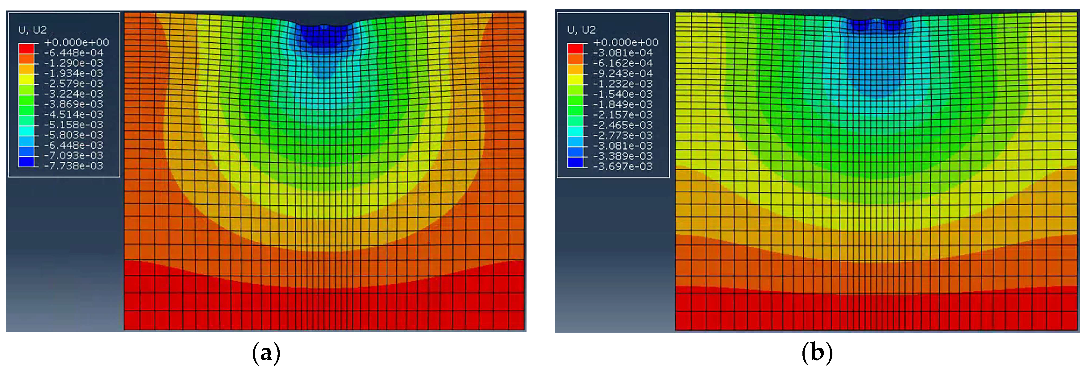
2.2.1. Simulation Calculation of Pavement Rutting

(1)
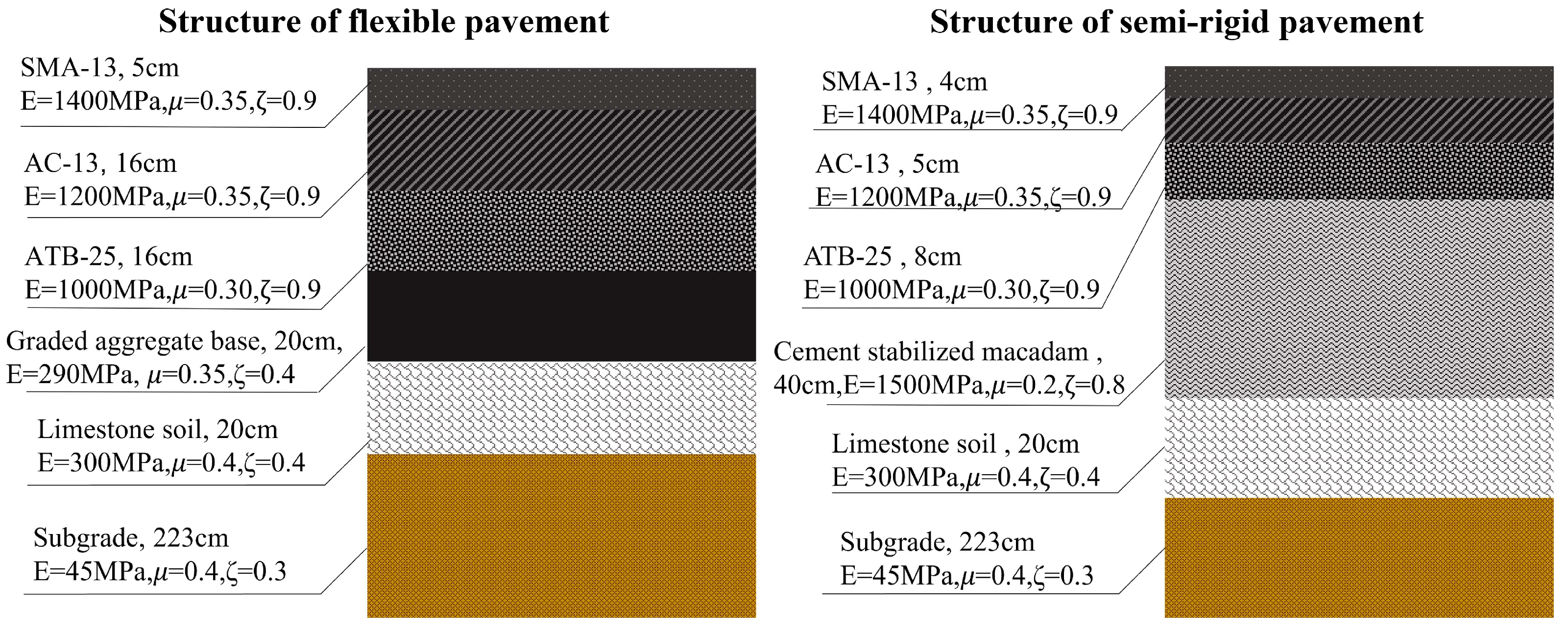
Finite element model of the pavement structure
According to Chinese specification JTG D50-2017 concerning typical pavement structures in China, two-dimensional finite element models of flexible and semi-rigid pavement structures were established in this study. The pavement structure parameters are presented in Figure 2. The width of finite element models of flexible pavement and semi-rigid pavement was 3.75 m and the thickness was 3 m. The model mesh element type was CPE8R, and the mesh of the wheel on-board action area was locally refined. The boundary conditions of the model were set as no horizontal displacement in the lateral direction and no vertical displacement at the bottom, and the contact between layers was complete. The load conditions are shown in Table 3.
In both the pavement models, the horizontal width and depth were 3.75 and 3 m, respectively. The grid of the load action area was locally refined. For the model, the following boundary conditions were used: there was no lateral horizontal displacement, there was no vertical displacement at the bottom, and the layers of the pavement were in complete contact. Asphalt pavements have viscoelastic–plastic characteristics under the action of load and temperature [30]; rutting is mainly caused by creep deformation. Therefore, the Drucker–Prager model was adopted, as shown in Equation (1).
ε ˙ c r = ( A q n [ ( m + 1 ) ε ¯ c r ] m ) 1 m + 1
where ε ˙ c r is the uniaxial equivalent creep strain rate, ε ¯ c r is the uniaxial equivalent creep strain, q is the eccentric stress, and model parameters A, n, and m, as well as the thermal property parameters of the asphalt pavement temperature field were taken according to the relevant literature [31].
(2)
Load parameters
According to Chinese specification JTG D50-2017, 100 kN was selected as the design standard axle load. The specific parameters are presented in Table 3. The cumulative action time of the load was calculated using Equation (2).
t = 0.36 N P n w p B v
where t is the cumulative action time of the wheel load (s), N is the number of wheel load repetitions, nw is the number of axles (4), v is the vehicle speed (80 km/h), P is the standard load, p is the tire grounding pressure (0.7 Mpa) and B is the rectangular width of single-wheel grounding.

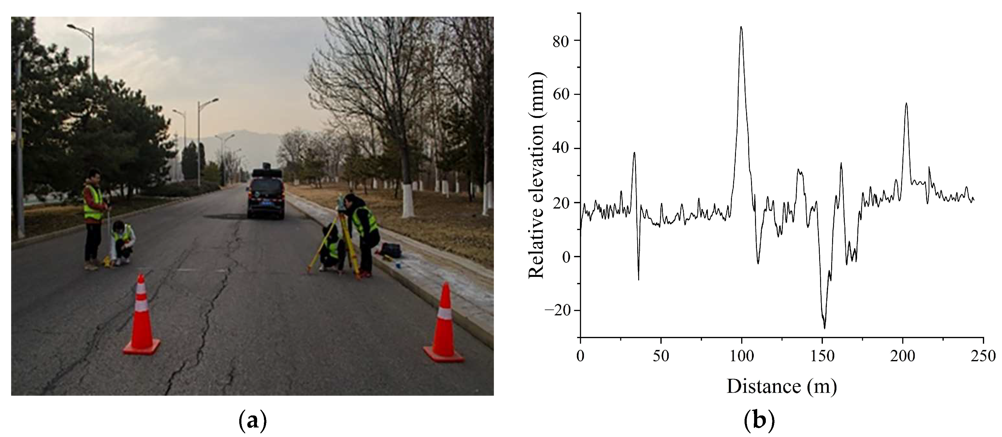
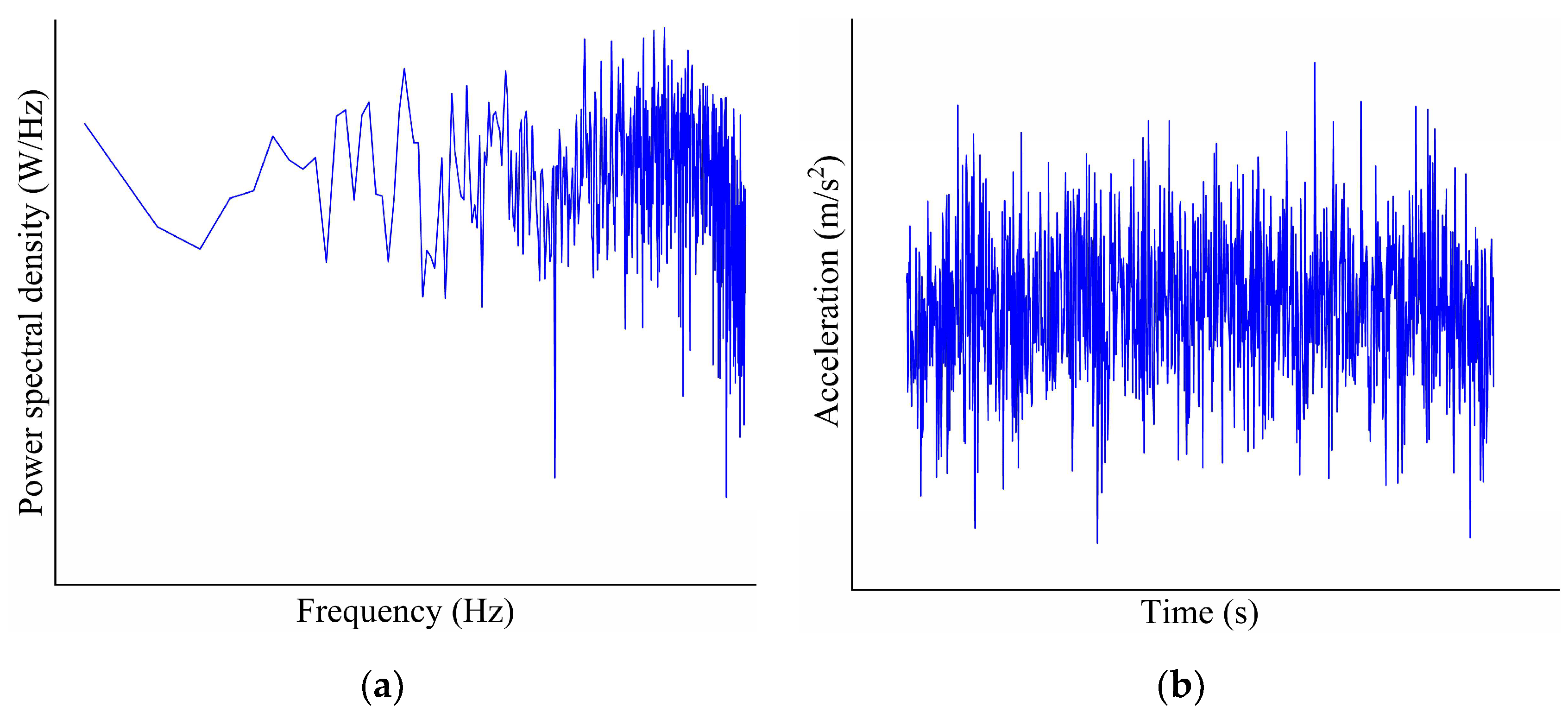
2.2.2. Acquisition of Road Roughness and Vehicle Vibration Acceleration

To collect roughness data accurately, a 3D laser profiler (Figure 3b) was used; it was developed according to laser triangulation to collect the longitudinal contour elevation data of the road surface of the vehicle track (Figure 3c). The obtained longitudinal contour elevation was input into a quarter of the golden car model after algorithm filtering to calculate the international roughness index (IRI).
By moving the reference algorithm in the elevation direction, vibration errors were effectively eliminated without installing an accelerometer; thus, roughness could be accurately measured in any driving state [32], thereby effectively overcoming the inherent limitations of the accelerometer in the inertial profiler. Different locations on Wenyang road, Haidian district, Beijing, were selected for testing. Figure 4 shows the test scenario and the relative elevation data of the road section.
To collect vibration acceleration data during vehicle driving, whole vehicle models of Carsim and Trucksim software were used to establish a virtual sample vehicle (Figure 5). Default parameters of the model were used for the vehicle body, tires, suspension, transmission device, and aerodynamism. In the software, the road centerline method was used to input the road contour elevation values collected by employing the detection vehicle into the model to reproduce the uneven state of the road space. Finally, the acceleration data of the seat in the left and right, front and rear, and up and down directions was collected.

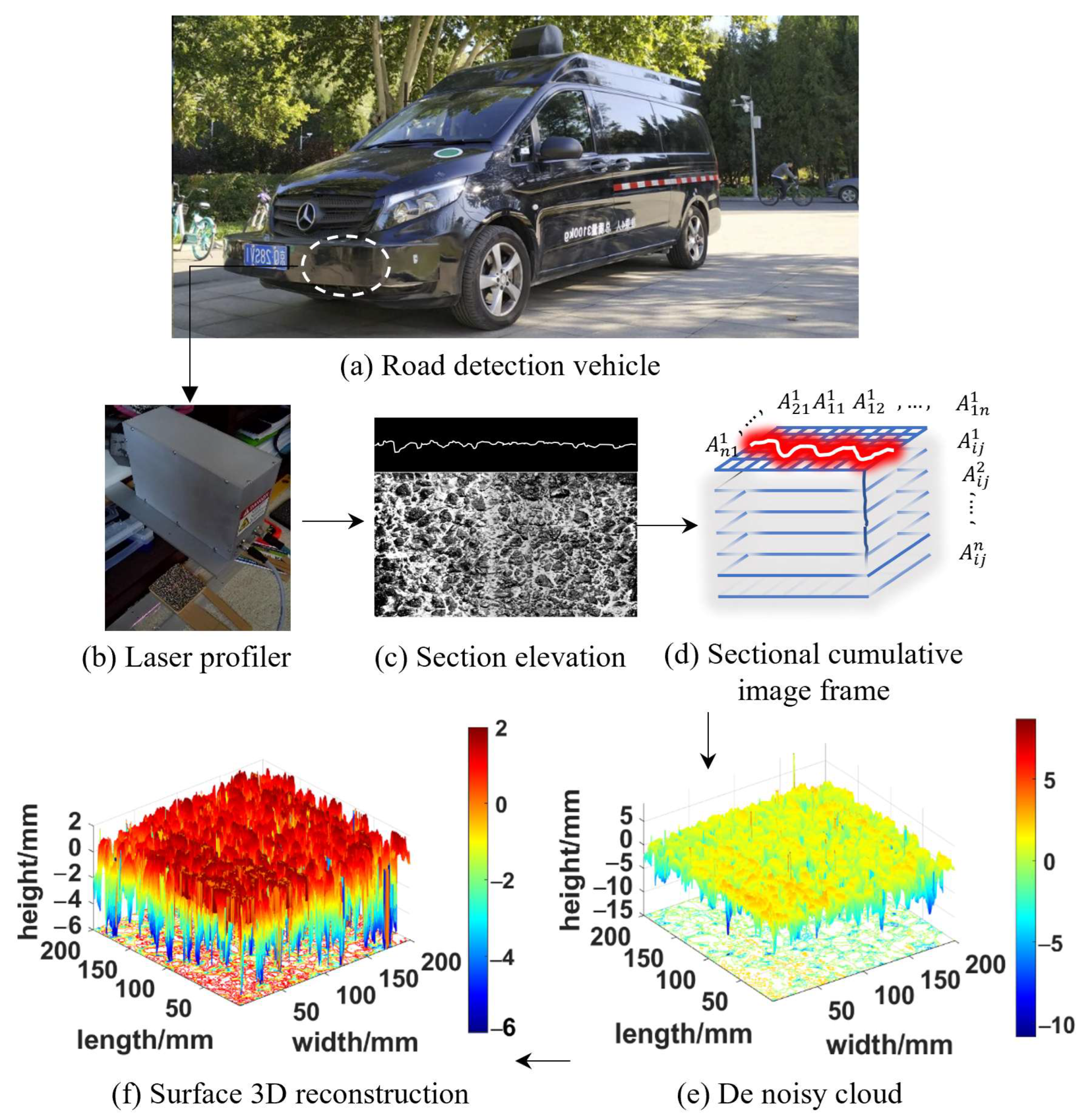
2.2.3. Acquisition of Pavement Texture and Skid Resistance

To collect pavement texture data, the 3D laser profiler was arranged horizontally; accumulated image frames of the rutting specimen section were collected at 60 km/h. The accumulated image frames were used for the 3D reverse reconstruction of the pavement by using the built-in algorithm (Figure 3e). The vertical accuracy reached 0.01 mm, which is better than the accuracy (1 mm) of the contemporary full-lane fast laser profiler [33]. Moreover, the micro and macro texture boundaries were high (0.05 mm) [32]. Some of the texture indexes used in the study included the Ra, Rq, MTD and MPD (see Table A1 in Appendix A for the definition of the indexes); these were calculated from the 3D texture data [32]. Concerning Chinese standard JTG E60–2008, the sliding resistance of rutting specimens was evaluated using a pendulum friction instrument.

3. Results and Discussion

3.1. Influence of AVs on Rutting

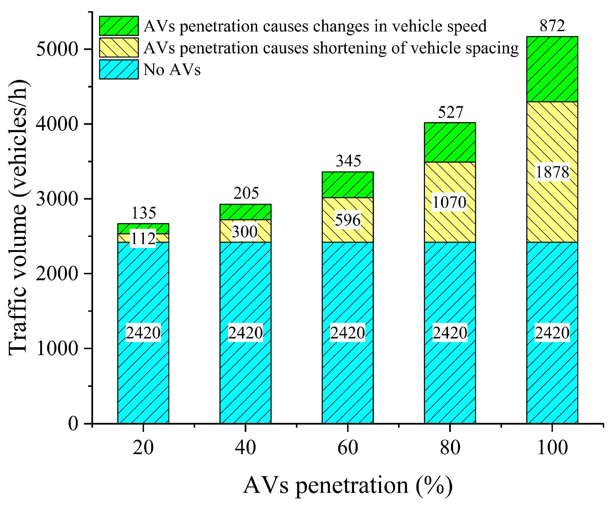
3.1.1. Influence of AVs Popularization on Traffic Volume

Traffic volume is determined by traffic density and vehicle speed. The traffic density is the reciprocal of the lane length occupied by vehicles [34]. The traffic volume of HVs (Ch) can be calculated using Equation (3). Since AVs have the features including information sharing, an accurate perception of the surrounding environment and rapid decision-making control functions, they can greatly reduce the vehicle braking reaction time. Therefore, compared with HVs, AVs can follow the vehicle at a smaller temporal distance (time gap) (Taa) [8]. In a traffic flow composed of fully AVs, the traffic volume Ca is calculated by Equation (4). The ratio of the two traffic volume calculation equations is shown in Equation (5). It can be seen that when the vehicle speed and the vehicle length are the same, the change in traffic volume is determined by the time gap.
In mixed traffic flow, since HVs have no communication function, when an HV follows AV, the time gap between the HV and AV is equal to the time gap between the HVs (Thh), which can be expressed as Thx. When an AV follows an HV, the AV and HV cannot realize the information interaction, which degenerates into the adaptive cruise control in which the AV uses sensors to judge the state of the vehicle ahead [35]; the time gap between the AV and HV (Tah) is less than Thx but greater than Taa. The modified traffic volume (Cm) calculation equation is shown in Equation (6) [8].
C h = v v T h h + L
C a = v v T a a + L
C h C a = v T a a + L v T h h + L
C m = v g 2 v T a a + g ( 1 g ) v T a h + ( 1 g ) v T h x + L p k w
where Thh is the time gap to the preceding vehicle (s), L is the vehicle length (m), v is the vehicle speed (m/s), g is AVs penetration (%), Taa is the time gap between AVs (0.5 s), Thx is the time gap between HVs and the front vehicle (1.15 s). Tah is the time gap between AVs and front HVs (0.9 s), Lpkw is the length of the lane occupied by the vehicle (7.5 m), including the length of the vehicle and the safe distance between the vehicle and the vehicle in front. The parameters in Equations (3)–(6) are taken according to reference [8].
The research shows that with the increase in AVs’ penetration rate, the traffic speed can be significantly increased, and vehicles can quickly pass through the traffic bottleneck area to reduce traffic congestion [14,36]. When the AVs’ penetration rate reaches 100%, the traffic speed can be increased by 45–72% [37,38]. At AV penetration rates of 20%, 40%, 60%, 80% and 100%, the vehicle speed is increased by 27%, 38%, 57%, 67% and 72%, respectively [38]. Considering the changes in the time gap and traffic speed caused by the popularization of AVs, we calculated the traffic volume under five kinds of AV penetration rates according to Equation (6), and the results are shown in Figure 6.
Figure 6 shows that as the vehicle speed and driving distance changed due to higher AV traffic, the traffic volume increased; at a high AV penetration rate ( 40%), the resulting change in driving distance was the main factor that increased traffic volume. At the AV penetration rates of 20%, 40%, 60%, 80% and 100%, the traffic volume increased by 10%, 21%, 39%, 67% and 114%, respectively.

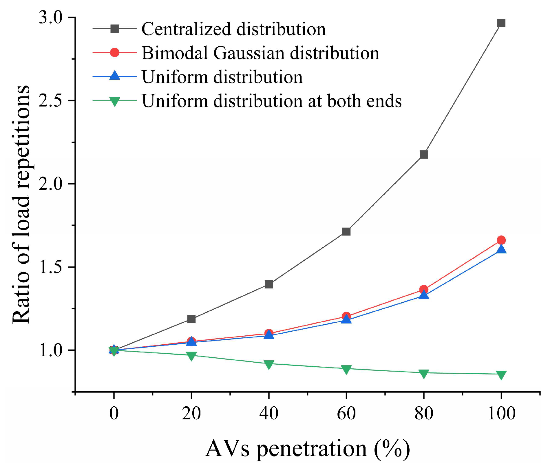
3.1.2. Influence of AVs Popularization on Load Repetitions

With continuous advances in algorithms and control systems, the lateral control strategy of AVs is becoming increasingly robust. In the future, the programmed distribution of the wheels’ lateral trajectory can be realized; then, road performance will be mainly influenced by heavy-duty vehicles. Chen et al. [11] considered a truck model and proposed that the lateral distribution of the wheel trajectory of HVs is the normal distribution. In the future, AVs may appear centrally distributed, with uniform distribution at both ends, including bimodal Gaussian normal distribution and uniform distribution. The wheel trace distribution equation and schematic diagram are shown in Table 4.
The synthetic transverse distribution function at different AV penetration rates can be calculated using Equation (7).
F i j ( x ) = w j * f ( x ) + ( 1 w j ) * g i ( x )
where wj is the proportion of HVs; i—0,1,2,3 correspond to the four lateral distribution modes of the wheel tracks in AVs; f(x) is the load frequency curve of HVs; and gi(x) is the load frequency of AVs. A double wheel with a width = 466 mm was considered as the main wheel trace belt [39], and the effective load frequency within the track belt was calculated; that is, the load frequency curve was integrated within the range of x = [607, 1073] to obtain the probability density, and it was the ratio of the load repetitions in the wheel track belt to the total load repetitions in the section [7,40].
The influence of changes in vehicle load repetitions caused by changes in traffic volume on the pavement structure was not considered. Herein, the coupling effect of AV distribution mode and traffic volume change was considered, and the ratio of the number of load repetitions in the wheel track belt under different AV penetration rates to the number of load repetitions in the wheel track belt without AVs was calculated, as shown in Figure 7.
Figure 7 shows that by considering the changes in traffic volume and speed caused by higher traffic of AVs, the wheel track mode with uniform distribution at both ends can effectively reduce the load repetitions in the wheel track belt of vehicles in case of high-AV traffic. In Figure 7, the ratio of the load repetitions in the wheel track belt with a bimodal Gaussian distribution and uniform distribution under different AV penetration rates shows a similar trend, because in the tire load action interval x = [607, 1073], the ratios of the load repetitions in the wheel track with a bimodal Gaussian distribution and uniform distribution to the total load repetitions in the section were 56% and 54%, respectively, which was close. After the two-wheel track lateral distribution functions were substituted into Equation (7), the proportion of the load repetitions in the wheel track belt to the total load repetitions of the section under different AV penetration rates obtained by integration were close. This results in a similar trend in the ratio of the load repetitions in the wheel track belt of the two-wheel track distributions to the load repetitions in the wheel track belt without AVs under different AV penetration rates.

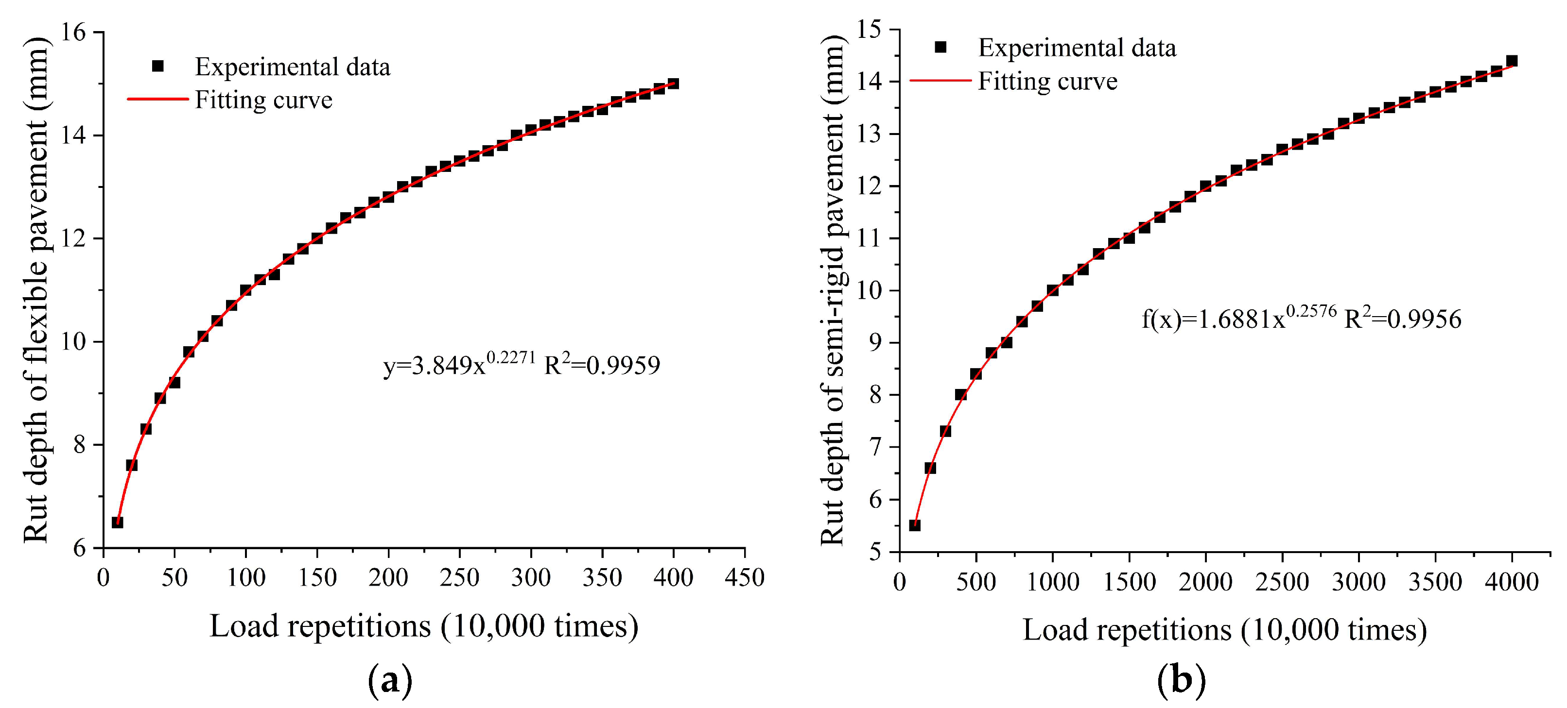
3.1.3. Influence of AVs Popularization on Rutting

According to the finite element model established in Section 2.1, the rutting depth under different load repetitions was calculated and regressed to obtain the relationship between rutting depth and load repetitions. The relationship between rutting depth and standard axle load repetitions of the two pavements is shown in Figure 8.
Figure 8 shows that the rut depth increased with an increase in load repetitions. At the same load repetitions, the rut depth of the semi-rigid pavement was less than that of the flexible pavement, indicating the better rutting resistance of the semi-rigid pavement. A cloud diagram of rut distress in the flexible and semi-rigid pavements under twenty thousand load repetitions is shown in Figure 9.
When the wheel track distribution change was not considered, the increase in traffic volume caused by higher AV traffic aggravated the rutting distress of the pavement. For flexible and semi-rigid pavements, when the load repetitions reached 3.9907 and 48.1742 million times, respectively, the pavement rutting depth reached the maintenance rut depth (15 mm). Considering the lateral distribution of the wheel tracks of AVs, for the four lateral distribution modes of wheel tracks, under the condition of 100% AV penetration, the pavement maintenance period was calculated according to the relationship between road rutting and load repetitions (Figure 8). The results are shown in Figure 10.
At the AV penetration rate of 0, the maintenance periods of the flexible and semi-rigid pavements were 0.264 and 3.150 years, respectively. As shown in Figure 10, high AV traffic increased traffic volume; however, the uniform distribution of vehicles at both ends of the horizontal direction could reduce the occurrence of rutting distress and extend the maintenance life of flexible and semi-rigid pavements by 0.041 and 0.530 years, respectively. In Figure 10, there was a large difference between the maintenance period of uniform distribution at both ends and that of uniform distribution. This is because when the AVs’ penetration rate was 100%, the ratios of the number of load repetitions in the track belt under uniform distribution and uniform distribution at both ends to the number of load repetitions in the track belt without AVs were 1.60 and 0.86, respectively. The number of load repetitions in the wheel track belt under uniform distribution was 1.86 times that of uniform distribution at both ends. The above phenomenon indicates that to achieve the same number of load repetitions in the wheel track belt and the same rutting depth in the wheel track belt, the traffic volume of a single lane with a uniform distribution at both ends of the wheel track needs to be 1.86 times that of the uniform distribution [41], resulting in a large difference in maintenance period under the two distribution modes.

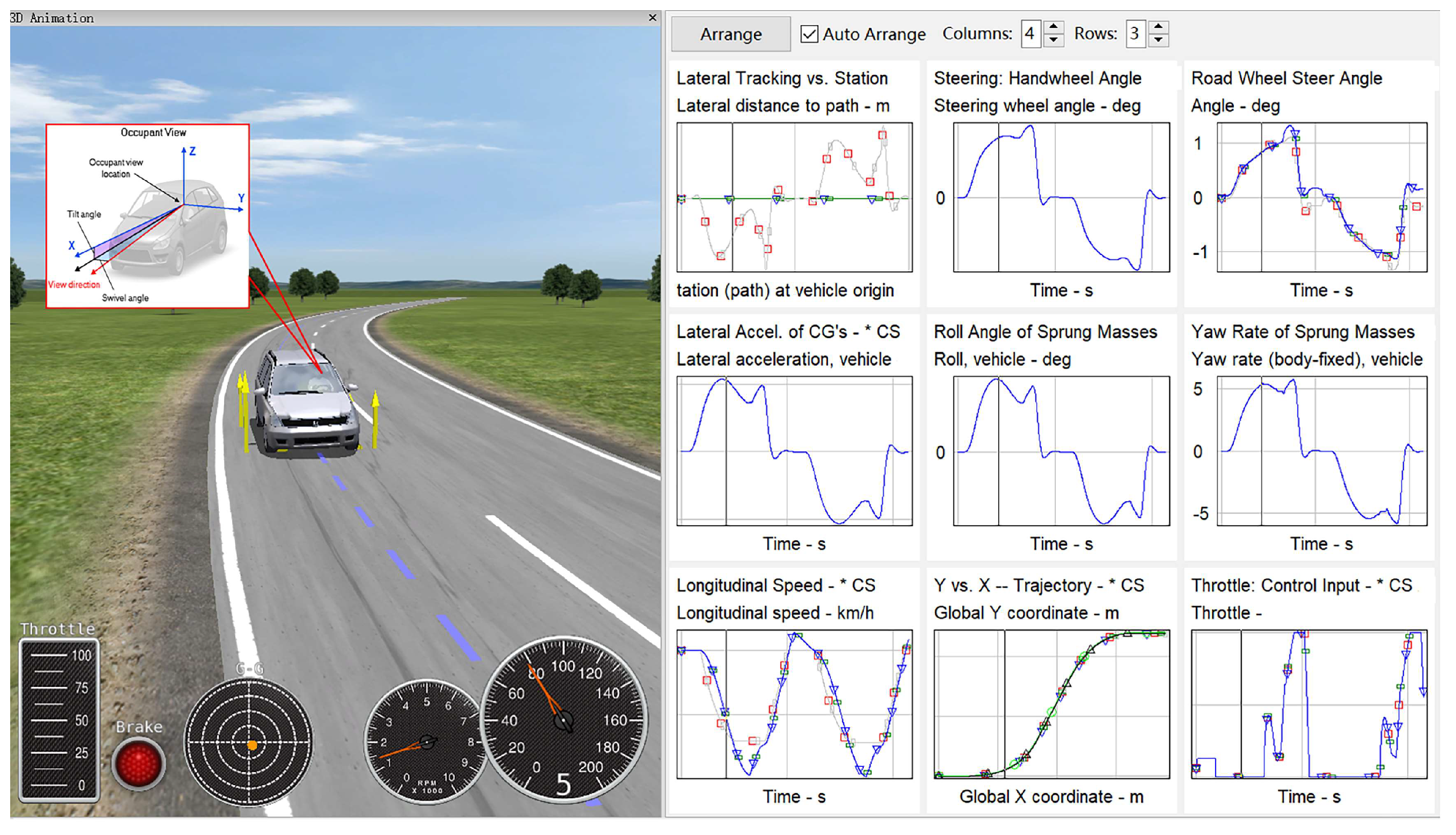
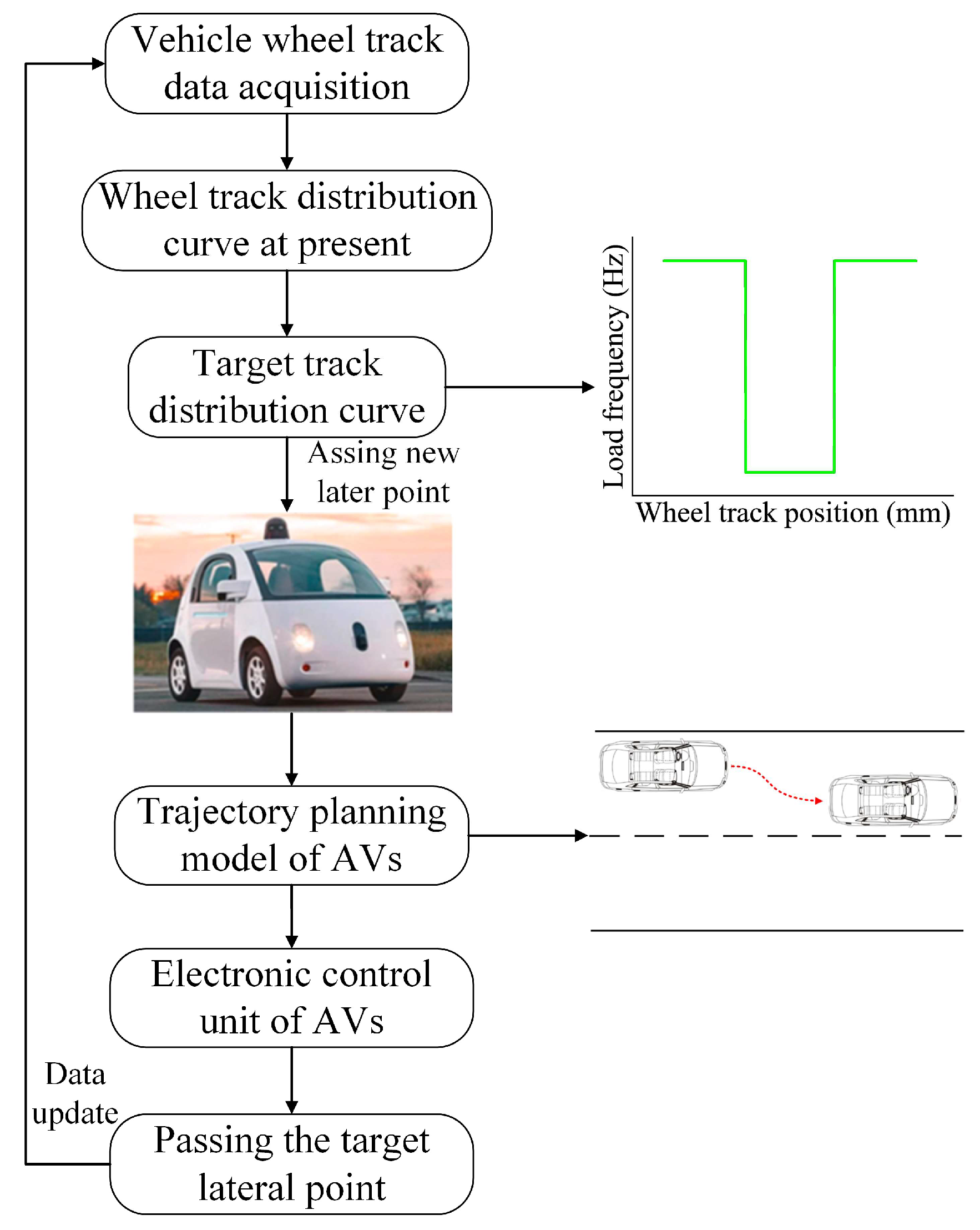
3.1.4. The Framework of Lateral Control on AVs

Note that this section mainly focuses on the influence of traffic volume and wheel track distribution changes caused by AVs on rutting distress, for which the method to achieve the target wheel track lateral distribution curve is briefly introduced as follows.
Video detection and the Internet of Things are used to collect the driving track of vehicles on the road ahead [42], and the current road wheel track distribution curve is obtained. The AVs obtain the current wheel track distribution curve through V2I technology. The current lateral position of AVs is known, and a new lateral position on the future lane is assigned to AVs according to the parameters, such as the target track distribution curve and the lane width.
According to the trajectory planning model [43], the electronic control unit of AVs determines the route (distance and trajectory alignment) required for the trajectory change, and generates steering information; the steering motor realizes steering and reaches the designated lateral distribution point. After the current AV passes through the target lateral point, the wheel track distribution curve is updated to control the lateral position of the subsequent AVs. The AVs’ lateral distribution strategy is shown in Figure 11.

3.2. Influence of Road Performance on Driving Behavior of AVs

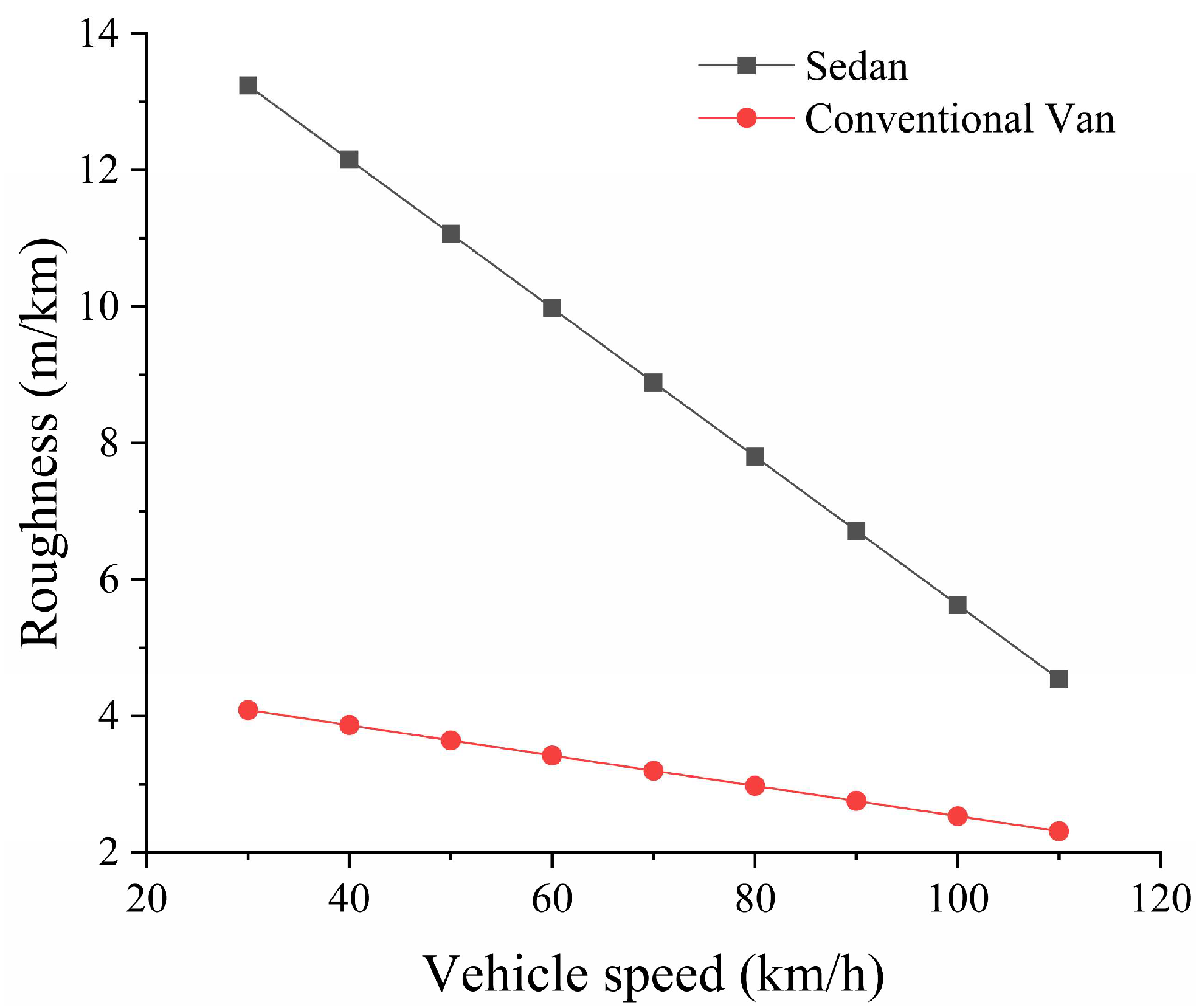
3.2.1. Relationship between Roughness and AVs Comfort

After obtaining the road roughness and vehicle vibration acceleration in Section 2.2.2, the total weighted root mean square acceleration method was used to evaluate comfort. Before calculating the root mean square value of total weighted acceleration, the root mean square value of uniaxial weighted acceleration was calculated. First, the acceleration self-power spectrum function, Ga(f), was obtained using the spectral analysis of the acceleration in each axis, and then, the one-way weighted root mean square value of acceleration, aw, was calculated through the direct integration of Ga(f) according to Equation (8).
a w = 0.5 80 w 2 ( f ) G a ( f ) d f
where f is frequency (Hz); w(f) is the frequency weighting function. For w(f) with different axes, see Equations (9) and (10) for the functional relationship.
w z ( f ) = { 0.5 ,   0.5 f < 2 f 4 ,   2 f < 4 1 ,   4 f < 12.5 12.5 f ,   12.5 f 80
w x ( f ) = w y ( f ) = { 1 ,   0.5 f < 2 2 f ,   2 f 80
The root mean square value of the total weighted acceleration was calculated using Equation (11).
a w 0 = ( 1.4 a w x ) 2 + ( 1.4 a w y ) 2 + ( a w z ) 2
where aw0 is the root mean square value of total weighted acceleration(m/s2); awx, awy and awz are the root mean square value of acceleration in the directions of the X-axis, Y-axis, and Z-axis, respectively (m/s2).
The acceleration data obtained in the vehicle dynamics experiment were discrete data that changed with time. To accurately express it using mathematical expressions, time-domain sequence data were first converted (Figure 12a) into frequency-domain sequence data (Figure 12b). In the calculation of the root mean square value of weighted acceleration, the power spectral density function of acceleration data was calculated according to Equation (12).
+ x 2 ( t ) d t = + | x ( f ) | 2 d f
where x(f) is the Fourier transform function of time-domain acceleration, t is time (s) and f is the frequency (Hz).
In the simulation software, different vehicle models were selected to drive on roads with different roughness at different speeds. The vibration acceleration of the vehicle was collected, and the root mean square of the weighted acceleration was calculated. Vibration acceleration, speed and roughness data were subject to multiple linear regressions by using SPSS software. A small sedan car and a conventional truck van were considered examples, and the relationships between acceleration, roughness and speed were represented using Equations (13) and (14).
a w = 0.046 I R I + 0.005 v 0.194 , R 2 = 0.961
a w = 0.135 I R I + 0.003 v 0.077 , R 2 = 0.917
When the goodness of fit R2 was close to 1, the fitting effect of the regression equation was considered good. The goodness of fit of the regression equation in Equations (13) and (14) was >0.9, indicating that the function expression was well fitted with the observed values. This value was selected as the critical value to determine passenger comfort in transit; the critical value of roughness based on passenger comfort was obtained for different models at different driving speeds. The results are shown in Figure 13. A greater roughness value implied a bumpier road.
As shown in Figure 12, the requirement for roughness increases with an increase in vehicle speed; therefore, AVs should actively reduce vehicle speed to ensure human comfort when the roughness of the road ahead is poor. At the same speed, the critical value of roughness required to meet the riding comfort of trucks was considerably smaller than that of cars, indicating that different speed control strategies can be specified for different AVs.

3.2.2. Pavement Texture and Safe Driving Behavior of AVs

(1)
Correlation analysis between pavement texture and skid resistance
Five groups of rutting specimens (20 pieces) with different grading were scanned using a 3D laser, and skid resistance was examined. The Pearson correlation method [44] was employed to calculate the correlation between multiple indicators. The results are shown in Figure 14. An SPSS was used to calculate the standardized influence coefficient of the macro texture index (β) on BPN. The results are shown in Figure 15.
As shown in Figure 13, among the macro texture indexes, only the Pearson coefficient between Ra and MPD is >0.8; the two indexes are strongly correlated. In terms of the correlation between the macro texture and BPN, the correlation between Ra and BPN was 0.928, which indicated a high correlation. The correlation between other macro texture indexes and BPN was <0.8, which showed a moderate correlation. The order of weight of each texture index on BPN value was Ra > Rq > MPD > MTD.
(2)
Skid resistance and driving safety of AVs
Considering the correlation and standardized weight influence coefficients, the detection value of Ra was used to predict the skid resistance of the pavements. The regression of BPN and Ra was calculated using Equation (15).
B P N = 29.269 R a + 40.942
The conversion relationship between pavement friction coefficient, μ , and BPN was given using Equation (16) [45].
μ = ( 110 B P N 1 3 ) 1
Finally, the conversion relationship between μ and Ra was obtained using Equation (17).
μ = 87.807 R a + 122.826 289.058 29.269 R a
After obtaining the texture index Ra of the pavement ahead, the AV calculated the road friction coefficient by using Equation (17), and thus, determined the expected braking acceleration to ensure safe driving.
During driving, excessive lateral offset distance is an important factor that may lead to road accidents. Therefore, the road texture data were calculated using Equation (15) to obtain the dynamic friction coefficient for different roads with the considered vehicles; the calculated dynamic friction coefficient was input into the Carsim vehicle simulation software for simulating the safe driving of AVs. The results are presented in Figure 15.
As shown in Figure 16, the offset distance difference of the AV model developed by Carsim can be accurate to the order of 0.0001 m, which is higher than the detection requirements of the centimeter level [46], with high accuracy. It can distinguish the lateral offset difference of AV to the scale of <1 mm, indicating that the model had high reliability. Different pavement initial states had good skid resistance; thus, the texture structure provided by the road surface to the tire–road contact was relatively good. Among the three gradation types, the texture structure provided by AC-13 to AVs for safe driving was more complete.

3.2.3. Speed Control Strategy of AVs Based on Pavement Performance

Based on the relationship between driving comfort of AVs and roughness, safety and road texture, this study introduced a hyperbolic tangent function of speed control, as shown in Equation (18) [47] and proposed a speed control strategy for AVs based on pavement performance. Acceleration and deceleration were symmetrical; therefore, only the speed adjustment strategy under deceleration was considered:
v f = ( b + ε ) tanh ( k ( t τ ) ) b + v 0
where vf is final speed (m/s), v0 is initial speed (m/s), b is half of the absolute speed difference between final speed and initial speed (m/s), t is time (s), k is the stability coefficient that determines the shape of the speed change, τ is the time constant [26,47], tanh is the hyperbolic tangent function, changing the value of k can adjust the speed of curve change, and the error is ε ( ε > 0 ) .
The acceleration produced during vehicle deceleration (ad) is calculated according to Equation (19).
a d = ( b + ε ) k [ 1 ( tanh ( k ( t τ ) ) ) 2 ]
The deceleration process was assumed to take place in the longitudinal direction, ignoring the lateral acceleration. In the influence of roughness on vehicle vibration, vertical acceleration had the most considerable influence. When decelerating, longitudinal acceleration was mainly considered; hence, the root mean square value of weighted acceleration (adv) was expressed using Equation (20).
a d v = ( ω v a v ) 2 + ( ω d a d ) 2
where ω v and ω d were the weights of road roughness and acceleration caused by vehicle deceleration, respectively; av is the vehicle vibration acceleration (m/s2).
The critical value of vibration acceleration for passenger comfort was a = 0.565 m/s2 [48]. Therefore, vehicle vibration acceleration was calculated using Equation (21), max | a d v | 0.565 m / s 2 :
a v = x I R I + y v + z
where IRI is the roughness of pavement ahead (m/km); v is the target speed of road ahead (m/s); and x, y and z are the equation constants of different models. The stability coefficient k calculated by ensuring that the acceleration does not exceed the passenger comfort limit during deceleration is expressed by k1 and calculated according to Equation (22):
k 1 0.319 ( ω v a v ) 2 ( b + ε ) ω d = 0.319 [ ω v ( x I R I + y v + z ) ] 2 ( b + ε ) ω d
Furthermore, the bumpiness limit for comfortable driving should also be considered. Bumps manifest as the rate of change of vehicle longitudinal acceleration [49]; studies have shown that vehicle bumps considerably influence comfort. Hubbard [50] reported that turbulence should not exceed 2.94 m/s3 to ensure passenger comfort, as shown in Equation (23). The stability coefficient k to ensure that the vehicle bumps do not exceed the passenger comfort limit is expressed by k2, which is calculated according to Equation (24).
4 9 ( b + ε ) k 2 2.94 m / s 3
k 2 2.57 b + ε
When an AV detects an obstacle in front and there is a need for emergency braking, it will not consider the driver’s reaction time; the resulting braking distance was calculated using Equation (21).
d = v 0 ( t a + t s 2 ) + v 0 2 2 g μ
where v0 is initial speed, ta is system response and commissioning time, ts is braking force growth time, and g is gravitational acceleration.
The acceleration provided by the ground friction force is μ g [51], and the maximum braking of the vehicle is obtained as Equation (26) by combining Equation (19).
a max = ( b + ε ) k = 2 g μ
The stability coefficient k calculated under the maximum braking acceleration is expressed by k3. By combining Equations (17) and (26), the relationship between k3 and Ra was obtained, as shown in Equation (27).
175.614 g R a + 245.652 g ( 289.058 29.269 R a ) ( b + ε ) = k 3
After determining the stability coefficient k, in combination with the speed change curve function shown in Equation (18), the deceleration time and distance can be calculated according to Equations (28) and (29), respectively.
t = a r tanh ( b b + ε ) a r tanh ( b b + ε ) k = 2 a r tanh ( b b + ε ) k
s = τ 0 τ f v d t = b + 2 ε 2 k ln [ tanh ( k ( t τ ) ) + 1 ] + ( v 0 + ε ) t | τ 0 τ f = 2 k ( v 0 + ε ) a r tanh ( b b + ε ) + b + 2 ε 2 k ln ( ε b + ε )
Thus, this paper presents a detailed speed control strategy for AVs, as shown in Figure 17.
AVs obtain the real-time roughness and texture information of the road ahead using sensing modules or V2I technology; these data are transmitted to the motion planning module and further processed in combination with the environmental information and vehicle status. According to the roughness of the road ahead, to ensure that the acceleration and bumps produced during the shifting process do not exceed the passenger comfort limit, the AV calculates the stability coefficients k1 and k2; based on the texture information, the AV calculates a stability coefficient k3 that provides the maximum braking acceleration. When the distance between the AV and vehicle (obstacle) in front is greater than the safe braking distance, only the passenger comfort is considered, and the minimum value of k1 and k2 is taken as the stability coefficient k of the target speed change curve; otherwise, k2 is taken as the stability coefficient k of the target speed change curve. Finally, the AV produces a new speed curve according to the updated k value to complete the speed control under the premise of ensuring the comfort and safety of passengers.

4. Conclusions

In this study, the vehicle–road interaction for AVs was investigated using finite element simulation, road detection vehicle data acquisition and vehicle dynamics simulation. The main findings are as follows.
(1)
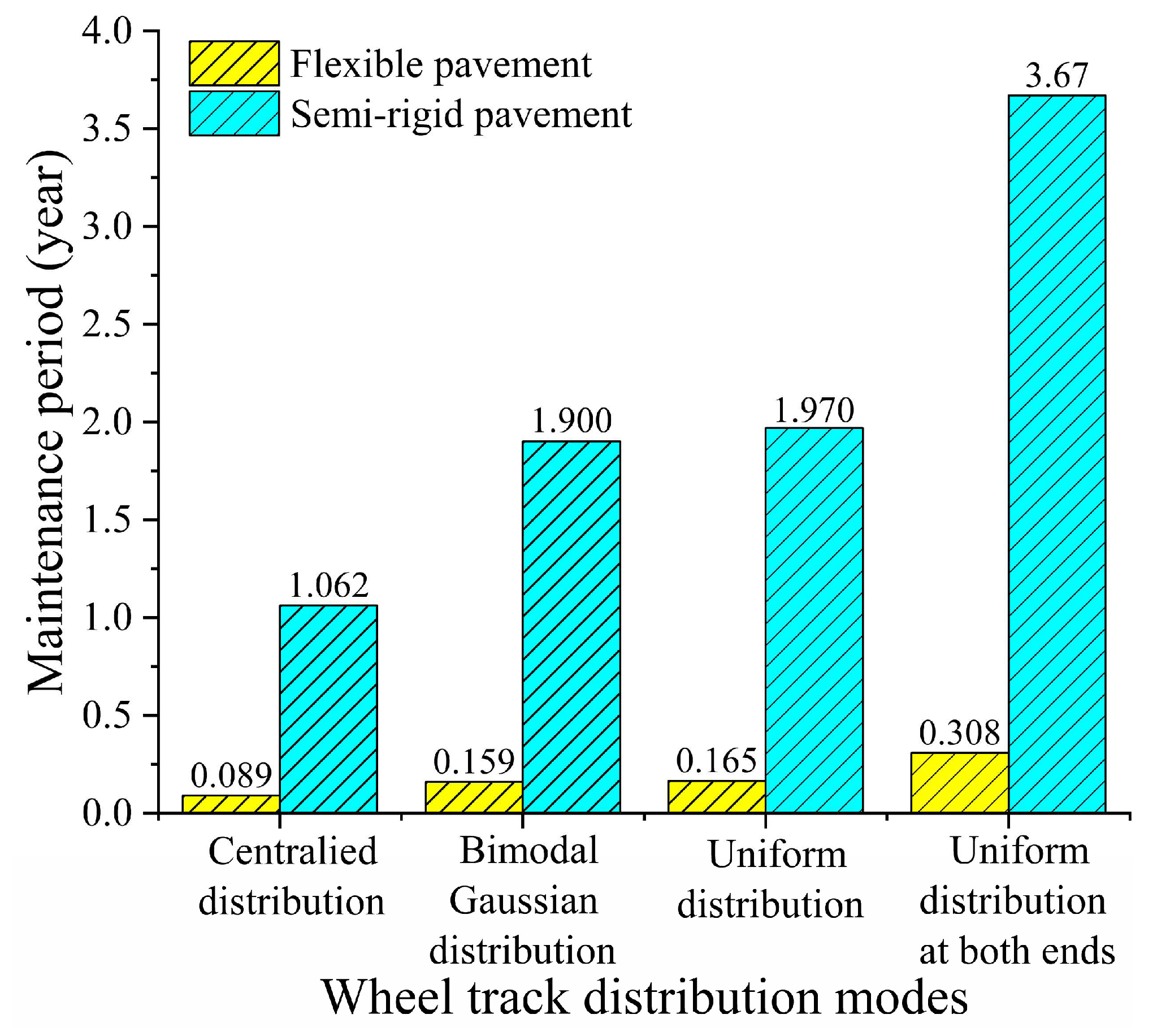
Considering the change in traffic volume caused by AVs, the semi-rigid pavement has a longer maintenance period than flexible pavement under various wheel track distribution modes. When the AVs’ penetration rate reaches 100%, only the uniform distribution at both ends can reduce the number of loads in the wheel track by 24.3%, and prolong the maintenance period of flexible pavement and semi-rigid pavement by 0.041 and 0.53 years, respectively.
(2)
There is a linear relationship between roughness and passenger comfort. The goodness of fit of the comfort prediction model based on roughness and vehicle speed is almost one. To ensure the comfort of passengers, the AVs should reduce the speed as the roughness becomes worse. Under the same road roughness, the critical value of vehicle speed to meet the comfort of truck passengers is significantly smaller than that of cars, which indicates that specific vehicle speed control strategies need to be formulated for different vehicle types.
(3)
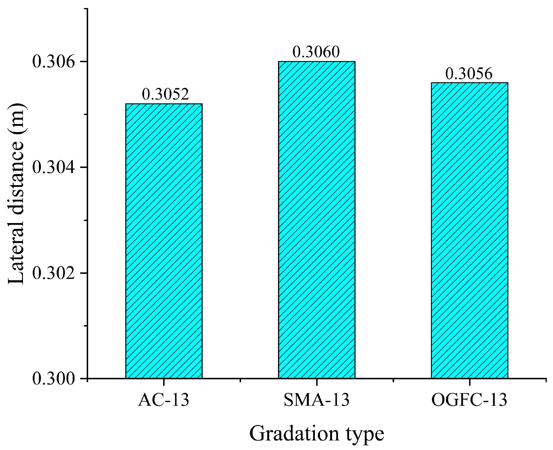
In the relationship between texture index and BPN, the correlation coefficient between Ra and BPN is 0.928, and the influence coefficient of Ra on BPN is 0.973, which is higher than other texture indexes. It proves the effectiveness of using Ra to predict the road friction coefficient. In the Carsim vehicle dynamic simulation, the texture structure provided by AC-13 to AVs for safe driving was more complete.
(4)
In the aspect of lateral control of AVs, this paper proposes that the lateral position of AVs can be assigned according to the current and target wheel track distribution curve, and trajectory planning can be carried out. However, the specific mode and effect of the lateral intervention of the wheel track of AVs need further research, and the feasibility and reliability of the lateral control should be evaluated.
(5)
In the speed control of AVs, the hyperbolic tangent speed function curve was introduced in this paper. Considering the influence of pavement performance on riding comfort and braking safety, the stability coefficient k of the speed curve was determined to realize the speed control of AVs. In the future, the difference between the speed control strategy of AVs and HVs can be studied in depth, and the influence of different vehicle types and different driving environments on the speed control strategy of AVs can be analyzed.

Author Contributions

Conceptualization, S.L. and R.G.; methodology, S.L. and Y.H.; software, S.L. and Y.H.; validation, R.G., S.L.; formal analysis, S.L. and L.X.; investigation, S.L. and L.X.; resources, S.L. and R.G.; data curation, S.L.; writing—original draft preparation, S.L.; writing—review and editing, S.L. and Y.H.; visualization, S.L. All authors have read and agreed to the published version of the manuscript.

Funding

This research received no external funding.

Institutional Review Board Statement

No applicable.

Informed Consent Statement

No applicable.

Data Availability Statement

The data presented in this study are available on request from the corresponding author. The data are not publicly available due to confidentiality promised to research participants.

Conflicts of Interest

The authors declare no conflict of interest.

Appendix A

The definitions of symbols in this paper are summarized, as shown in Table A1.
Table A1. Symbols and definitions.
SymbolsDefinitions
ε ˙ c r The uniaxial equivalent creep strain
ε ¯ c r The uniaxial equivalent creep strain
qEccentric stress
ACreep parameter
nCreep parameter
mCreep parameter
tTtime
NThe number of wheel load actions
nwThe number of axles
vVehicle speed
PStandard load
pTire grounding pressure
BThe rectangular width of single wheel grounding
ChTraffic volume of HVs
CaTraffic volume of AVs
CmTraffic volume of AVs and HVs mixed traffic flow
LVehicle length
gAVs penetration
ThhThe time gap to the preceding vehicle
TaaThe time gap between AVs and front HVs
ThxThe time gap between HVs and front vehicle
TahThe time gap between AVs and front HVs
LpkwThe length of lane occupied by vehicle
Fij(x)The synthetic transverse distribution function
wjThe proportion of HVs
f(x)Load frequency curve of HVs
gi(x)Load frequency of AVs
Ga(f)The acceleration self-power spectrum function
w(f)Frequency weighting function
wx(f)Frequency weighting function in x-axis direction
wy(f)Frequency weighting function in y-axis direction
wz(f)Frequency weighting function in Z-axis direction
fFrequency
awOne-way weighted root mean square value of acceleration
awxRoot mean square value of acceleration in X-axis
awyRoot mean square value of acceleration in y-axis
awzRoot mean square value of acceleration in z-axis
x(f)The Fourier transform function of time-domain acceleration
IRIInternational roughness index
BPNBritish pendulum number
MPDMean profile depth
MTDMean texture depth
RqRoot mean square deviation of the profile
RaAverage deviation of the contour arithmetic
μ Friction coefficient
vfFinal speed
v0Initial speed
bHalf of the absolute speed difference
ε Error
kStability coefficient that determines the shape of the speed change
k1Stability coefficient calculated by ensuring that the acceleration does not Exceed the passenger comfort limit during deceleration
k2Stability coefficient calculated by ensuring the vehicle bumps do not exceed the passenger comfort limit
k3Stability coefficient calculated under the maximum braking acceleration
τ Time constant
tanhHyperbolic tangent function
advRoot mean square value of weighted acceleration
avVehicle vibration acceleration
adAcceleration produced during vehicle deceleration
wwThe weights of road roughness
wdThe weights of acceleration caused by vehicle deceleration

References

  1. Sun, H.; Jing, P.; Zhao, M.; Chen, Y.; Zhan, F.; Shi, Y. Research on the Mode Choice Intention of the Elderly for Autonomous Vehicles Based on the Extended Ecological Model. Sustainability 2020, 12, 10661. [Google Scholar] [CrossRef]
  2. Miller, K.; Chng, S.; Cheah, L. Understanding acceptance of shared autonomous vehicles among people with different mobility and communication needs. Travel Behav. Soc. 2022, 29, 200–210. [Google Scholar] [CrossRef]
  3. Nuzzolo, A.; Persia, L.; Comi, A.; Polimeni, A. Shared Autonomous Electrical Vehicles and Urban Mobility: A Vision for Rome in 2035. In Conference on Sustainable Urban Mobility; Springer: Cham, Switzerland, 2019; pp. 772–779. [Google Scholar] [CrossRef]
  4. Bosch, P.M.; Becker, F.; Becker, H.; Axhausen, K.W. Cost-based analysis of autonomous mobility services. Transp. Policy 2018, 64, 16. [Google Scholar] [CrossRef]
  5. Becker, F.; Axhausen, K.W. Literature review on surveys investigating the acceptance of automated vehicles. Transportation 2017, 44, 1293–1306. [Google Scholar] [CrossRef]
  6. Abu Bakar, A.I.; Abas, M.A.; Said, M.F.M.; Azhar, T.A.T. Synthesis of Autonomous Vehicle Guideline for Public Road-Testing Sustainability. Sustainability 2022, 14, 1456. [Google Scholar] [CrossRef]
  7. Chen, F.; Balieu, R.; Kringos, N. Potential influences on long-term service performance of road infrastructure by automated vehicles. Transp. Res. Rec. J. Transp. Res. Board 2016, 2550, 72–79. [Google Scholar] [CrossRef]
  8. Friedrich, B. The effect of autonomous vehicles on traffic. In Autonomous Driving; Springer: Berlin, Germany, 2016; pp. 317–334. [Google Scholar] [CrossRef]
  9. Du, Y.; Chen, J.; Zhao, C.; Liu, C.; Liao, F.; Chan, C.-Y. Comfortable and energy-efficient speed control of autonomous vehicles on rough pavements using deep reinforcement learning. Transp. Res. Part C Emerg. Technol. 2021, 134, 103489. [Google Scholar] [CrossRef]
  10. Zheng, B. Research on Skid Resistance of Asphalt Pavement and Measurement Requirements for Autonomous Vehicle during Braking Process; Southeast University: Dhaka, Bangladesh, 2021. [Google Scholar]
  11. Chen, F.; Song, M.; Ma, X.; Zhu, X. Assess the impacts of different autonomous trucks’ lateral control modes on asphalt pavement performance. Transp. Res. Part C Emerg. Technol. 2019, 103, 12. [Google Scholar] [CrossRef]
  12. Farah, H.; Erkens, S.M.J.G.; Alkim, T.; van Arem, B. Infrastructure for Automated and Connected Driving: State of the Art and Future Research Directions. In Road Vehicle Automation 4; Springer: Berlin, Germany, 2018; pp. 187–197. [Google Scholar]
  13. Zhou, F.; Hu, S.; Chrysler, S.T.; Kim, Y.; Damnjanovic, I.; Talebpour, A.; Espejo, A. Optimization of Lateral Wandering of Automated Vehicles to Reduce Hydroplaning Potential and to Improve Pavement Life. Transp. Res. Rec. J. Transp. Res. Board 2019, 2673, 81–89. [Google Scholar] [CrossRef]
  14. Fagnant, D.J.; Kockelman, K. Preparing a nation for autonomous vehicles: Opportunities, barriers and policy recommendations. Transp. Res. Part A Policy Pract. 2015, 77, 167–181. [Google Scholar] [CrossRef]
  15. Deluka Tibljaš, A.; Giuffrè, T.; Surdonja, S.; Trubia, S. Introduction of Autonomous Vehicles: Roundabouts Design and Safety Performance Evaluation. Sustainability 2018, 10, 1060. [Google Scholar] [CrossRef]
  16. Mohajer, N.; Nahavandi, S.; Abdi, H.; Najdovski, Z. Enhancing Passenger Comfort in Autonomous Vehicles Through Vehicle Handling Analysis and Optimization. IEEE Intell. Transp. Syst. Mag. 2020, 13, 156–173. [Google Scholar] [CrossRef]
  17. Choi, Y.-M.; Park, J.-H. Game-Based Lateral and Longitudinal Coupling Control for Autonomous Vehicle Trajectory Tracking. IEEE Access 2021, 10, 31723–31731. [Google Scholar] [CrossRef]
  18. Nguyen, A.-T.; Rath, J.; Guerra, T.-M.; Palhares, R.; Zhang, H. Robust Set-Invariance Based Fuzzy Output Tracking Control for Vehicle Autonomous Driving Under Uncertain Lateral Forces and Steering Constraints. IEEE Trans. Intell. Transp. Syst. 2020, 22, 5849–5860. [Google Scholar] [CrossRef]
  19. Fu, Y.; Li, C.; Yu, F.R.; Luan, T.H.; Zhang, Y. A Decision-Making Strategy for Vehicle Autonomous Braking in Emergency via Deep Reinforcement Learning. IEEE Trans. Veh. Technol. 2020, 69, 5876–5888. [Google Scholar] [CrossRef]
  20. Yuan, Y.; Zhang, J. A Novel Initiative Braking System With Nondegraded Fallback Level for ADAS and Autonomous Driving. IEEE Trans. Ind. Electron. 2019, 67, 4360–4370. [Google Scholar] [CrossRef]
  21. Gounis, K.; Bassiliades, N. Intelligent momentary assisted control for autonomous emergency braking. Simul. Model. Pract. Theory 2021, 115, 102450. [Google Scholar] [CrossRef]
  22. Huang, X.; Jiang, Y.; Zheng, B.; Zhao, R. Theory and methodology on safety braking of autonomous vehicles based on the friction characteristic of road surface. Chin. Sci. Bull. 2020, 65, 3328–3340. [Google Scholar] [CrossRef]
  23. Quy, V.K.; Nam, V.H.; Linh, D.M.; Ban, N.T.; Han, N.D. Communication Solutions for Vehicle Ad-hoc Network in Smart Cities Environment: A Comprehensive Survey. Wirel. Pers. Commun. 2021, 122, 2791–2815. [Google Scholar] [CrossRef]
  24. Quy, V.K.; Nam, V.H.; Linh, D.M.; Ban, N.T.; Han, N.D. A Survey of QoS-aware Routing Protocols for the MANET-WSN Convergence Scenarios in IoT Networks. Wirel. Pers. Commun. 2021, 120, 49–62. [Google Scholar] [CrossRef]
  25. Quy, V.K.; Nam, V.H.; Linh, D.M.; Ngoc, L.A. Routing Algorithms for MANET-IoT Networks: A Comprehensive Survey. Wirel. Pers. Commun. 2022, 125, 3501–3525. [Google Scholar] [CrossRef]
  26. Du, Y.; Liu, C.; Li, Y. Velocity control strategies to improve automated vehicle driving comfort. IEEE Intell. Transp. Syst. Mag. 2018, 10, 8–18. [Google Scholar] [CrossRef]
  27. Du, Y.; Liu, C.; Song, Y.; Li, Y.; Shen, Y. Rapid estimation of road friction for anti-skid autonomous driving. IEEE Trans. Intell. Transp. Syst. 2019, 21, 2461–2470. [Google Scholar] [CrossRef]
  28. Wu, J.; Zhou, H.; Liu, Z.; Gu, M. Ride Comfort Optimization via Speed Planning and Preview Semi-Active Suspension Control for Autonomous Vehicles on Uneven Roads. IEEE Trans. Veh. Technol. 2020, 69, 8343–8355. [Google Scholar] [CrossRef]
  29. JTG F40-2004; Technical Specifications for Construction of Highway Asphalt Pavements. Ministry of Transportation Highway Research Institute: Beijing, China.
  30. Yun, J.; Hemmati, N.; Lee, M.-S.; Lee, S.-J. Laboratory Evaluation of Storage Stability for CRM Asphalt Binders. Sustainability 2022, 14, 7542. [Google Scholar] [CrossRef]
  31. Liao, G.; Huang, X. Application of ABAQUS Finite Element Software in Road Engineering; Southeast University Press: Nanjing, China, 2014. [Google Scholar]
  32. Zhou, Y.; Guo, R. Road inspection vehicle based on 3D technology. Highw. Eng. 2019, 44, 4. [Google Scholar]
  33. Li, L.; Wang, K.C.; Li, Q. Geometric texture indicators for safety on AC pavements with 1mm 3D laser texture data. Int. J. Pavement Res. Technol. 2016, 9, 49–62. [Google Scholar] [CrossRef]
  34. Li, Z. Traffic Engineering. China Communication Press Co.,Ltd.: Beijing, China, 2017. [Google Scholar]
  35. Hao, W.; Yu, H.; Gao, Z.; Zhang, Z.; Huang, Z. Management Method for Cooperative Adaptive Cruise Control Vehicle Flow Considering Dedicated Lanes. China J. Highw. Transp. 2022, 35, 13. [Google Scholar]
  36. Yang, S.; Du, M.; Chen, Q. Impact of connected and autonomous vehicles on traffic efficiency and safety of an on-ramp. Simul. Model. Pract. Theory 2021, 113, 102374. [Google Scholar] [CrossRef]
  37. Mostafizi, A.; Koll, C.; Wang, H. A Decentralized and Coordinated Routing Algorithm for Connected and Autonomous Vehicles. IEEE Trans. Intell. Transp. Syst. 2021, 23, 13. [Google Scholar] [CrossRef]
  38. Arvin, R.; Khattak, A.J.; Kamrani, M.; Rio-Torres, J. Safety evaluation of connected and automated vehicles in mixed traffic with conventional vehicles at intersections. J. Intell. Transp. Syst. 2020, 25, 170–187. [Google Scholar] [CrossRef]
  39. Song, M.; Chen, F. The influence of autonomous vehicles on asphalt pavement’s service life and maintenance cost. China J. Highw. Transp. 2022, 1–15. Available online: http://kns.cnki.net/kcms/detail/61.1313.U.20211109.1553.004.html (accessed on 1 July 2022).
  40. Deng, X.; Huang, X. Principles and Design Methods of Pavement; China Communication Press: Beijing, China, 2001. [Google Scholar]
  41. Zhao, Y.; Wang, G.; Wang, Z. Measurement and analysis of lateral distribution factor on asphalt pavement. J. Tongji Univ. (Nat. Sci.) 2022, 40, 4. [Google Scholar]
  42. Deng, K. Anomaly Detection of Highway Vehicle Trajectory under the Internet of Things Converged with 5G Technology. Complexity 2021, 2021, 9961428. [Google Scholar] [CrossRef]
  43. Yang, S.; Zheng, H.; Wang, J.; El Kamel, A. A Personalized Human-Like Lane-Changing Trajectory Planning Method for Automated Driving System. IEEE Trans. Veh. Technol. 2021, 70, 6399–6414. [Google Scholar] [CrossRef]
  44. Palomares-Salas, J.C.; González-De-La-Rosa, J.J.; Agüera-Pérez, A.; Sierra-Fernández, J.M.; Florencias-Oliveros, O. Forecasting PM10 in the Bay of Algeciras Based on Regression Models. Sustainability 2019, 11, 968. [Google Scholar] [CrossRef]
  45. Cao, Q. Analysis of Vehicle Stability Influenced by Skid Resistance of Asphalt Pavement. Southeast University: Nanjing, China, 2018. [Google Scholar]
  46. Xinglin, Z.; Jiaxi, G.; Yanmei, Y.; Bohuang, X. Research on vehicle deviation detection system based on GPS-RTK. China Meas. Test 2020, 46, 5. [Google Scholar]
  47. Pan, D.; Ping, Y. Control strategy of vehicle speed change operation based on hyperbolic function. Electr. Drive Locomot. 2008, 2008, 45–48. [Google Scholar]
  48. Du, Y. Research on Comfort Evaluation and Prediction Method of Asphalt Pavement Roughness; Beijing University of Technology: Beijing, China, 2011. [Google Scholar]
  49. Wang, Y.; Wang, X. Comfort evaluation of the passenger car. Railw. Locomot. Car 2000, 3, 1–4+4. [Google Scholar]
  50. Hubbard, G.; Youcef-Toumi, K. System level control of a hybrid-electric vehicle drivetrain. In Proceedings of the 1997 American Control Conference (Cat. No. 97CH36041), Chicago, IL, USA, 6 June 1997; Volume 1, pp. 641–645. [Google Scholar] [CrossRef]
  51. National Cooperative Highway Research Program; Transportation Research Board; National Academies of Sciences, Engineering, and Medicine. Guide for Pavement Friction; Transportation Research Board: Washington, DC, USA, 2009. [Google Scholar]
Figure 1. Gradation of rutting specimens.
Sustainability 14 11693 g001
Figure 2. Parameters of pavement structure (E is the modulus of elasticity, μ is Poisson’s ratio, ζ is damp).
Sustainability 14 11693 g002
Figure 3. Road information collection process.
Sustainability 14 11693 g003
Figure 4. Field test (a) Test scenario; (b) Test result.
Sustainability 14 11693 g004
Figure 5. Vehicle vibration acceleration model in Carsim.
Sustainability 14 11693 g005
Figure 6. Influence of AVs’ popularization on traffic.
Sustainability 14 11693 g006
Figure 7. Influence of AVs popularization on the ratio of load repetitions in wheel track belt.
Sustainability 14 11693 g007
Figure 8. The relationship between rutting depth and load repetitions (a) Flexible pavement; (b) Semi-rigid pavement.
Sustainability 14 11693 g008
Figure 9. Finite element simulation of rutting (a) Flexible pavement; (b) Semi-rigid pavement.
Sustainability 14 11693 g009
Figure 10. Pavement maintenance period under different wheel track distribution modes.
Sustainability 14 11693 g010
Figure 11. The framework of lateral control of AVs.
Sustainability 14 11693 g011
Figure 12. Vehicle vibration acceleration acquisition process (a) Acceleration frequency domain sequence curve; (b) Acceleration time domain sequence curve.
Sustainability 14 11693 g012
Figure 13. Roughness critical value based on comfort.
Sustainability 14 11693 g013
Figure 14. Correlation analysis between macro texture index and BPN.
Sustainability 14 11693 g014
Figure 15. Standard influence coefficient of texture index on BPN.
Sustainability 14 11693 g015
Figure 16. AVs’ lateral offset distance based on the Carsim simulation.
Sustainability 14 11693 g016
Figure 17. AV speed control strategy based on pavement performance.
Sustainability 14 11693 g017
Table 1. Main technical indexes of 70# matrix asphalt.
Technical CharacteristicTest ResultsRequirements [29]
Penetration (25 °C, 100 g, 5 s) (mm)6960–80
Softening point (°C)48 46
Ductility (10 °C, 5 cm/mm) (cm) > 19.5 15
Ductility (15 °C, 5 cm/mm) (cm) > 100 100
COC (°C)284 260
Solubility in trichloroethene (%)99.8 99.5
Table 2. Technical indexes of aggregate.
IndexApparent Density
(g/m3)
Water Absorption
(%)
Crush Valve
(%)
Percent of Flat and Elongated Particles
(%)
Ruggedness
(%)
Requirements 2.60 2.0 26.0 15 12
Results2.731.222.5127
Table 3. Standard axle load calculation parameters.
Standard AxisStandard Load
P/kN
Tire Grounding Pressure
p/MPa
Rectangular Length of Single Wheel Grounding
L/cm
Rectangular Width of Single Wheel Grounding
B/cm
Center Distance between Two Wheels
RL/cm
BZ-1001000.7022.715.731.95
Table 4. Equation of schematic diagram of vehicle wheel track distribution.
Wheel Track DistributionEquationSchematic
Normal distribution f ( x ) = 1 2 π σ exp ( ( x μ ) 2 2 σ 2 ) = 1 216 2 π exp ( ( x 840 ) 2 2 × 216 2 ) Sustainability 14 11693 i001
Centralized distribution g 0 ( x ) = { 1 , x = 840 m m 0 , x 840 m m Sustainability 14 11693 i002
Uniform distribution at both ends g 1 ( x ) = { 0.5 280 , 408 < x < 408 + 280 0 , 408 + 280 < x < 1272 280 0.5 280 , 1272 280 < x < 1272 Sustainability 14 11693 i003
Bimodal Gaussian normal distribution g 2 ( x ) = 0.5 108 2 π exp ( ( x 624 ) 2 2 × 10⁸ 2 ) + 0.5 108 2 π exp ( ( x 1056 ) 2 2 × 10⁸ 2 ) Sustainability 14 11693 i004
Uniform distribution g 3 ( x ) = 1 e p s p = 1 840 Sustainability 14 11693 i005
Note: Refer to the literature [11] for the meaning of specific parameters in the table.
Publisher’s Note: MDPI stays neutral with regard to jurisdictional claims in published maps and institutional affiliations.

