Endogenous, Regime-Switching Hedonic Estimation of Commercial Waterway Water Quality Impact on Home Values in the Alabama Black Belt

Abstract

We are the first researchers to investigate the impact of the water quality of a commercial marine waterway on the housing market. We use housing data for properties in proximity to the major waterways and minor tributaries of the Gulf Intracoastal Waterway in the Alabama Black Belt. Research shows a positive relationship between water quality and the value of waterfront properties. We use waterway impairment as a proxy to measure water quality to conduct a counterfactual analysis based on a unique endogenous regime-switching hedonic price model. We find significant empirical evidence that properties in proximity to the Black Belt’s major waterways could depreciate by approximately 22% compared to the counterfactual case of properties located on or near minor tributaries. A possible implication might be that homeowners prefer properties on or near minor tributaries of the Alabama Black Belt because of perceptions that the water quality is better than on major commercial waterways.

1. Introduction

Water is vital to civilization and central to sustainable development. While human needs are most important, water’s value in support of economic well-being is a strong second. Indeed, “It is difficult to think of a resource more essential to the health of human communities or their economies than water” [1]. Water is a paramount concern, even among the strangest of bedfellows. Environmentalists fear that contaminated waters can harm humans and wildlife [2,3]. Policymakers worry that impaired waters can damage economies and reduce property values [4]. Despite their overarching philosophical differences, both groups agree that sustaining high-quality water is crucial to a region’s economic viability and social welfare. Environmental scientists and real estate economists often differ. However, they agree that proximity to high-quality water positively affects home values and results in higher local tax revenues and increased economic growth [5,6,7]. Although the literature on the relationship between proximity to high-quality water bodies and the housing market is quite broad, studies typically focus on vacation or recreational properties fronting oceans, bays, rivers, and lakes. What is missing is how the water quality of commercially navigable waterways and their minor tributaries impacts home prices. We believe this is a significant omission.

Consumer home purchasing decisions reveal preferences for a property’s physical and neighborhood attributes [8]. People often live on or near the water because they value the waterway as an amenity [9]. Therefore, the waterfront property purchase decision is incredibly unique because it may additionally be motivated by the type of water and, more importantly, the quality of the water itself. Today, more than 90% of world trade moves across water [10]. As the population nears 8.5 billion by 2030 [11], supply chains will become more complex, and commercial marine traffic will increase, adding pressure to global water resources [12,13]. As this occurs, it seems reasonable to expect that the values of properties on or near marine waterways and the economies of the surrounding areas may be affected somehow.

We contribute to the literature in two significant ways. To the best of our knowledge, we are the first researchers to assess the relationship between a home’s price and its proximity to the major waterways and minor tributaries of the Gulf Intracoastal Waterway in the Alabama Black Belt, one of four commercial marine waterways comprising the U.S. inland waterway system. Additionally, unlike other studies that rely on linear hedonic applications, we use a unique, endogenous regime-switching hedonic pricing method. Our econometric choice allows us to model homebuyers’ location selection processes and conduct a counterfactual analysis to measure price differentials between properties on impaired major waterways versus those on marginally impaired minor waterways.

2. Literature

2.1. Sustainable Development

In 1987, the United Nations defined sustainable development as that which “meets the needs of the present generation without compromising the ability of future generations to meet their own needs” [14]. Since then, the United Nations and other organizations have developed a concise framework for categorizing global sustainability goals and mobilizing strategies for achieving them. The United Nations adopted 17 sustainable development goals in 2015, issuing a global call to end poverty, safeguard the planet, and promote peace and prosperity for all people by 2030 [15]. One of the goals focuses on water and sanitation.

2.2. Sustainable Development Goal: Water and Sanitation

The United Nations’ sustainable goal for water and sanitation seeks to “ensure access to water and sanitation for all” [16]. While much of the apparent focus is on access to clean drinking water, sanitation is also critical. Water pollution that jeopardizes human lives and disrupts aquatic ecosystems is concerning [17]. Some causes of contamination are apparent, such as an oil spill. Others are less obvious, such as underperforming or non-existent wastewater treatment systems and failure to contain byproducts of power generation.

2.3. The U.S. Inland Waterway System

The U.S. inland waterway system includes four major commercial waterways [15]. Spanning 9000 miles, the Mississippi River system is the largest, followed by the Ohio River system at 2800 miles. The Gulf Intracoastal Waterway, running from Florida to Texas, is 1109 miles long. The Columbia River system is the shortest at 596 miles. Designed, built, and managed by the U.S. Army Corps of Engineers, the complex system includes 237 lock and dam chambers designed to adjust the water depth levels necessary for safe transport.

The inland waterway system is critical to vast U.S. supply chains and hundreds of area economies. A recent study reported that the system supports 550,000 U.S. jobs and generates USD 125 billion in annual economic value [18]. Speaking to the U.S. Senate in 2021 about the importance of the inland waterways system, Iowa Senator Chuck Grassley reported that 630 million tons of cargo, valued at USD 232 billion, move through the inland waterway system each year [19].

However, as crucial as the inland waterway system is to the U.S. economy and the movement of freight within national supply chains, from an energy perspective alone, it should be considered how important the inland waterway system is to environmental sustainability. From a sheer freight movement capacity standpoint, waterways stand alone. A 15-barge tow can haul cargo totaling 22,500 tons, 767,500 bushels, or 6.8 million gallons, compared to a train with six locomotives and 216 railcars, or 1050 semi-trucks [20]. Barges are also more energy efficient, using one gallon of fuel to move one ton of cargo 647 miles, compared to 477 miles for trains and 145 miles for semi-trucks [21]. The U.S. Coast Guard expects that by 2025, the value of global maritime commerce will increase to more than USD 9 trillion annually [22]. Without question, waterborne freight movement is the most economical, efficient, and environmentally sound cargo transportation mode. With substantial future waterborne traffic increases ahead, key stakeholders are wise to work together to ensure the world’s maritime highways’ continued economic and environmental sustainability.

2.4. The Alabama Black Belt

Named for its rich, loamy soil, the Alabama Black Belt extends across Alabama from the Appalachian Plateau in the northern part of the state to the Gulf of Mexico in the south. It is also home to the most diverse biota in the United States. In fact, with a wide range of flora and fauna throughout the state, Alabama leads the nation in overall biodiversity, particularly within the Black Belt [23]. Despite its many natural riches, with decades-long, low education levels and high unemployment levels, the Black Belt has historically been one of the poorest areas in Alabama and the United States [24].

2.5. Impaired Waters in the Alabama Black Belt

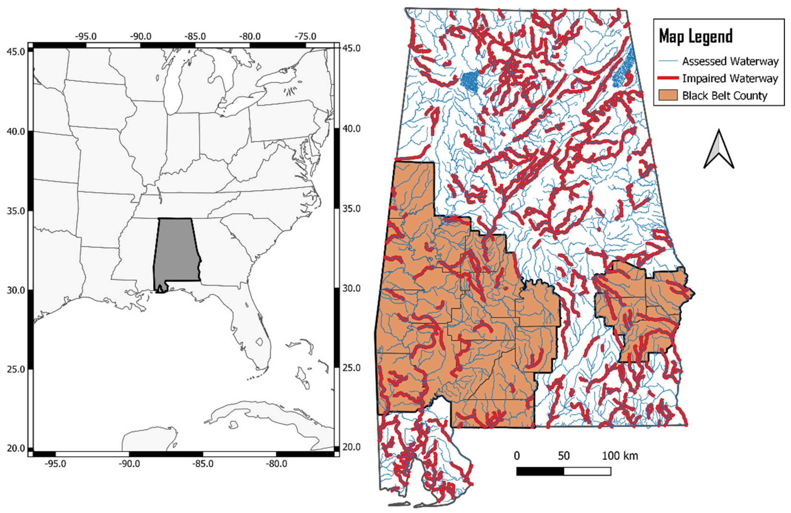
The Alabama Department of Environmental Management monitors water quality and ecosystem health statewide in compliance with the U.S. Clean Water Act. It reports contamination sources and levels to the U.S. Environmental Protection Agency (EPA). The Gulf Intracoastal Waterway system within the Alabama Black Belt includes four major rivers and 22 minor tributaries. It is important to note that because waterways from other areas connect to those in the Black Belt, water quality within the Black Belt may not always be a direct result of commercial, industrial, or agricultural activity within the region. In other words, water pollution and contamination may occur elsewhere upstream and migrate to the Black Belt. Regardless of whether polluting activity occurs within the Black Belt or elsewhere, the most recent data from 2020 shows that of the 20 counties included in our Alabama Black Belt dataset, only one has no impaired waterways [25]. Pathogens and mercury contamination were the most significant contributors to Black Belt waterways impairment at 42% and 34%, respectively.

Determined by elevated counts of E. coli bacteria, pathogen impairment most commonly results from sewage discharges and overflows or failures of septic systems. Septic tank systems are often used in areas where public sewer systems are unavailable. Residents in the Alabama Black Belt are especially vulnerable to their use because of the predominance of clay soils in the region that are not conducive to the filtration necessary for a septic tank system to be effective, often resulting in system overflows and failures.

The EPA reports that more than 40% of Alabama Black Belt households use septic tank systems. Due to poor soil drainage in the region, Black Belt septic system failure rates are among the highest in the country [26]. Such outcomes increase pressure on authorities safeguarding community watersheds and freshwater wells. Nevertheless, septic tank prevalence and the associated problems are not limited to the Alabama Black Belt. It is more widespread and typical in many impoverished areas in the U.S. [27]. Officials in the Black Belt and other areas express similar struggles with septic tank system failures and worry that “compromised septic systems can pollute nearby waterways” [28].

In Alabama, some electrical power is produced by burning coal. Burning coal produces coal ash. Coal ash is dangerous because it contains carcinogenic or hazardous substances, primarily mercury, but also cadmium, lead, chromium, selenium, and arsenic. Coal ash from atmospheric fallout and leaks and overflows from coal ash landfills and ponds contain mercury, a significant source of waterway contamination in the Alabama Black Belt [29].

Power plant operators capture most of the coal ash and place it into landfills or impoundment ponds created by mixing coal ash with water. However, some ash does fall directly into waterways, and some ash makes its way to underground water tables after falling onto land. Further contamination can occur if coal ash leaches from landfills into groundwater or heavy rains cause uncapped coal ash ponds to overflow into nearby rivers and streams.

Environmental and health scientists express concern about storage safety at Alabama’s 15 coal ash disposal sites, asserting that most coal ash has been placed into “unlined, unregulated, and unmonitored ponds and landfills” [30]. Civil rights activists also voice alarm about the placement of Alabama’s coal ash disposal sites in impoverished areas, arguing that outcomes disproportionately affect low-income communities and people of color [31].

Reducing or eliminating mercury contamination is necessary for the Black Belt. Achieving it will be challenging. We argue that in the interest of sustainability of the Black Belt’s water and economies, officials must push forward. The difficulties, of course, are how to balance all concerns. Waterway contamination harms humans and wildlife, yet electricity is the economy’s lifeblood. If it is true that striking a workable balance and trade-offs are necessary, then it must also be true that authentic leadership and impactful action are necessary as well.

2.6. Home Values and Economic Growth in the Alabama Black Belt

Community leaders have long understood the importance of developing and implementing new approaches for reducing poverty, improving quality of life, and stimulating economic growth in the Alabama Black Belt [32]. We argue that one important concept Alabama Black Belt leaders should consider and understand is the long-standing affirmation that home values significantly contribute to economic growth [33,34,35,36,37]. There is substantial empirical evidence highlighting consensus among environmental scientists and real estate economists that water proximity is a positive externality affecting the housing market [8,9,10]. Steinnes [38] even suggests that consumers’ perceptions of degraded water quality could switch their views of waterways as a positive externality to a negative one.

Vital to policymakers and regulators is the essence of it all. Research shows that increased property values associated with high-quality waterways lead to increased local tax revenues and positive economic growth. The opposite is true in areas with impaired waterways.

2.7. Hedonic Pricing Method for Environmental Amenities and the Housing Market

The hedonic pricing method [5,39,40,41,42] is a standard procedure used to assess the value of environmental amenities, or disamenities, based on buyer preferences in property purchase decisions. The purchase outcome reveals choices to buy a bundle of goods that includes housing features, neighborhood attributes, and environmental quality characteristics. Frequently, researchers apply the hedonic pricing method using the housing market as a proxy to measure the marginal value of an area’s environmental quality.

For the 50 years since Rosen [40] first formalized the hedonic pricing method to quantify relationships between the prices of a good and its characteristics, researchers have explored variations of hedonic modeling to examine how property values are affected by proximity to environmental externalities. Some studies focused on positive externalities such as recreational amenity type, surface coverage, and access. Others examined negative environmental externalities such as hazardous waste storage, powerlines, and wastewater treatment facilities. For more in-depth reviews of similar studies, see Boyle and Keil [43], Herath and Maier [44], Owusu-Ansah [45], Palmquist and Smith [46], Sirmans et al. [47], and Xiao [48].

A frequently studied externality impacting the housing market is water quality. However, most hedonic studies examining the relationship between proximity to high-quality waterways and home values use properties located on or near vacation or recreational areas. Research has shown a positive relationship between water quality and prices for Finnish properties on the Baltic Sea and surrounding lakes and rivers [7]. In South Florida, water quality improvements in the Indian River Lagoon, St. Lucie River, and St. Lucie River Estuary are associated with higher property values [9]. In other examples, Maryland consumers are willing to pay more for higher quality water lakefront properties [49]; New Hampshire water clarity positively affects lakefront prices and property tax revenues [50]; water quality is implicitly capitalized in the price of Minnesota lakeshore properties [51]; Chesapeake Bay waterfront buyers pay a premium for higher quality water [52]; water clarity positively affects prices of undeveloped lakefront lots in northern Minnesota [38]; and waterfront property prices increased after the completion of water restoration efforts in Johnson Creek, Oregon, and Burnt Bridge Creek, Washington [53].

2.8. Hypothesis Development

We aim to estimate the impact of proximity to major waterways and minor tributaries of the Gulf Intracoastal Waterway on home values. We do so by casting water quality as a positive amenity. As earlier stated, research shows a positive relationship between water quality and properties on or near the water. We follow similar research paths, as outlined in our literature review, testing the relationship between major waterways and minor tributaries of the Gulf Intracoastal Waterway. We state our hypotheses in the null, as follows:

Hypothesis 1.

Proximity to major waterways of the Gulf Intracoastal Waterway has no impact on the values of homes located in census tracts that cross or are adjacent to major waterways of the Gulf Intracoastal Waterway.

Hypothesis 2.

Proximity to minor tributaries of the Gulf Intracoastal Waterway has no impact on the values of homes located in census tracts that cross or are adjacent to minor tributaries of the Gulf Intracoastal Waterway.

3. Data and Methods

Our study area encompasses 20 Alabama Black Belt counties, including Barbour, Bullock, Butler, Choctaw, Clarke, Conecuh, Dallas, Escambia, Greene, Hale, Lowndes, Macon, Marengo, Monroe, Perry, Pickens, Russel, Sumter, Washington, and Wilcox. We base our econometric analysis on 2016 cross-sectional census tract data derived from consumer surveys of property values and attributes and demographic and socioeconomic characteristics. We merged this dataset with water quality impairment data. All data are publicly available. We express our proxy for water quality as miles of impaired streams (see Figure 1).

Our dependent variable, the median property value of occupied housing units per census tract, estimates home values based on consumers’ preferred prices during a sale. Although such outcomes are unobservable and may suffer from self-reporting bias, our current approach aligns with Arrow et al. [54]. They suggest that “stated preferences” models can assess the impact of environmental externalities. Other researchers also strongly support using the method to assess environmental amenity impacts, and recent evidence shows its use has gained traction within the regulatory framework. Arguing strongly for their use, economist Paul Portney believes contingent valuation methods will be essential to future public policy debate and development [55].

McLean and Mundy [56] argue that real estate appraisers widely accept contingent valuation analysis techniques to assess the value of contaminated properties when historical or recent transactions are unavailable. Contingent valuation models are based on “stated preferences”, the self-reported willingness to pay or receive compensation for damages. Researchers use median property values as a reasonable proxy for an owner’s willingness to sell based on their self-assessment of their property’s value. We argue that our use of a proxy to capture an owner’s willingness to pay for potential externalities is an acceptable approach in the absence of “revealed preferences” transactions.

Econometric Model

The best research methodology to answer our research question is an endogenous, regime-switching hedonic model. The advantage of this model is that it attempts to include a latent process, labeled D*, that reflects the utility a consumer associates with their locational choice of buying a property in a census tract that crosses or is adjacent to either a major waterway or minor tributary. Therefore, if such a process exists, then:

$${\mathit{D}}_{\mathit{i}}^{\mathbf{*}}=\mathit{z}{\mathbf{\prime }}_{\mathit{i}}\mathit{\gamma }+{\mathit{u}}_{\mathit{i}} \mathrm{with} \{\begin{array}{c}{\mathit{D}}_{\mathit{i}}=\mathbf{1} \mathrm{if} {\mathit{D}}_{\mathit{i}}^{\mathbf{*}}>\mathbf{0} \\ {\mathit{D}}_{\mathit{i}}=\mathbf{0} \mathrm{if} {\mathit{D}}_{\mathit{i}}^{\mathbf{*}}<\mathbf{0}\end{array}$$

(1)

where z’_i is a row vector of exogenous variables that could explain a homeowner’s choice to buy property in the census tract that is in proximity to either the Alabama or Tombigbee Rivers “if D_i = 1” or the census tract where only minor tributaries are present “if D_i = 0.” Exogenous factors include population density (POPDENSITY), size of the African American population (POPBLACK), size of the Caucasian population (POPWHITE), median household income (MEDINC), the total number of housing units (HUNITS), number of mobile homes (MOBHUNITS), number of vacant housing units (VACHUNITS), and area covered by water (AWATER).

We use a probit model, simultaneously estimating our discrete choice of Equation (1) with the following endogenous switching equations to model the median property prices that face two regimes. The first, D_i = 1, is the median price of properties located in census tracts that cross or are adjacent to a major waterway. The second, D_i = 0, is the median price of properties in census tracts that do not cross or are not adjacent to a major waterway. Therefore, we express our endogenous regime-switching hedonic model as:

$$ln{\left(\mathit{y}\right)}_{\mathbf{1}\mathit{i}}=ln\left(\mathit{x}\right){\mathbf{\prime }}_{\mathbf{1}\mathit{i}}{\mathit{\beta }}_{\mathbf{1}}+{\mathit{\epsilon }}_{\mathbf{1}\mathit{i}} \mathrm{if} {\mathit{D}}_{\mathit{i}}^{\mathbf{*}}>\mathbf{0} \left({\mathit{D}}_{\mathit{i}}=\mathbf{1}\right)$$

(2)

$$ln{\left(\mathit{y}\right)}_{\mathbf{0}\mathit{i}}=ln\left(\mathit{x}\right){\mathbf{\prime }}_{\mathbf{0}\mathit{i}}{\mathit{\beta }}_{\mathbf{0}}+{\mathit{\epsilon }}_{\mathbf{0}\mathit{i}} \mathrm{if} {\mathit{D}}_{\mathit{i}}^{\mathbf{*}}<\mathbf{0} \left({\mathit{D}}_{\mathit{i}}=\mathbf{0}\right)$$

(3)

where y_i is the median price of the property in logarithmic form in the two regimes; x_1i and x_0i are row vectors of housing attributes and economic, demographic, and environmental characteristics of the census tract i that may have an impact on the median price of the property in the two regimes. These factors, expressed in logarithmic form, include: size of the African American population (POPBLACK); size of the Caucasian population (POPWHITE); median household income (MEDINC); size of the population with a high school diploma (HSDIPLOMA); size of the population with an associate undergraduate degree (ASSOCDEG); size of the population with a bachelor undergraduate degree (BACHDEG); the area covered by water (AWATER); the number of housing units with 1 room (R1); the number of housing units with 2 rooms (R2); the number of housing units with 3 rooms (R3); the number of housing units with 4 rooms (R4); the number of housing units with 5 rooms (R5); the number of housing units with 6 or more rooms (R6PLUS); the number of vacant housing units (VACHUNITS); the number of mobile homes (MOBHUNITS); the number of occupied rented units (HUNITSRENT); the number of properties less than three years old (HAGELT3Y); the number of properties between four and six years old (HAGE4T6Y); the number of properties between 7 and 17 years old (HAGE7T17Y); the number of properties between 18 and 27 years old (HAGE18T27Y); the number of properties between 28 and 37 years old (HAGE28T37Y); the number of properties between 38 and 47 years old (HAGE38T47Y); the number of properties between 48 and 57 years old (HAGE48T57Y); the number of properties between 58 and 67 years old (HAGE58T67Y); the number of properties between 68 and 77 years old (HAGE68T77Y); the number of properties older than 78 years (HAGEGT78Y); and, the miles of impaired waterways (IMPAIREDMILES) (see

Table 1. Descriptive statistics.

Variable	Description	Mean	Std. Dev
D *	1 if the census tract crosses or is adjacent to major Black Belt waterways: Tombigbee or Alabama Rivers; 0 otherwise	66.00	5.81
MEDIANVALUE	Median Property Value (2016 USD)	84,414.07	25,325.93
POPDENSITY	Inhabitants per square mile	257.35	647.44
POPBLACK	Number of African American inhabitants	1592.69	1023.19
POPWHITE	Number of Caucasian inhabitants	1368.81	1134.21
MEDINC	Median Income (2016 USD)	31,619.24	9051.24
HSDIPLOMA	Number of people with high school diplomas	688.58	372.10
ASSOCDEG	Number of people with undergraduate associate degrees	154.29	114.01
BACHDEG	Number of people with undergraduate bachelor’s degree	175.58	152.18
V9	Area covered by water (square miles)	1.33	1.91
R1	Number of housing units with 1 room	19.16	30.13
R2	Number of housing units with 2 rooms	15.18	24.61
R3	Number of housing units with 3 rooms	74.19	75.30
R4	Number of housing units with 4 rooms	242.53	160.68
R5	Number of housing units with 5 rooms	406.98	196.20
R6PLUS	Number of housing units with 6 or more rooms	729.26	382.18
VACHUNITS	Number of vacant housing units	333.22	170.71
MOBHUNITS	Number of mobile homes	369.44	241.37
HUNITSRENT	Number of rented occupied housing units	292.34	273.66
HAGELT3Y	Number of housing units that are less than 3 years old	3.61	9.79
HAGE4T6Y	Number of housing units between 4 and 6 years old	31.86	98.05
HAGE7T17Y	Number of housing units between 7 and 17 years old	165.42	143.98
HAGE18T27Y	Number of housing units between 18 and 27 years old	300.14	165.47
HAGE28T37Y	Number of housing units between 28 and 37 years old	249.44	166.02
HAGE38T47Y	Number of housing units between 38 and 47 years old	267.23	148.97
HAGE48T57Y	Number of housing units between 48 and 57 years old	172.98	115.06
HAGE58T67Y	Number of housing units between 58 and 67 years old	128.19	94.59
HAGE68T77Y	Number of housing units between 68 and 77 years old	68.84	58.77
HAGEGT78Y	Number of housing units older than 78 years	99.59	91.17
IMPAIREDMILES	Impaired river miles within the county superset of census tract	97.75	70.78
Sample Size	Number of census tracts	135

Note: * Binary variable. Mean and standard deviation are computed for the binomial distribution.

for statistical summaries of variables used in our empirical model).

We incorporate a highly efficient estimation by using an algorithm of nonlinear unconstrained optimization (Full Information Maximum Likelihood, or FIML) following Affuso and Lahtinen [57]. Our endogenous regime-switching model enables a counterfactual analysis to estimate the capitalization of the value of waterway proximity into the median property price [58]. This unique empirical design enables us to estimate average median values of properties located in census tracts that cross or are adjacent to a major waterway versus the counterfactual case of properties located in census tracts with no major waterways and vice-versa. A primary advantage of using this approach rather than similar non-parametric methods, such as propensity score matching, for example, is that doing so permits the consideration of other unobservable factors that could also impact property values [59,60]. The present case, for example, could include preferences for waterway type, depth, or width.

4. Results

Because we facilitate numerical optimization of all probit equation variables except for the area covered by water by scaling the variables by 1000, we interpret marginal effects as changes on the order of 1000 units (see

Table 2. Endogenous regime-switching hedonic price model FIML estimates.

	Probit Selection Equation			Regime Di = 1	Regime Di = 0
	Estimates	Marginal Effects		Estimates	Estimates
Constant	0.24 (0.742)	0.082 (1.566)	Constant	12.357 *** (2.314)	5.27 ** (2.239)
POPDENSITY	0.027 (0.464)	0.009 (0.154)	ln(POPBLACK)	−0.013 (0.132)	0.115 (0.09)
POPBLACK	−0.903 *** (0.316)	−0.308 *** (−10.267)	ln(POPWHITE)	0.189 * (0.113)	0.092 * (0.048)
POPWHITE	−0.967 *** (0.357)	−0.330 *** (−9.271)	ln(MEDINC)	−0.152 (0.204)	0.581 ** (0.232)
MEDINC	−0.029 (0.02)	−0.01 (−1.095)	ln(HSDIPLOMA)	0.033 (0.216)	−0.256 * (0.14)
HUNITS	2.268 *** (0.842)	0.773 *** (8.897)	ln(ASSOCDEG)	−0.077 (0.121)	0.111 (0.087)
MOBHUNITS	1.724 * (0.901)	0.587 *** (4.622)	ln(BACHDEG)	0.092 (0.089)	0.029 (0.064)
VACHUNITS	−2.227 (1.511)	−0.759 *** (−12.545)	ln(AWATER)	0.157 ** (0.079)	0.056 (0.07)
AWATER	0.062 (0.125)	0.021 (1.001)	ln(R1)	0.045 (0.026)	0.029 (0.02)
			ln(R2)	0.006 (0.03)	0.008 (0.022)
			ln(R3)	−0.098 ** (0.046)	−0.008 (0.031)
			ln(R4)	−0.28 *** (0.108)	−0.093 (0.101)
			ln(R5)	−0.273 (0.177)	−0.115 (0.137)
			ln(R6PLUS)	−0.113 (0.319)	−0.066 (0.233)
			ln(VACHUNITS)	0.063 (0.152)	0.06 (0.132)
			ln(MOBHUNITS)	0.01 (0.08)	−0.008 (0.054)
			ln(HUNITSRENT)	0.231 ** (0.103)	0.12 (0.079)
			ln(HAGELT3Y)	0.014 (0.05)	−0.017 (0.026)
			ln(HAGE4T6Y)	−0.006 (0.028)	−0.017 (0.025)
			ln(HAGE7T17Y)	0.119 (0.08)	−0.039 (0.065)
			ln(HAGE18T27Y)	−0.036 (0.111)	0.091 (0.105)
			ln(HAGE28T37Y)	−0.006 (0.102)	−0.025 (0.089)
			ln(HAGE38T47Y)	0.001 (0.129)	0.082 (0.103)
			ln(HAGE48T57Y)	0.147 (0.097)	−0.009 (0.078)
			ln(HAGE58T67Y)	0.002 (0.071)	0.028 (0.079)
			ln(HAGE68T77Y)	0.046 (0.05)	0.03 (0.05)
			ln(HAGEGT78Y)	−0.016 (0.053)	−0.069 (0.044)
			ln(IMPAIREDMILES)	−0.008 (0.025)	−0.059 * (0.024)
			σ1	0.21 *** (0.024)
			σ0		0.13 *** (0.02)
			ρ1	0.993 *** (0.001)	NA
			ρ0	NA	0.667 *** (0.001)
Loglikelihood Value	−15.97
AIC	106.1
Degrees of Freedom	66

Notes: *** 99%, ** 95%, and * 90% confidence, respectively. Bootstrapped standard errors in parentheses.

). Statistically significant results suggest that an increase in the number of housing units and mobile homes in census tracts that cross or are adjacent to major waterways increases the likelihood that people will choose to live in these areas by 77% and 59%, respectively. If housing units are vacant, the probability of choosing to live in census tracts that cross or are adjacent to major waterways falls by 76%. We interpret this finding to mean that consumers may perceive such areas as being in economic decline and, if so, look to purchase properties in other areas with more robust economic conditions. Water surface, as measured in square miles, does not seem to be a predictor that drives the choice to live within census tracts that cross or are adjacent to major waterways.

Since our variables are logarithmic, we interpret our reported estimates as elasticities, meaning the percentage change in the average median property value due to one percentage change in the variable (see the last two columns of Table 2). In terms of statistical power, the number of rental units is the main predictor of median property values in census tracts that cross or are adjacent to major waterways. In contrast, median income appears to be a statistically significant predictor for the median property values in census tracts that cross or are adjacent to minor waterways. A 10% increase in median income corresponds to a 5.8% increase in average median property values in those census tracts that are not adjacent to the Black Belt’s major waterways, the Alabama and Tombigbee rivers. Water quality affects only those properties located in areas with minor tributaries connected to the minor waterways (D_i = 0). Our results provide empirical evidence that a 10% increase in pollutants, measured in impaired river miles, corresponds to a 0.6% decline in median property values. Finally, the coefficient of correlation and error terms associated with both regimes are statistically different from zero, providing strong support for our econometric modeling approach.

5. Discussion

Our initial analysis focuses on impaired waterways as environmental disamenity. The estimated econometric model predicts that homeowners living on or near minor tributaries of the Gulf Intracoastal Waterway experience a 0.6% loss in property value per mile of an impaired waterway. This loss corresponds to an approximate per household monetary loss of USD 5065 per mile.

The results of our counterfactual analysis are in stark contrast. By estimating the difference between the predicted average median value of properties located in census tracts that cross or are adjacent to major waterways in the actual case versus the counterfactual case, we can derive a potential measure of the social benefit or cost of living in proximity to a major waterway. The major waterway effect implies that consumers would be willing to sell properties in proximity to a major waterway for USD 22,756 less than if they were not situated on a major waterway, a 22.17% decrease in value (see

Table 3. Counterfactual analysis.

	Actual Case E(Price|Di = 1)	Counterfactual Case E(Price|Di = 0)	Major River Effect
Regime (Di = 1)	79,881 a,*** [73,909; 85,315]	102,636 a,*** [93,757; 110,729]	−22,756 b,*** [−32,791; −12,333]
Regime (Di = 0)	57,327 a,*** [52,686; 61,937]	86,879 a,*** [81,090; 92,239]	−29,552 b,*** [−36,769; −22,183]
Base Heterogeneity	22,554 *** [15,204; 29,629]	15,758 *** [5,455; 25,775]	6,796 c [−5,599; 19,203]

Notes: All values in 2016 USD; *** 99% confidence; bootstrapped 95% confidence intervals in square brackets; ^a H₀: sample mean = 0; ^b H₀: means difference = 0; ^c transitional heterogeneity.

). Our interpretation is that consumers prefer living on minor tributaries rather than major waterways of the Gulf Intracoastal Waterway in the Alabama Black Belt.

As mentioned earlier, this value should be taken as a hypothetical upper bound, given that the median property value is self-reported. In other words, this may likely reflect an upward valuation bias. Even so, the t-test of the difference between the means of the factual and counterfactual scenarios (t-value −4.352) causes us to reject Hypothesis 1, that is, proximity to a major waterway of the Gulf Intracoastal Waterway has no impact on the values of homes located in census tracts that cross or are adjacent to a major waterway of the Gulf Intracoastal Waterway. Hypothetically, proximity to major Black Belt waterways reduces median property values by an average of 34.02%. In contrast, our results suggest that consumers place more value on living near minor tributaries than major waterways.

Of course, other factors could affect home buyers’ locational choices. The available dataset does not have information on other essential factors, such as the quality of school districts, for example, which may affect U.S. consumers’ locational choices. However, base and transitional heterogeneities account for other unobserved factors that may impact property value. For example, homeowners in a census tract near major waterways are willing to sell their property, on average, for USD 22,554 more, regardless of the potential impact of the waterway itself. Similarly, in the counterfactual case in which a property situates in an area with only minor tributaries, on average, the same property owners are willing to sell their property for an additional USD 15,758. These findings then cause us to reject Hypothesis 2, that is, proximity to a minor tributary of the Gulf Intracoastal Waterway has no impact on the values of homes located in census tracts that cross or are adjacent to a minor tributary of the Gulf Intracoastal Waterway. Potentially, these disparities result from systematic variation across the two subsamples not fully captured because of data limitations. Nevertheless, the transitional heterogeneities, which measure whether the effect of the major waterway is more significant for properties in census tracts with major waterways versus only minor tributaries, are statistically equal to zero.

Our analysis suggests that Black Belt property owners prefer homes that cross or are adjacent to minor tributaries over those that cross or are adjacent to major waterways. We compute the aggregate benefit of living in areas with only minor tributaries by summing the home price differential in the factual and counterfactual cases across all the census tracts. In total, the value per census tract is approximately USD 722,512. Our findings confirm earlier discussed prior research that waterfront proximity has a positive impact on home values. However, they also open the possibility that the type of water, particularly the water quality itself, may also play a role in consumers’ locational decisions.

5.1. Data Limitations and Sensitivity Analyses

A significant limitation of the study is the nature of the data. As mentioned in the data section, the dataset consists of aggregate cross-sectional data at the census tract level. The full dataset consists of 135 observations, with a risk of type-2 errors. To test our model’s accuracy, efficiency, and validity, we conducted two experiments: (1) a k-fold cross-validation using machine learning to test model accuracy and efficiency and (2) a non-parametric bootstrap to test whether the asymptotic properties of the estimators hold.

The cross-validation exercise consisted of splitting the entire dataset into a training set (2/3 of the data) of 90 observations and a testing set (1/3 of the data) of 45 observations. These two sets of data were randomly selected k times. In k-fold cross-validation, the training set is used to calibrate the model, and the test set is used for validation. In our k = fold test, we set the number of cross-validations to 10 (k-fold = 10). The coefficient of determination (R²), root mean square error (RMSE), and mean absolute error (MAE) are the statistics commonly used in cross-validation to assess the predictive accuracy of our statistical model (see

Table 4. K-fold cross-validation.

k	R2 Training	R2 Testing	RMSE Training	RMSE Testing	MAE Training	MAE Testing
1	0.994	0.993	0.435	0.449	0.247	0.250
2	0.994	0.993	0.434	0.451	0.246	0.253
3	0.994	0.993	0.429	0.460	0.241	0.263
4	0.993	0.995	0.459	0.398	0.266	0.212
5	0.993	0.994	0.442	0.436	0.252	0.240
6	0.994	0.993	0.427	0.465	0.235	0.275
7	0.994	0.993	0.426	0.467	0.234	0.277
8	0.994	0.992	0.418	0.480	0.225	0.294
9	0.993	0.995	0.455	0.408	0.257	0.231
10	0.993	0.993	0.441	0.437	0.253	0.239
Avg.	0.994	0.993	0.437	0.445	0.245	0.253

). Although the model has more predictive accuracy in the training set, the accuracy in the testing set is not substantially different. The decline in predictive accuracy is 2–3% depending on the statistic that is used for comparison.

We used a non-parametric bootstrap to analyze the efficiency of the endogenous regime-switching model’s parameter estimates and the asymptotic properties of the statistics used for the counterfactual analysis. Following Efron and Tibshirani [61], our bootstrap procedure consisted of 9999 random draws from the empirical data distribution. We used this procedure to estimate the robust standard errors in our endogenous regime-switching hedonic price model FIML estimations (see Table 2) and the 95% bootstrap confidence intervals of the statistics of the counterfactual analysis (see Table 4).

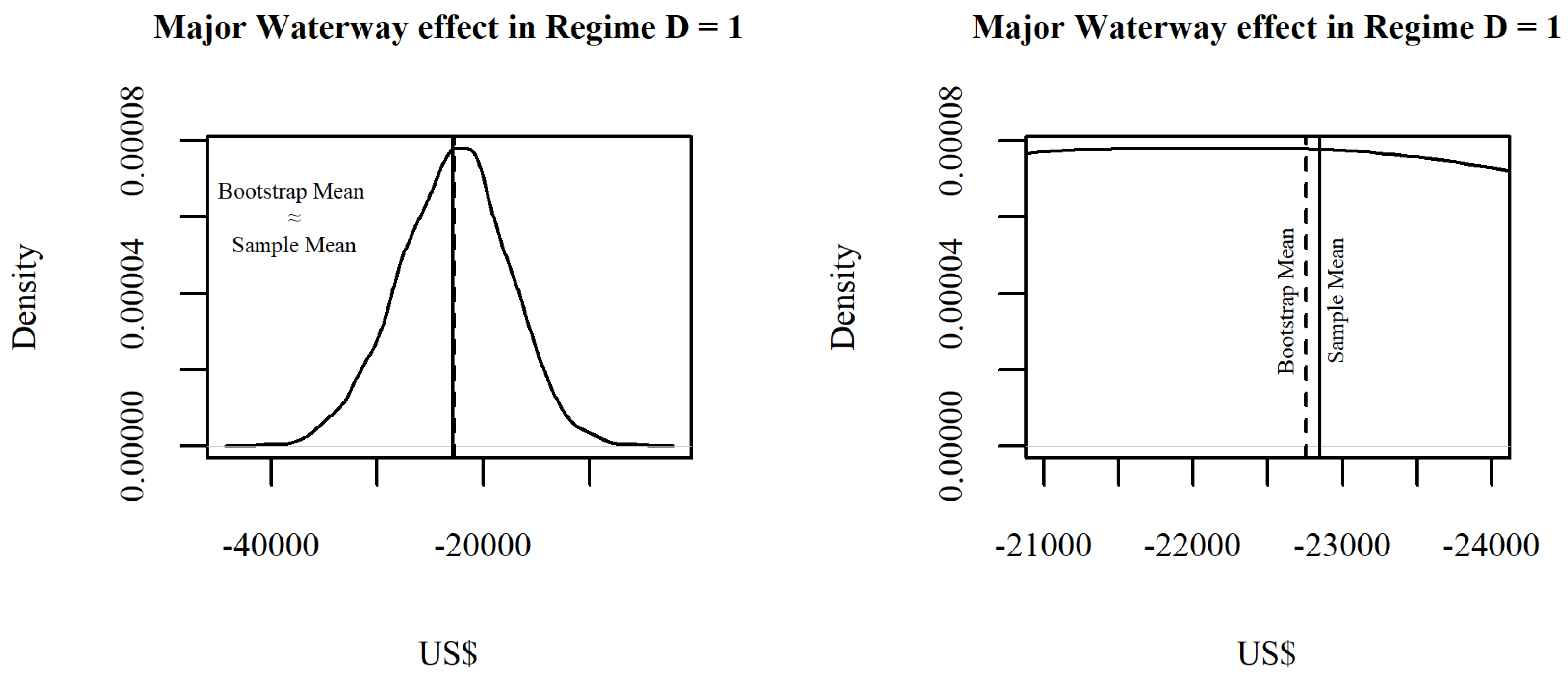
Our asymptotic analysis of the estimators used for the counterfactual analysis clearly shows that, based on a sample of 9999 estimators, the slight sample bias is negligible (see

Table 5. Asymptotic analysis: bias estimation.

	Actual Case E(Price|Di = 1)	Counterfactual Case E(Price|Di = 0)	Major Waterway Effect
Regime (Di = 1)	27.7	−14.93	42.63
Regime (Di = 0)	−21.32	−5.031	−16.29
Base Heterogeneity	49.02	−9.902	58.92

Notes: All values in 2016 USD; bias = bootstrap sample; mean—sample mean.

). For our estimate of interest, the major waterway effect on properties in proximity to major Black Belt waterways, the analysis shows a downward bias (in absolute terms) of only USD 42.63. Hence the biased corrected estimate would be −USD 22,798 ≈ −USD 22,756. The empirical distribution of this statistic is approximately normal with the bootstrap, and the sample means are also quite close (see Figure 2). Hence, we feel confident that the estimated parameters and statistics are still efficient and accurate even in a limited dataset.

5.2. Implications and Generalization

Our study’s contributions to the literature are significant because they call attention to reasons to foresee, identify, and safeguard against any waterway-impairment-related property value declines that may harm area economies [62]. Our goal is to expand clarity about commercial marine waterways’ impacts on housing markets and economic growth in the Alabama Black Belt. We argue that our efforts can serve as a framework for analysis in other areas beyond the Black Belt and yield valuable analytical insights for policymakers and regulators in their work toward sustainable development solutions that balance the interests of commerce, communities, and private property owners.

5.2.1. Implications and Generalizability: Sustainable Development and Water

Just as the United Nations does at an international level, leaders in other areas, at all levels, must continue to persuade and convince their constituents to gain greater awareness and education about sustainable development and the role it plays in the well-being of the planet and humankind. All the United Nations’ 17 sustainable development goals are essential, but water is critical to physical survival.

Discovering new freshwater sources, reusing greywater where possible, and expanding desalination processes should be important priorities. However, at the top of the list is reducing and eliminating water contamination wherever possible. Without question, the world population is increasing. More people will buy more things. Supply chains and global trade will grow more complex. Aggregate effects will increase demands and pressures on global water resources. Taking better care of what we have makes perfect sense. It truly is a matter of survival.

5.2.2. Implications and Generalizability: U.S. Inland Waterway System

The U.S. inland waterway system is a vital infrastructure resource. Its capacity for transporting cargo is unmatched and, in some way, touches the lives of millions of people each day. It may be easy to take for granted that freight and cargo just ‘get delivered.’ Well, perhaps before COVID, it might have been easy. If nothing else, the pandemic has taught people across the globe everything they might ever want to know about the vast complexities of global supply chains.

While beyond the scope of this paper, we were interested to learn in our research that the waterway system’s 237 lock and dam systems are old; many require long-delayed maintenance overhauls, a few are even nearing the point of failure, and, of course, repair and replacement costs are enormous and increasing. If lock and dam systems do not function correctly, barges can run aground and possibly increase the risks of waterway contamination. Malfunctioning locks produce transit delays, driving up supply chain costs. Again, a much broader subject than space permits, but on so many levels, the sustainability of both water quality and the related economies associated with the U.S. inland waterway system is crucially important.

5.2.3. Implications and Generalizability: Gulf Intracoastal Waterway in the Alabama Black Belt

Likewise, as a vital part of the U.S. inland waterway system, maintaining the Gulf Intracoastal Waterway must not be ignored, and ensuring sufficient depths is most important. Even though the Black Belt region does not receive any direct economic benefits from the cargo that is transported on the waterway, there are economic benefits for the residents and community businesses from the related jobs and spending associated with the waterway. Our results show that people value the properties in proximity to minor tributaries of the waterway, so continued waterway access to these properties will be necessary. As any reduced or restricted access could potentially harm property values and the area economy, policymakers must ensure that waterway depths are good; at the same time, from start to finish, all work should conform to best practices for ecological disposal of dredge spoils.

5.2.4. Implications and Generalizability: Impaired Waters in the Alabama Black Belt

In some ways, containing contamination and reversing waterway impairment seem insurmountable challenges. The most significant threat to high water quality in the Alabama Black Belt is contamination from pathogens. It is one thing for officials to instruct residents to fix their failing or failed septic tank systems or risk civil penalties. It is another to make it happen. Given Black Belt soil conditions, the systems with the best chance of working would be those engineered for above-ground installation. Costs would be as much as some people in the Black Belt make in a year. Sadly, many in the region are extremely poor and cannot afford to buy new or upgraded systems. Without large-scale efforts to secure the considerable funding needed to correct deficiencies and change peoples’ lives, things are unlikely to improve soon.

Reducing or eliminating mercury contamination is necessary for the Black Belt. Achieving it will be challenging. We strongly argue in the interest of the sustainability of the Black Belt’s water and its many community economies and urge officials to push forward together, even amidst the challenges of balancing all concerns. We acknowledge how difficult progress will be. Waterway contamination harms humans and wildlife; yet, electricity is the economy’s lifeblood; neither is mutually exclusive. If it is true that trade-offs are necessary to strike a workable balance, then it must also be true that authentic leadership and impactful action are necessary as well. We call for both now.

5.2.5. Implications and Generalizability: Waterfront Home Values in the Alabama Black Belt

Our results reveal that people place great value on owning properties in proximity to the minor tributaries of the Gulf Intracoastal Waterway. Higher Black Belt property values are the result. A possible implication might be that homeowners prefer properties on or near minor tributaries because of perceptions that the water quality is better than on major Black Belt commercial waterways. If so, this would be consistent with the earlier reviewed extensive literature that shows a positive correlation between water quality and property prices. Policymakers and local officials should appeal to water management agencies to enforce the highest water quality standards. Doing so will help maintain and preserve the marine environment and support property values. This is important because of the more significant connection, as noted in the earlier discussion, that strong property values are critical to a community’s economic well-being.

5.3. Opportunities for Future Research

Our study only examined one area of the Gulf Intracoastal Waterway, the Alabama Black Belt. The waterway is over 1100 miles long and is part of the more extensive 12,000-mile U.S. waterway system. Hundreds of communities are spread over these many miles, and while many may be poor areas such as the Black Belt, others may be better positioned. Several ideas come to mind for further research. For example, research on the impacts of water quality, economic strength, racial and ethnic influences, and varying city sizes on housing might be of interest. Perhaps impacts on commercial properties or significant ports might also be of interest. Other studies that incorporate sustainability issues should also be pursued.

As the world struggles through the highest inflationary period in 50 years, an overarching concern is the cost and availability of energy. High energy prices and threats to future energy supplies are forcing leaders worldwide to rethink their climate change strategies and adjust to the real needs of their citizenry. Shippers use the Gulf Intracoastal Waterway to move large cargoes of coal for energy, petrochemicals for plastics, and grain for food products. As populations increase and general economic demand for goods and services rises to keep pace, more shipping will occur on the Gulf Intracoastal Waterway and beyond. Perhaps studying the economic impacts of other waterways in other towns would be interesting. The environmental connection should be clear and viewed as an amenity choice.

Shipping is outsized in marine commerce, interacting with the marine environment like no other industry. Marine safety and marine contamination were not a direct part of this article, but both areas might be exciting research possibilities. For example, how does shipping work economically, and how does it take steps to comply with environmental regulations? What does the supply chain look like at a granular level? What effects do different multipliers have on the different economic scenarios? What about the economic impacts of specific industries’ effects on economic events, such as shipbuilding or repairing? Ship repair companies must use caution when removing marine paints so that the threat of contamination can be examined or evaluated using the same type of counterfactual analysis as we used in this study.

Finally, although this manuscript is not about econometrics, our econometric method choice was integral. We encourage the consideration of endogenous, regime-switching hedonic price modeling. The design is instrumental when research questions dictate gauging the value of relationships dependent on variations within distinct event possibilities, “two regimes”.

6. Conclusions

Earlier, we offered strong support for the positive links between water quality and the housing market. We also pointed out that the large body of research to date has focused primarily on vacation or recreational types of properties. We address this omission by examining how water quality in a commercial marine environment, namely, the Gulf Intracoastal Waterway, impacts the housing market. We use a unique, endogenous regime-switching hedonic pricing method that allows consumer location selection analysis and permits a counterfactual analysis to measure price differentials between properties on impaired major waterways versus those on marginally impaired minor waterways. The goal is to assess how proximity to impaired waterways impacts home values. In doing so, we hope to emphasize the importance of sustaining and preserving the highest water quality possible in the Black Belt’s many waterways.

Although our analysis may be affected by some degree of self-reporting bias, our results suggest an undeniable perception that Black Belt property owners view proximity to minor water tributaries as an environmental amenity. Our counterfactual analysis shows that properties in census tracts that cross or are adjacent to Black Belt major waterways could depreciate by approximately 22% compared to the counterfactual case in which the same properties are in areas with only minor tributaries. Crucially, properties in areas with only minor tributaries could experience value depreciation of as much as 34% if they were counterfactually situated in the proximity of major waterways. We provide empirical evidence that Black Belt homeowners view proximity to minor tributaries as a social welfare benefit equivalent to approximately USD 29,000 per household, totaling an average of USD 722,512 per census tract. Black Belt homeowners also view water quality degradation as an environmental disamenity in areas close to minor tributaries. The social welfare cost associated with waterway impairment amounts to USD 5065 per mile per household.

As future economic prosperity and quality of life for all Black Belt residents depend in many ways on the sustainability of its waterways, policymakers and environmentalists must work together to safeguard these precious, vital environmental resources. In their push for strategies that promote economic growth and create new jobs, policymakers must not overlook the need to strike the right balance between economic and environmental sustainability.