Experimental and Numerical Prediction of Wetting Fronts Size Created by Sub-Surface Bubble Irrigation System

Abstract

A bubble irrigation system (BIS) is a subsurface irrigation method recently introduced that may provide a better mechanism in terms of flow regulation, as it involves mainly the exchange of water and air bubbles under slight negative pressure. The negative pressure flow was created using inverted closed plastic bottles (ICPB) that connected to an elevated closed tank. Understanding the characteristics of wetting fronts is key in designing this irrigation system. This paper mainly presents the principles of BIS, the experimental measurements and software simulation of BIS wetting patterns, and the development of statistical models for BIS wetting patterns dimensions estimation. Laboratory experiments were accomplished to measure the BIS’s sharp-wetting fronts variation with four diameters of contact areas of ICPB and two different soil types, namely SS1 and SS2. In addition, numerical simulations using a 2D HYDRUS were performed to explore the possibility of using the simulated non-sharp wetting fronts in predicting BIS wetting fronts. The experimental results and numerical simulations show that the soil properties and the area of contact have a significant impact on the bubble flow rate and the shape and size of the wetting patterns. The hydraulic conductivity and the density of soil SS2, which were 62 and 22 percent, respectively, higher than soil SS1, have resulted in average incremental ratios of wetted depth and width by 94 and 178 percent, respectively. Results also show that more than 50 percent of the growth of wetting fronts’ width and depth occurred rapidly at the early portion of irrigation time before flattening at the latter time, indicating the effectiveness of the air–water exchange in regulating the amount of water supplied and in controlling wetting fronts propagation. Furthermore, based on experimental and simulation results, regression models have been developed for estimation of bubble flow rates and the size of wetting fronts. The developed models can be reliably used to predict the bubble flow rate and size of wetting patterns with high accuracy.

1. Introduction

Subsurface irrigation systems deliver water directly into the root zone either by free-flow or pressurized flow to reduce losses [1,2,3]. The movement of water in this irrigation system usually starts from the source to the emitters and then moves to the root zone. Researchers have classified the source as a point source [4], line source [5], or area source [6].

Free flow occurs when the intensity of application is equal to or less than the infiltration capacity of the soil [7,8] while pressurized flow is when the application intensity is larger than the infiltration capacity of the soil [9]. The performance of these techniques was widely discussed, analyzed, and modified by many researchers [10].

Recently, a new subsurface flow technique, named the bubbles irrigation system (BIS) was suggested by Alrubaye, et al. [11]. The main principle of BIS is using an air–water exchange mechanism between the voids in the root zone and the ICPB. This mechanism provides the control condition to BIS, which prevents the excessive supply of water into the root zone. In contrast to existing subsurface irrigation techniques, BIS flows under negative pressure, which will not allow the water flow to occur unless bubbles from soil voids come out. The behavior of wetting fronts propagation by this air–water exchange mechanism of BIS has been confirmed to be different from the conventional subsurface irrigation techniques [11].

The wetting front shows the region in which the irrigation water is distributed in the root zone of the soil. In the irrigated zone, the soil is saturated, and the wet region is enclosed by a sharp boundary [12] which is termed a sharp wetting front. According to Lu and Likos [13], the sharp wetting front spreads rapidly at first across the soil and gradually decelerates over time. Conversely, a non-sharp wetting front has a variable moisture content profile during water application [13,14].

Prediction of the size of the wetting patterns is essential for the efficient design, operation, and management of irrigation systems [15]. Moreover, application time, emission rate, and irrigation interval can be determined based on the size of wetting patterns [16].

Among popular models to estimate the size of wetting fronts produced by conventional subsurface irrigation systems are the Green and Ampt [17] and the Richards [18]. Ben-Asher and Charach [19] also introduced the equivalent radius of hemispherical shape that represents the shape of sharp wetting fronts, as in Equation (1):

$$r_{eq}={\left[\frac{1.5*q*t}{\mathsf{\pi }\left(\theta s-\theta i\right)}\right]}^{\frac{1}{3}}$$

(1)

where: r_eq is the equivalent radius of the wetting front, cm; q is the application flow rate, cm³/min; t is the time of application, min; θ_s is the saturated moisture content of the soil, cm³/ cm³; and θ_i is the initial moisture content, cm³/cm³.

Until now, research has revolved around the development of statistical, mathematical, or empirical models for wetting pattern prediction resulting from the emitters of drip irrigation systems [20,21,22,23,24]. Furthermore, laboratory measurements and simulations of wetting patterns have been conducted to design and evaluate the performance of the new improved techniques, such as line source irrigation [25], a vertical moistube-irrigation [26], ceramic emitters [27,28,29,30], subsurface membrane irrigation [31], and ring-shaped emitter for subsurface irrigation [32].

In summary, the wetting front’s prediction for the free and pressurized flow of subsurface irrigation has been explored substantially. Since the BIS is still new and working with a different water application concept, the characteristics of the wetting front patterns created by this system need further investigation.

This paper presents the concept governing the BIS, laboratory measurements of wetting front patterns created by specially designed water–air bubble emitters, numerical simulations of BIS with non-sharp wetting fronts, and a statistical model to predict the size of the wetting patterns for the bubble irrigation system.

2. Materials and Methods

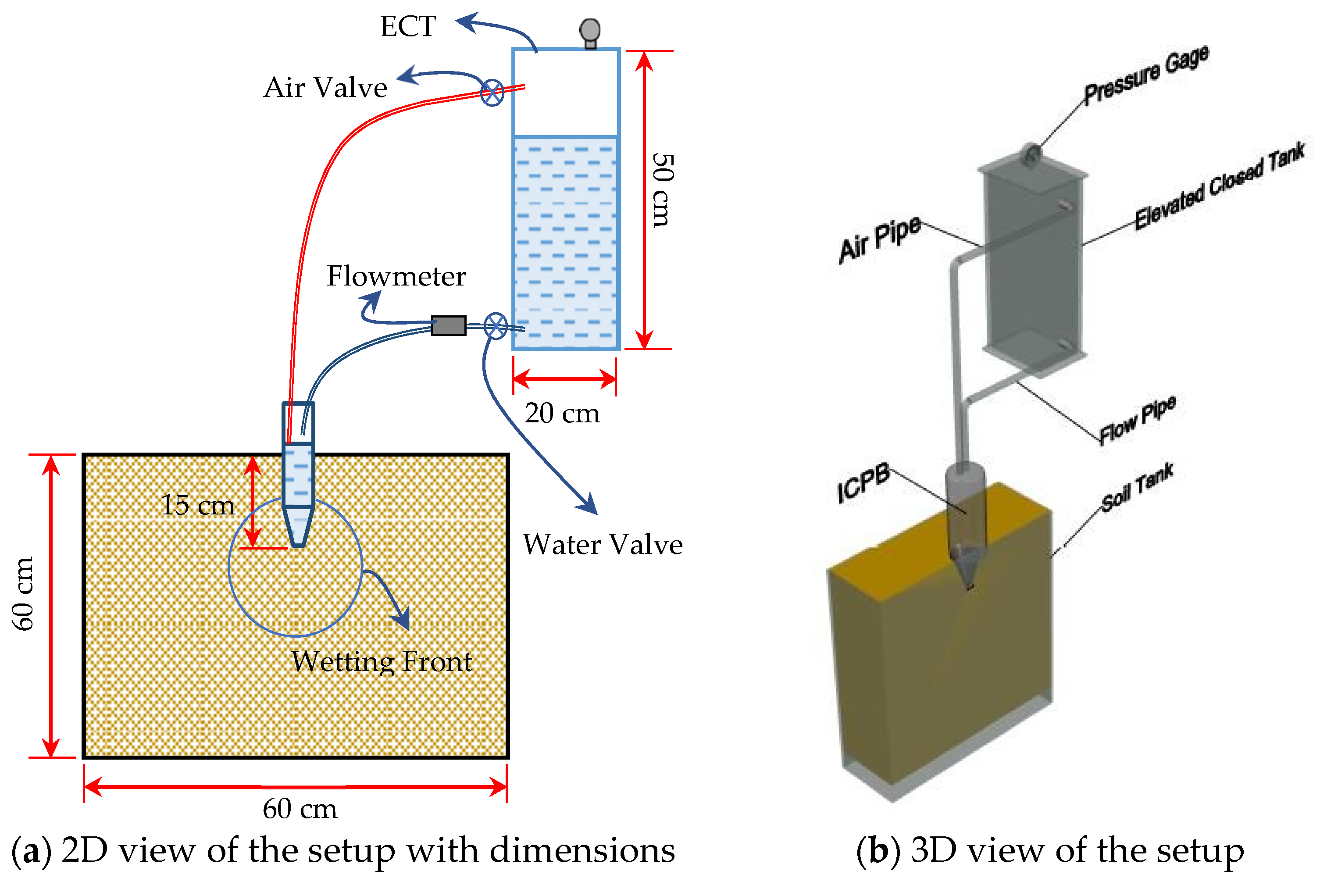
2.1. Experiments

Laboratory experiments were performed to measure the size and shape of wetting fronts created by BIS. The experiments present a 2D unsaturated flow profile in soil. The experimental setup comprised an elevated closed tank (ECT), soil container, and ICPB, as shown in Figure 1. Two soil types and four different diameters of contact area, D_i, were evaluated to present the impact of soil properties with different infiltration areas on the shape and size of wetting fronts in the soil.

Main tools and equipment used in the experiments were: 20 liters ECT, mechanical flowmeter, vacuum pressure gauge, inlet and outlet valves, air valve, 4 sizes of ICPBs, and a glass soil container (60 cm long, 30 cm wide, 60 cm deep, and 5 mm thick).

The ECT and ICPB were connected via two tubes with check valves. One tube was for the air flow and the other for the water flow. To create a closed system, both ECT and ICPB were fully sealed by silicon and Teflon tape. The closed system allowed the air–water exchange and the control of the water supply into the ICPB. A slight vacuum was produced in the ECT during the air–water exchange process. The condition inside the ICPB is fully controlled by the condition in the closed tank. When water levels in the ICPB reach the air tube and block the air flow to the ECT, the ECT automatically stops providing water into the ICPB.

Experiments were performed in the Hydraulic Laboratory of the Department of Civil Engineering, UPM. The soil tank was first filled with soil, layer by layer, to ensure uniformity in compactness and density of the soil. Then, the ICPB was inserted 15 cm into the soil. Water was allowed to fill the ICPB by opening the water valve, generating vacuum pressure in the ECT equivalent to the head between the water table in ECT and ICPB. The discharge and wetting fronts propagations were recorded for every 10 minutes for the first hour and every 30 minutes for the rest of the test duration. During each test, the discharge was measured volumetrically and the wetting front dimensions with time were traced on a transparent sheet. The wetting front propagations were observed in two types of sandy soils, namely as SS1 and SS2. Details of experimental cases are summarized in

Table 1. Experimental Details.

Cases	Diameters of Contact Area, Di. cm	Soils
1	2	SS1 and SS2
2	2.5
3	3
4	4

.

Basic soil tests have been accomplished to measure hydraulic conductivity, k_s, initial moisture content, θ_i, moisture content at field capacity, ${\theta }_{fc}$, and the texture of the soils. The basic soil tests include the constant head test to measure the hydraulic conductivity, the digital moisture meter to measure the initial moisture content, the volumetric method to measure the moisture content at field capacity, and the sieve analysis to define the texture of the soil. The properties of the soils determined from the soil tests are presented in

Table 2. Results of basic experiments of soil properties.

Soil Type	Texture			ks, cm/h	Bulk Density, gm/cm3	θi	θ fc
	Sand	Silt	Clay
SS1	92%	8%	0%	1.19	1.19	5%	58%
SS2	97%	3%	0%	1.85	1.45	5%	33%

.

2.2. Description of Bubbles Flow from ICPB

In BIS, the irrigation application rate and the wetting front propagations are controlled by the air–water exchange in the ICPB. Water flows from ICPB and infiltrates into the soil through the ICPB opening which represents the source contact area with the soil. This process happens only when air bubbles are flowing out from the soil voids to ICPB. This mechanism produces slight vacuum pressure in the ICPB which controls the head of water in the ICPB. The irrigation application rate is highly dependent on the hydraulic properties of soil and the contact area of ICPB, which are the hydraulic conductivity of the soil and the source contact area at the opening of ICPB. Because the infiltration capacity of soil and the size of the wetting patterns varied with time, the water application rate also varied with time. Therefore, the variables that impacted the average flow rate of the bubble source for one hour of application time can be represented by the hydraulic conductivity of the soil, $k_s$, and the diameter of the contact area, D_i.

A model representing the size of BIS’s wetting fronts was developed by adding modification factors to Equation (1), which are based on the following assumptions: (i) the flow from the source area is radial flow; (ii) soil–water movement follows the strong wetting fronts that distinguish the saturated and unsaturated regions; (iii) soil is homogeneous and uniform; and (iv) soil is at its initial moisture content at the beginning of irrigation. Figure 2 shows the schematic of wetting fronts created by ICPB.

The depth and width of the wetting front give major indications of its dimensions and they are the most relevant parameters to be included in the design and management of irrigation systems [33]. In addition, because water movement in the soil is non-isotropic, a change in the shape of the wetting front was produced to precisely anticipate the dimensions of the wetting front over time. The modification considers a non-isotropic soil in the estimation of depth, z, and the width, w, of the wetting front using linear regression analysis. The suggested models for depth and width of the wetting front are shown in Equations (2) and (3), respectively:

z = A + r_eq. B

(2)

w = C + r_eq. D

(3)

where: A, B, C, and D are the model shape modification factors (cm).

Shape modification factors are used to adjust and convert the equivalent wetting front radius to the BIS wetting front shape dimensions in terms of width and depth. The shape modification factors also take into consideration the hydraulic properties of the soil that affect the water and airflow in the soil voids [34] and hence the shape of water distribution from BIS and the variation of the contact area of ICPB that provides the variation of air–water exchange mechanism and different shapes of wetting fronts. The shape modification factors, A and B, were determined using the linear regression analysis method.

In order to use the equivalent radius of the BIS to find the w and z of wetting fronts, it is required to predict the bubble flow rate. In this paper, the diameter of the contact area and hydraulic conductivity of the soil were used as independent variables to predict the bubble flow rate. Linear relation form is proposed between the predicted bubble flow rate and these two independent variables. The statistical model of the predicted flow rate can be written as in Equation (4). The function of this equation is to estimate an average value of bubble flow rate to use it for finding the equivalent radius of wetting fronts:

$$Q={\beta }_o+{\beta }_1. D_i+{\beta }_2.k_s$$

(4)

where: Q is the average predicted flow rate of ICPB, Lph; $D_i$ is the diameter of contact area, cm; $k_s$ is the hydraulic conductivity of the soil, cm/hr; ${\beta }_o$, ${\beta }_1$, and ${\beta }_2$ are the statistical parameters. Linearized multi-regression analysis method has been used to find the parameters of the suggested statistical model for the bubble flow rate.

2.3. Statistical Evaluation of the Linear Regression Modelss

The accuracy of the linear regression models and modification factors established for Equations (2)–(4) has been assessed using a t-test with a 95 percent confidence coefficient. For instance, the null hypothesis assumed that the mean value of the predicted dependent variable is not equal to the mean value of the actual dependent variable. Moreover, other statistical evaluations using root mean square error (RMSE) and multicollinearity test using variance inflation factor, VIF, were performed using R-studio software. RMSE and VIF are presented in Equations (5) and (6):

$$\mathrm{RMSE}=\sqrt{\frac{\mathrm{SSE}}{n}}$$

(5)

$$\mathrm{VIF}={\left(1-R_k^2\right)}^{-1}$$

(6)

where: SSE is the sum square of error, n is observations, and $R_k^2$ is the coefficient of multiple determination when the diameter of the contact area, D, is regressed on the hydraulic conductivity.

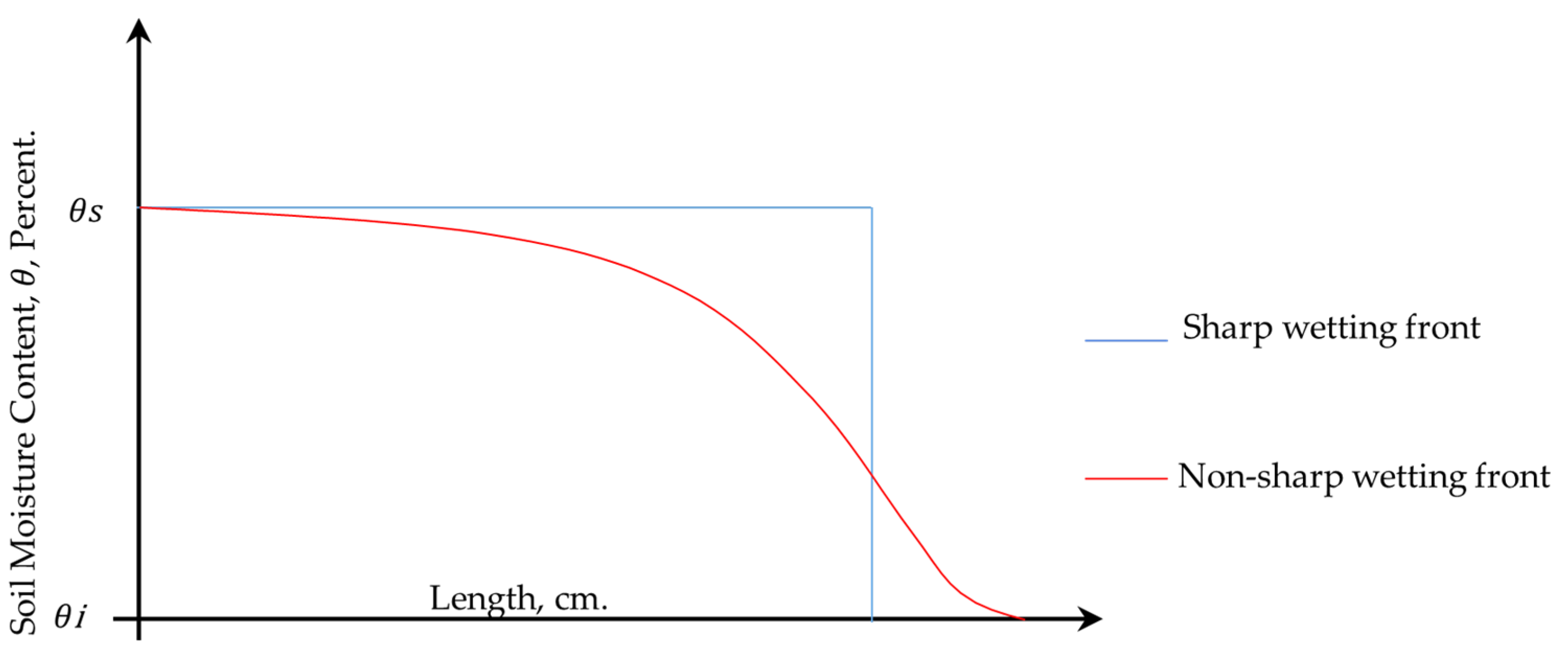
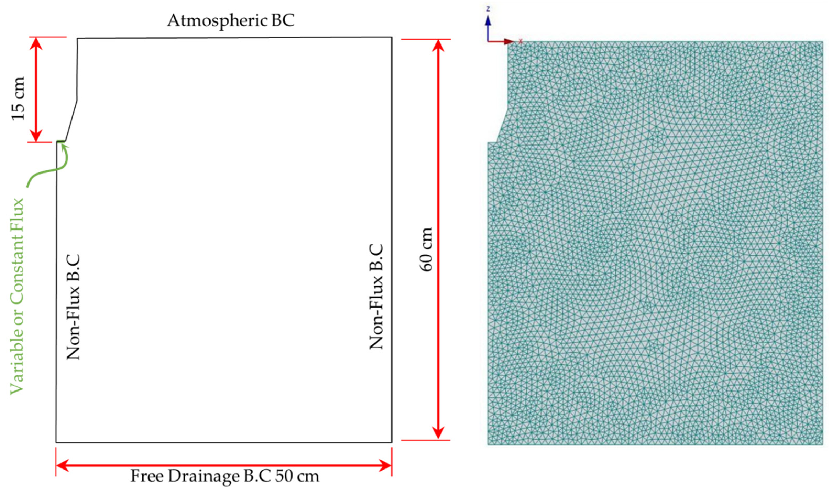
2.4. Estimation of Non-Sharp Wetting Fronts Resulting from ICPB by 2D HYDRUS

This study also explores the possibility of using 2D HYDRUS in predicting the BIS wetting pattern by introducing modification factors to the simulated results. The use of software enables tests in a wide range of conditions to be carried out in more detail and faster than is possible with experiments. HYDRUS is a software that provides a fast and accurate way for investigating soil water dynamics simulations. It has been widely applied in simulating various subsurface irrigation techniques, but its application in simulating BIS is yet to be tested. The soil–water distribution in 2D HYDRUS numerically solves the equation of Richards [18] for two-dimensional flow in soil by finite element method and used the model of Van Genuchten [35] for soil hydraulic properties. The unsaturated flow in soil from ICPB was simulated by the 2D HYDRUS utilizing the variable and constant bubble flow rate boundary conditions.

Wetting fronts behave as a sharp front when the infiltration flux is less than the transition flux, and as a diffused or non-sharp front when the infiltration flux is more than the transition flux, according to DiCarlo [36]. A sharp wetting front created by emission products is usually used for designing proposes [37].

Simulation of the flow of ICPB in 2D HYDRUS produced non-sharp wetting patterns. To relate sharp wetting fronts obtained from the experiment to the simulation results, it is vital to show the interception between sharp and non-sharp wetting patterns. The length of sharp wetting fronts measured from the experiments can be used to find the interception of moisture content of non-sharp wetting fronts that have been simulated by 2D HYDRUS. Figure 3 shows the schematic of interception between sharp and non-sharp wetting fronts.

The unsaturated BIS flow was simulated using 2D HYDRUS software using varied and average constant flow rates as input data to observe the best way of predicting the moisture distribution. The moisture distribution in depth and in width have been produced using vertical and horizontal sections to the infiltration area. The four contact areas with the two types of soils, SS1 and SS2, that were used in the experiments have been used as a basis for the numerical simulations. The boundary conditions used for the simulation were variable or constant flux, atmospheric, non-flux, and free drainage boundary conditions. Figure 4 shows the boundary conditions of the flow region and the finite element meshes.

To simulate the experimental cases in 2D HYDRUS, initial moisture content, ${\theta }_i$, has been used as equal to the residual moisture content. Soil hydraulic parameters of Van Genuchten [35], such as residual moisture content, θ_r, and saturated moisture content, θ_s, empirical coefficients affecting the shape of hydraulic function, α and n, and pore connectivity parameter, l, were predicted using the neural network prediction option in 2D HYDRUS. Rosetta Lite v. 1.1 in 2D HYDRUS has been used to predict the soil hydraulic parameters of the soils according to the soil texture, bulk density, and moisture content at field capacity. The soil hydraulic parameters used in this simulation are shown in

Table 3. Soil hydraulic parameters used for 2D HYDRUS simulations.

Cases	Soil Type	Di, cm.	θr, cm3/cm3	θs, cm3/cm3	α	n	ks, cm/min	l
1	SS1	2	0.1053	0.5071	0.05	2	0.01979	0.5
2	SS1	2.5	0.1053	0.5071	0.05	2	0.01979	0.5
3	SS1	3	0.1053	0.5071	0.05	2	0.01979	0.5
4	SS1	4	0.1053	0.5071	0.05	2	0.01979	0.5
5	SS2	2	0.0473	0.415	0.0032	2.7	0.03087	0.5
6	SS2	2.5	0.0473	0.415	0.0032	2.7	0.03087	0.5
7	SS2	3	0.0473	0.415	0.0032	2.7	0.03087	0.5
8	SS2	4	0.0473	0.415	0.0032	2.7	0.03087	0.5

.

3. Results and Discussion

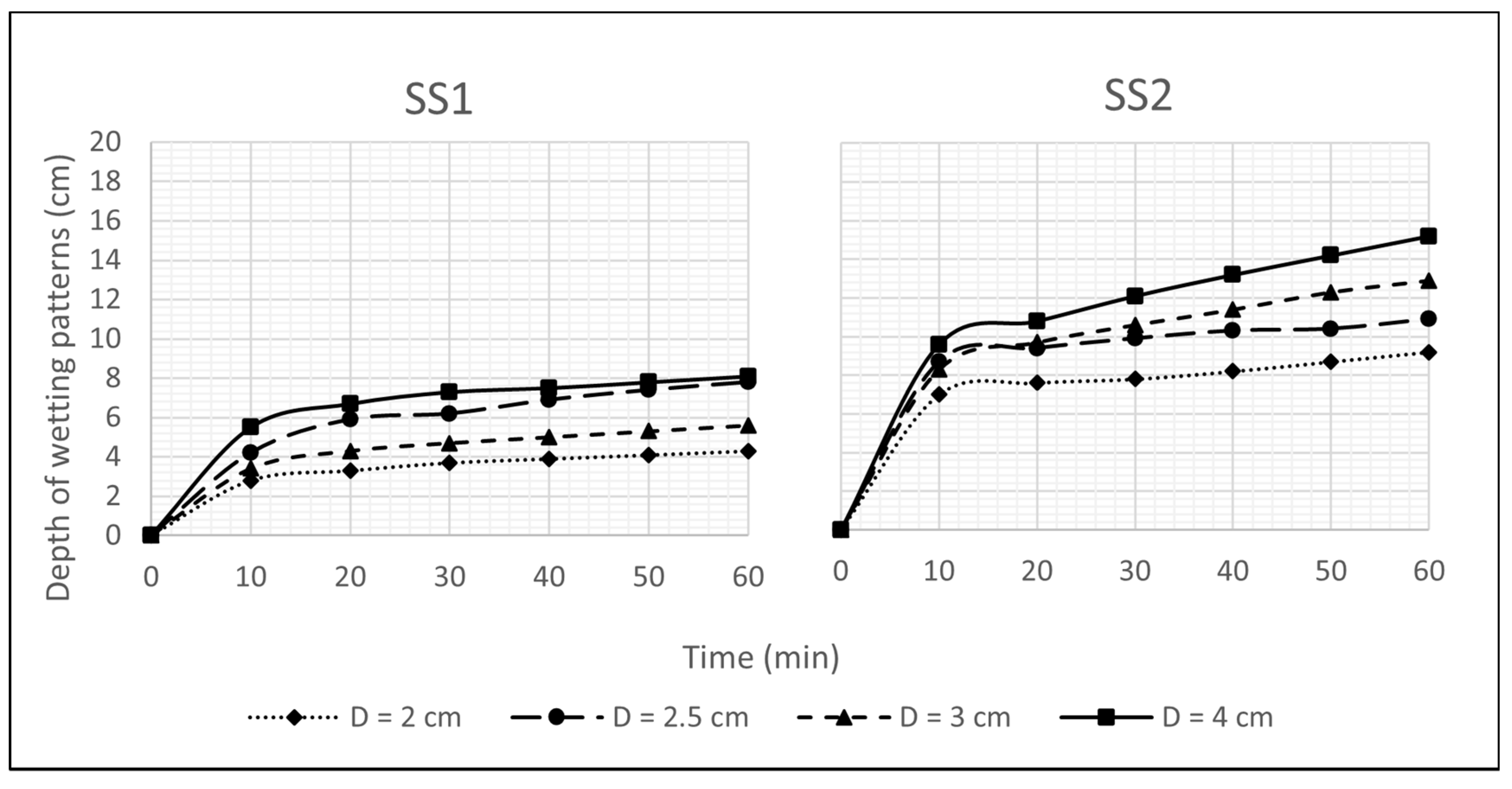
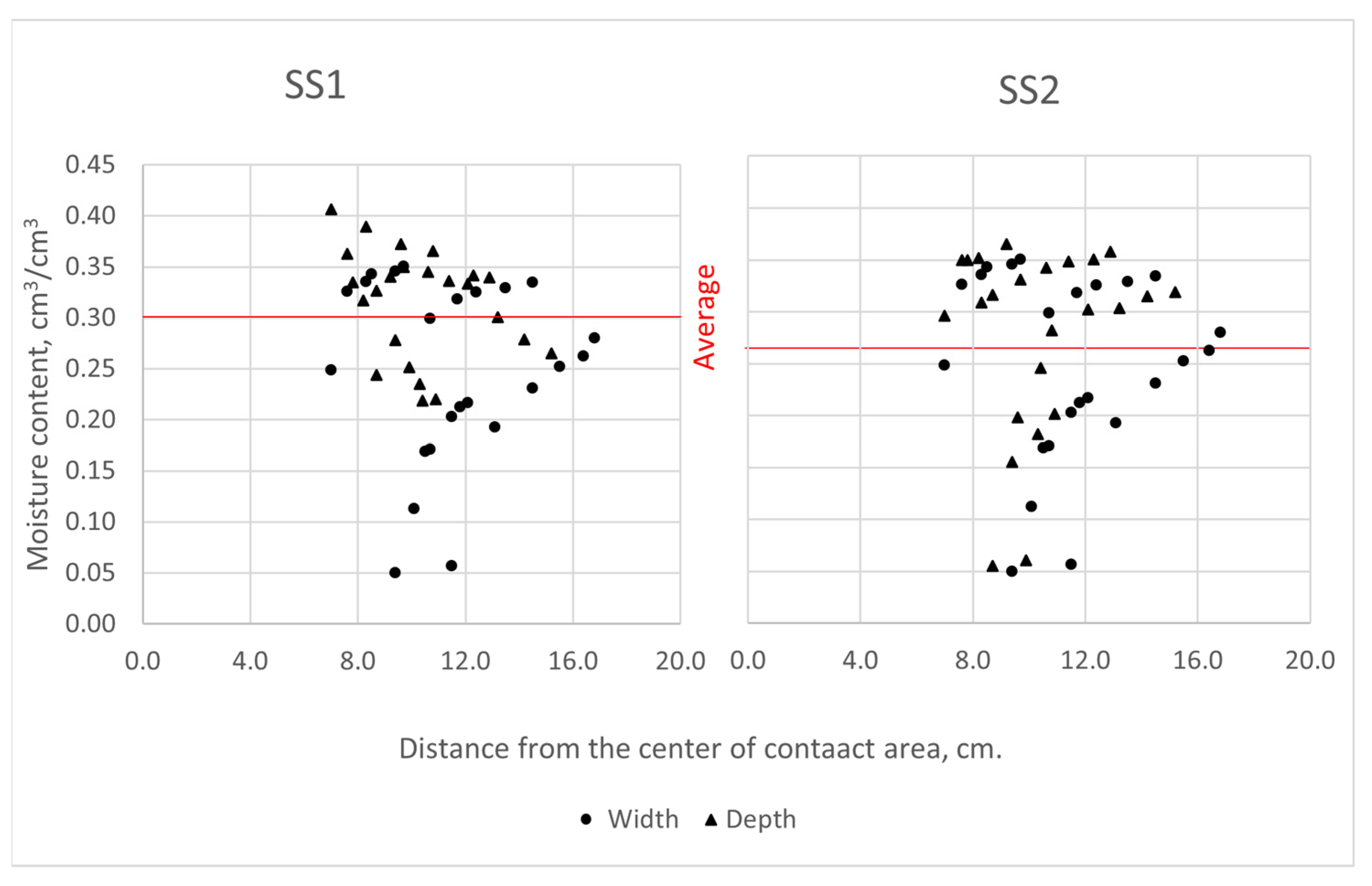
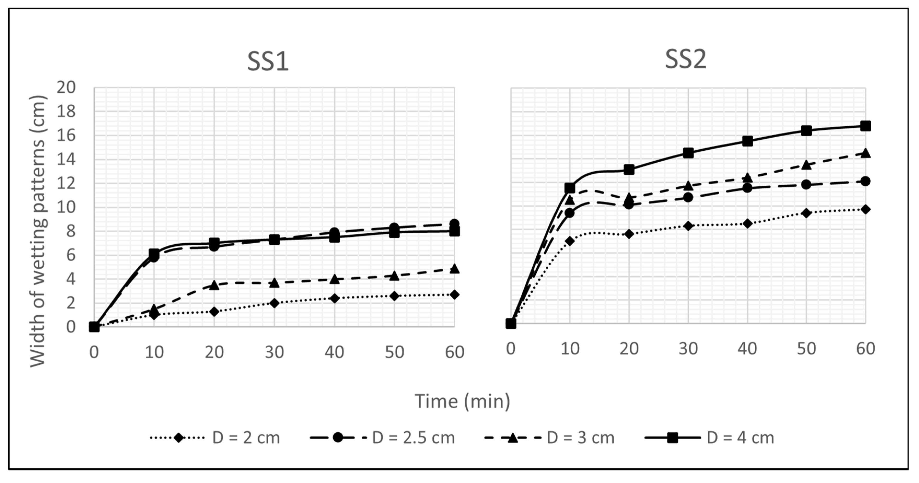
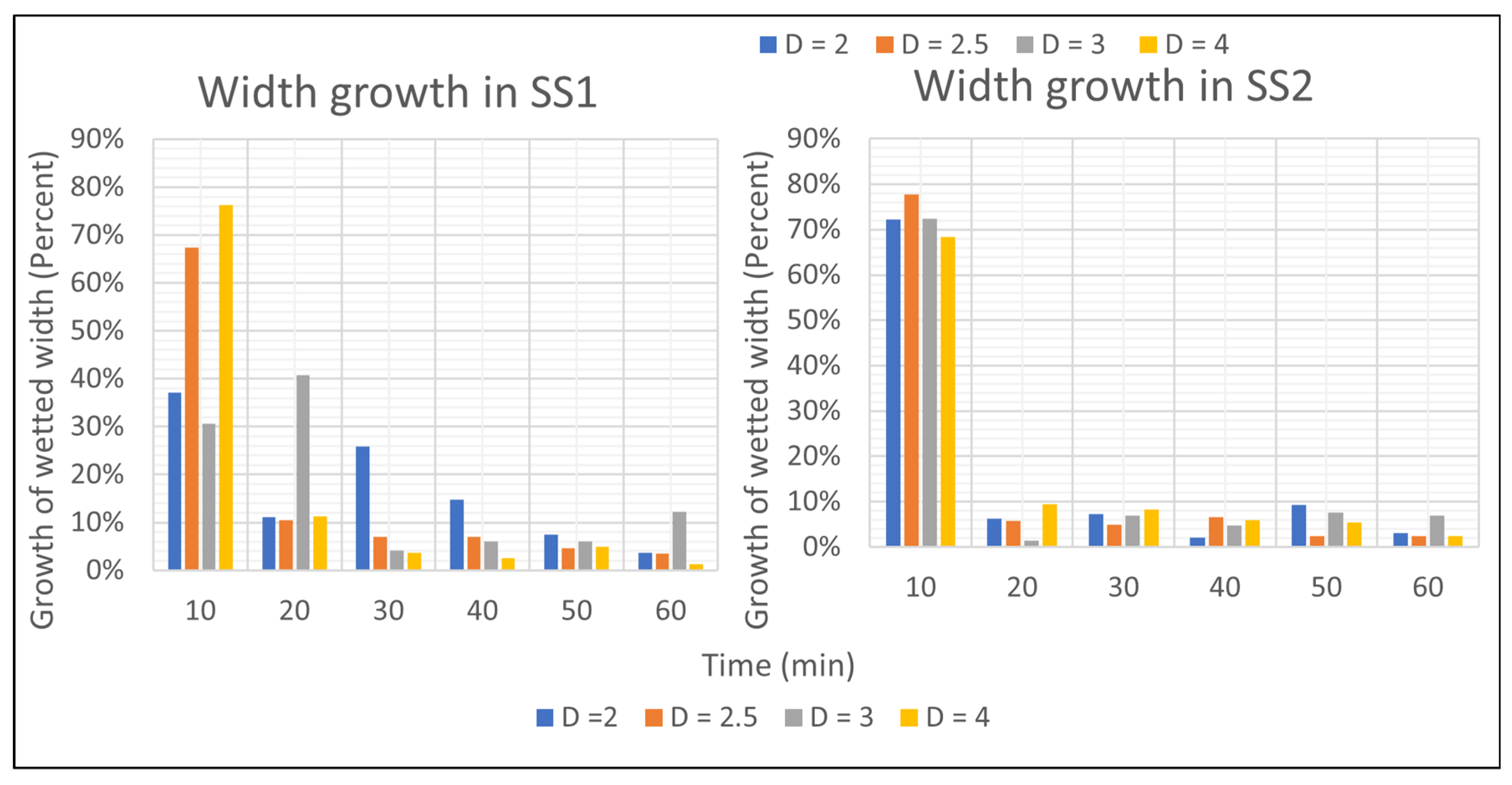
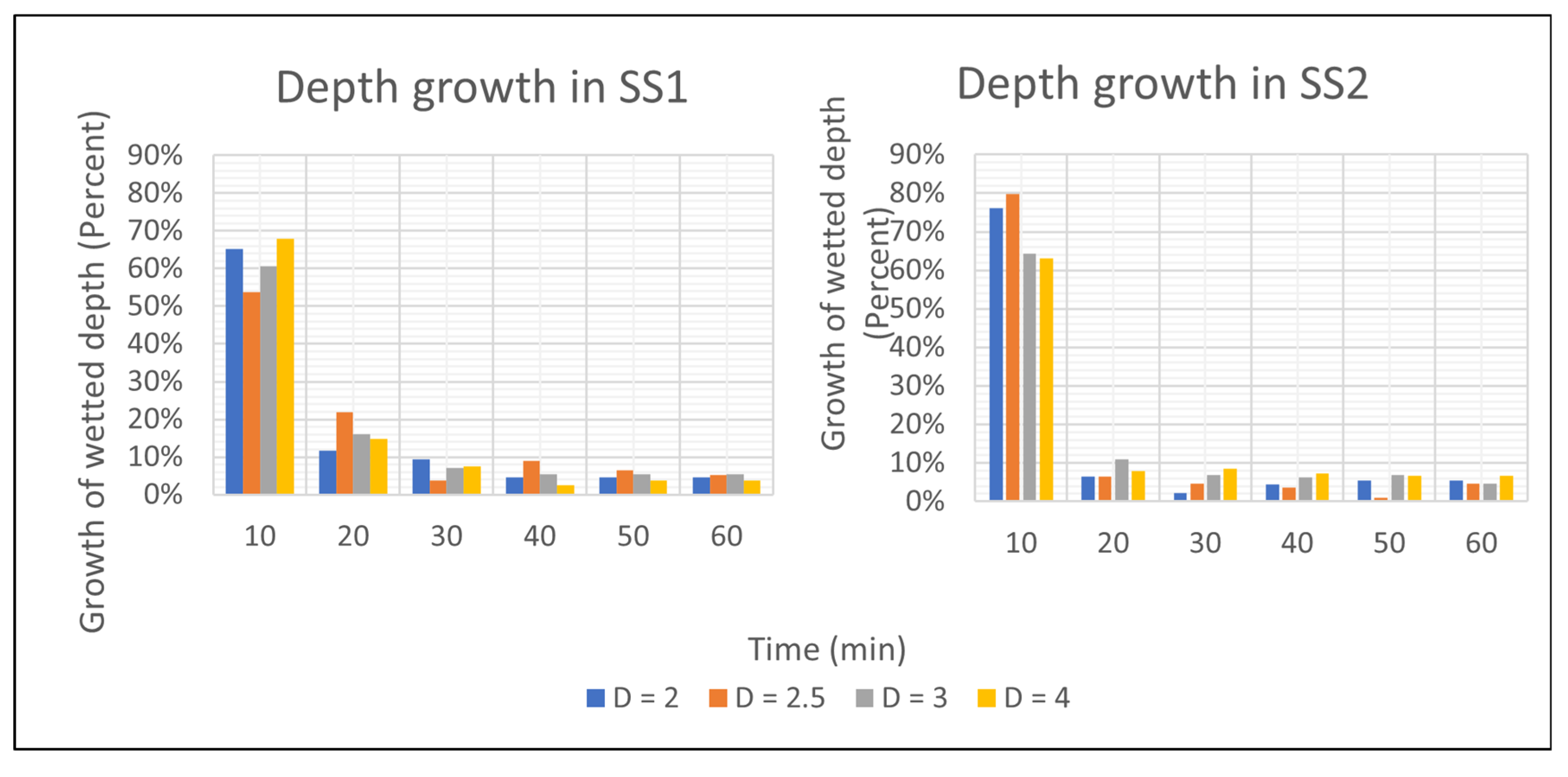
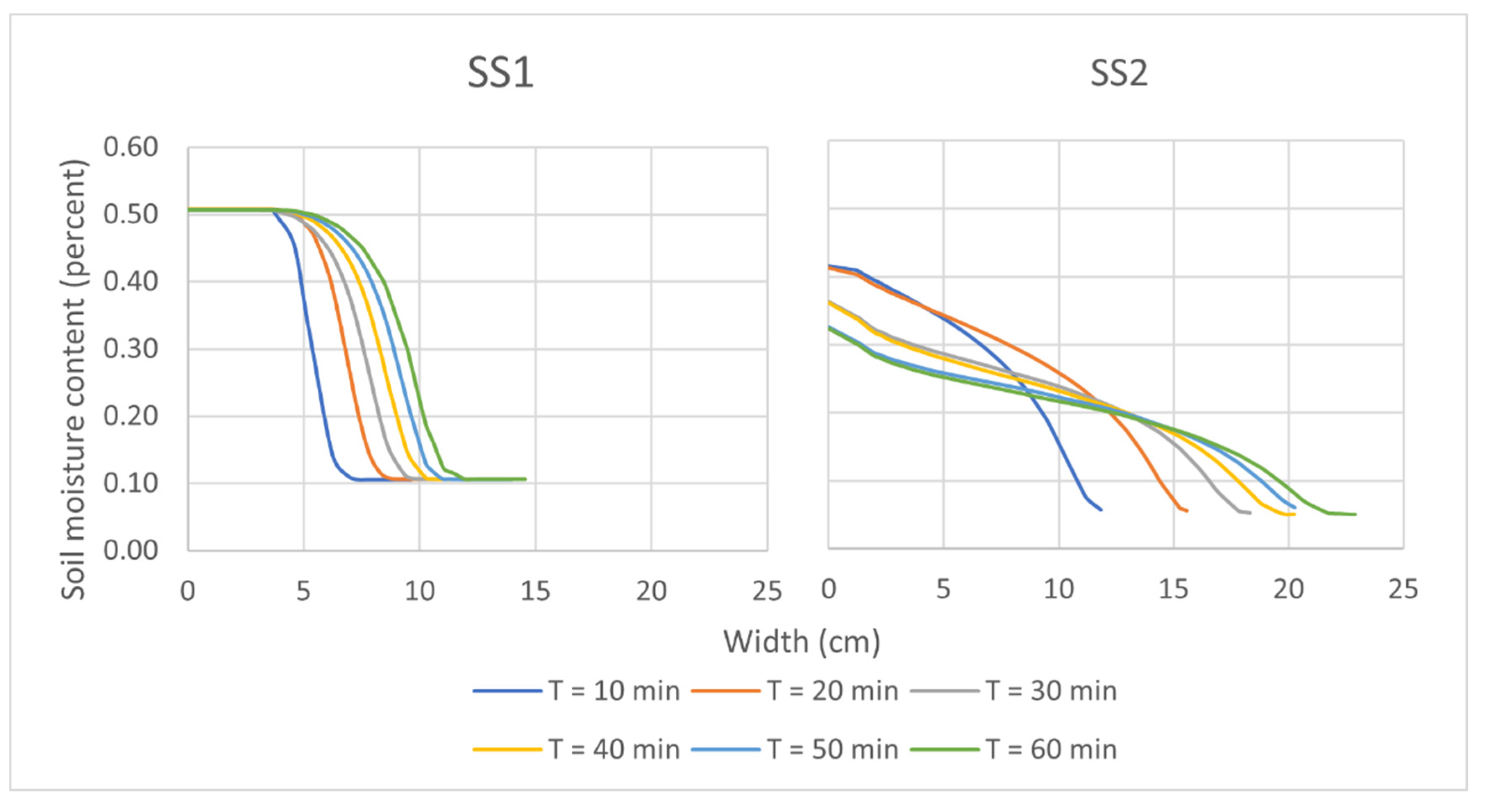
3.1. Experimental Results of BIS Wetting Patterns

BIS infiltration flow rates from the ICPBs have been measured for every 10 min in one-hour of testing duration. Figure 5 illustrates the variation in the infiltration rate for the BIS with time and with different contact areas. In general, the flow rate has been exponentially reduced over time. BIS flow rate in SS2 show higher values than the flow in soil SS1. Since the air bubbles raised from the soil to the ICPB through the contact area, the BIS water flow rate is highly impacted by the hydraulic properties of the soil type and by the opening of the ICPB, that is, the contact area. However, the flow rate was decreased by reducing the diameter of the contact area, and the downward exponential pattern of flow values for the four areas of contact was similar for both soil types. By reducing the area of contact, not only the average flow rate but also the variation of flow has been lowered. Average values of the bubbles flow rate result from using various diameters of contact area into soil SS1 and SS2 are presented in

Table 4. Average infiltration values of bubble flow rate (Lph).

Diameters of the Contact Area (cm)	Soil Type
	SS1	SS2
2	0.296	0.567
2.5	0.183	0.291
3	0.144	0.955
4	0.571	1.004

. The average values show that the flow rate has almost doubled between the two soil types for the same area of contact of diameters 2, 2.5, and 4 cm.

Wetting patterns generated by the bubble flow rates have been traced for each 10 min interval for soil types SS1 and SS2, as shown in Figure 5. The advancement of the wetted area was rapidly increased at the beginning of the test but then decreased towards the end of the test. Differences in the advancement rate during the experiment were due to the differences in air flow rate towards the ICPB from the surrounding soil. For instance, the airflow rate from the surrounding unsaturated soil started with high values, but the airflow rate decreased with the time of the experiment since the surrounding soil became saturated due to water emissions from the ICPB. The early time propagation of the wetting front was nonuniformly distributed, and the majority of flow was downward but, at the later time, the propagation was almost uniform and equal for all directions. The reason for the non-uniformity advancements of the wetted area is that the airflow towards the ICPB is not consistent, which depends upon the air paths in the body of the wetted area created by capillary and gravity actions.

The width and depth of the wetted areas were increased by increasing the diameter of the contact area. The width and depth of wetted fronts in soil type SS1 created by the diameter of the contact area of 2.5 cm were larger than that created by 3 cm due to the initial flow rate of 2.5 cm being higher than 3 cm, which gives a larger amount of water to be distributed. Upward infiltration was not more than 8 cm using the 4 cm diameter of the contact area.

The shape of the wetted patterns were horizontal ellipses in which the major axis lay parallel to the soil surface. Some of the shapes show the effect of soil uniformity, which impacted the smoothness of the ellipse shape. While the centroid of the ellipse, for some cases, started at the center of the contact area and moved downward during the time of the experiment, others started below the center of the contact area from the beginning of the experiments. Figure 6 and Figure 7 show the incremental width and depth of wetting fronts in soil SS1 and SS2, respectively.

Similar to the variation of advancement rates in soil SS1, the advancement rates of the wetting area in soil SS2 rapidly increased at the beginning and slowly decreased toward the end of the test duration. Due to the initial values of flow rate being higher in soil SS2 than the flow rate in soil SS1, the initial advancement rate was higher in soil SS2 than those in soil SS1. Moreover, the wetting patterns in soil SS2 have most of the distribution downward for the initial period of the experiment and equally distributed for the rest of the time. Since the hydraulic conductivity of soil SS2 was higher than soil SS1, the downward advancements were higher in soil SS2 than those in soil SS1.

Likewise, in the wetting patterns in soil SS1, the width and depth of wetting patterns were increased by increasing the diameter of the contact area. Furthermore, the shape of the wetting patterns in SS2 were horizontal ellipses and the major axis lay parallel to the soil surface. Since the pressurized or free flow in sandy soils is affected by gravity more than capillary action, wetting patterns are performed in vertical ellipses in sandy soils. Although the typical shape of wetting patterns in sandy soils is a vertical ellipse [15,38], the observed wetting patterns for BIS are horizontal ellipses with the major axis laid on the horizontal axis since the wetting fronts are controlled by the air–water exchange mechanism. For instance, water application of bubble flows required airflow from the soil to ICPB, which permits a gentle enlargement of wetting fronts for each emission of water. To explain, the enlargements of width were slightly higher than the depth, airflow from the depth of the wetted zone towards the contact area was subjected to resistance to water flow due to gravity, while airflow from the side of the zone was relatively not subjected to this resistance. Therefore, the wetted zone expanded from the sides a little more than in the depth. Thus, the wetted area has formed as a horizontal rather than vertical ellipse.

It can be seen from the Figure 6 and Figure 7 that, in general, the incremental rate of width and depth of flow is highly reduced through time. Moreover, a small area of contact produced a reduction in the size of the wetting pattern, since a smaller area of contact allows lower air–water exchange than the larger area. The size of wetting patterns indicated by width and depth are highly affected by hydraulic conductivity. For instance, wetting patterns in SS1, which have a relatively low hydraulic conductivity, are smaller than those in SS2. Clearly, for all diameters of contact area, the size of wetting fronts created in soil SS1 was smaller than those in soil SS2, because soil SS1 has a smaller value of hydraulic conductivity. The depth and width of the wetting fronts did not exceed 9 cm in soil SS1, while the depth and width of the wetting fronts in soil SS2 did not exceed 16 cm. Figure 8 and Figure 9 show the variation of width and depth respectively of wetted area for SS1 and SS2.

The hydraulic conductivity and the density of soil SS2, which were 62 and 22 percent, respectively, higher than soil SS1 have resulted in average incremental ratios of wetted depth and width of 94 and 178 percent, respectively. The hydraulic conductivity of the soil has a direct effect on the advances of the wetting fronts which produce the air paths in the wetted body of the soil. The density of the soil affects the porosity of the soil which controls the air and water spaces in the water body in the soil. Typical free flow in soil produces an incremental ratio of depth higher than the width, due to the gravity action. On the contrary, the incremental ratio of the depth was lower than that of width in the BIS flow technique.

Maximum wetting advancement happened in the first segment of the time. Growth ratio can be used to represent the enlargement as a percent of the total width and depth in wetting patterns. Figure 10 and Figure 11 show the growth ratio of the wetted area in width and depth during the time of the experiment. The growth ratio of the wetting size is generally reduced over time since, the air bubble flow rate is decreased. For the first ten minute segment time, growth ratios were higher than 50 percent but for the rest of the time segments, they were lower than 10 percent. Different diameters of contact area show the same behavior with some variations due to the variation in bubble flow rate, which produces the variation in the size of wetting patterns. Initial emissions from ICPB have a significant effect on the shape and size of the wetted area. In soil SS1, the average initial growth rate of width and depth of the wetted area were 53 and 62 percent, respectively, while in soil SS2, the average initial growth rate was 73 and 71 percent from the total width and depth.

The soil at initial moisture content has a considerable void which is filled with air. Thus, initial emission of the flow from ICPB are significant observations since the air around the area of contact is available for the air–water exchanging mechanism.

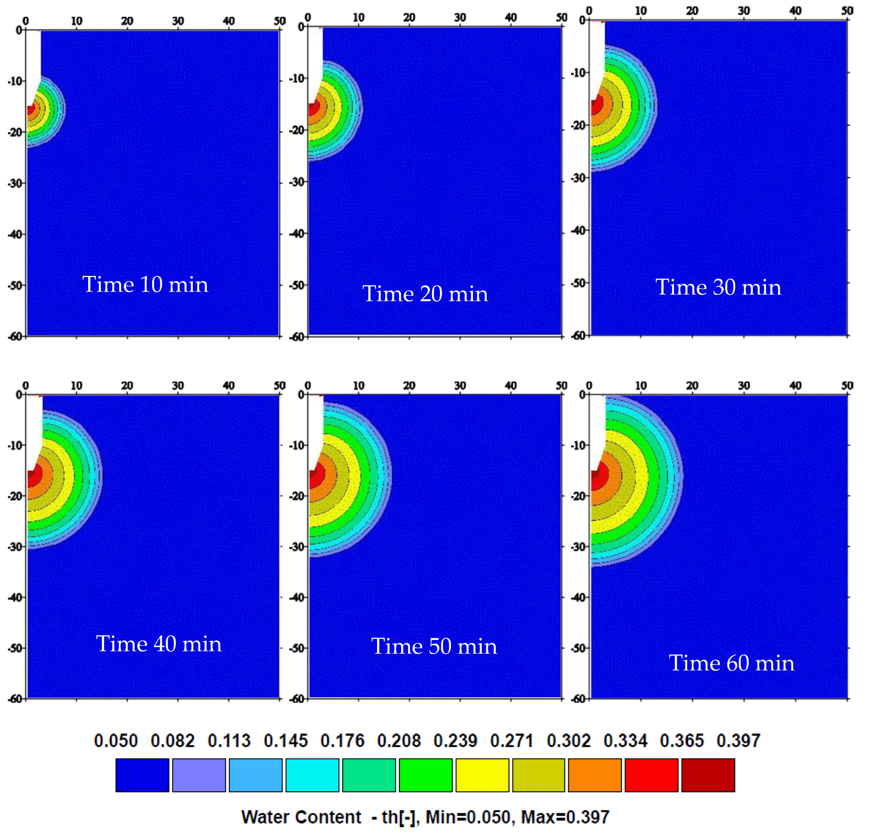
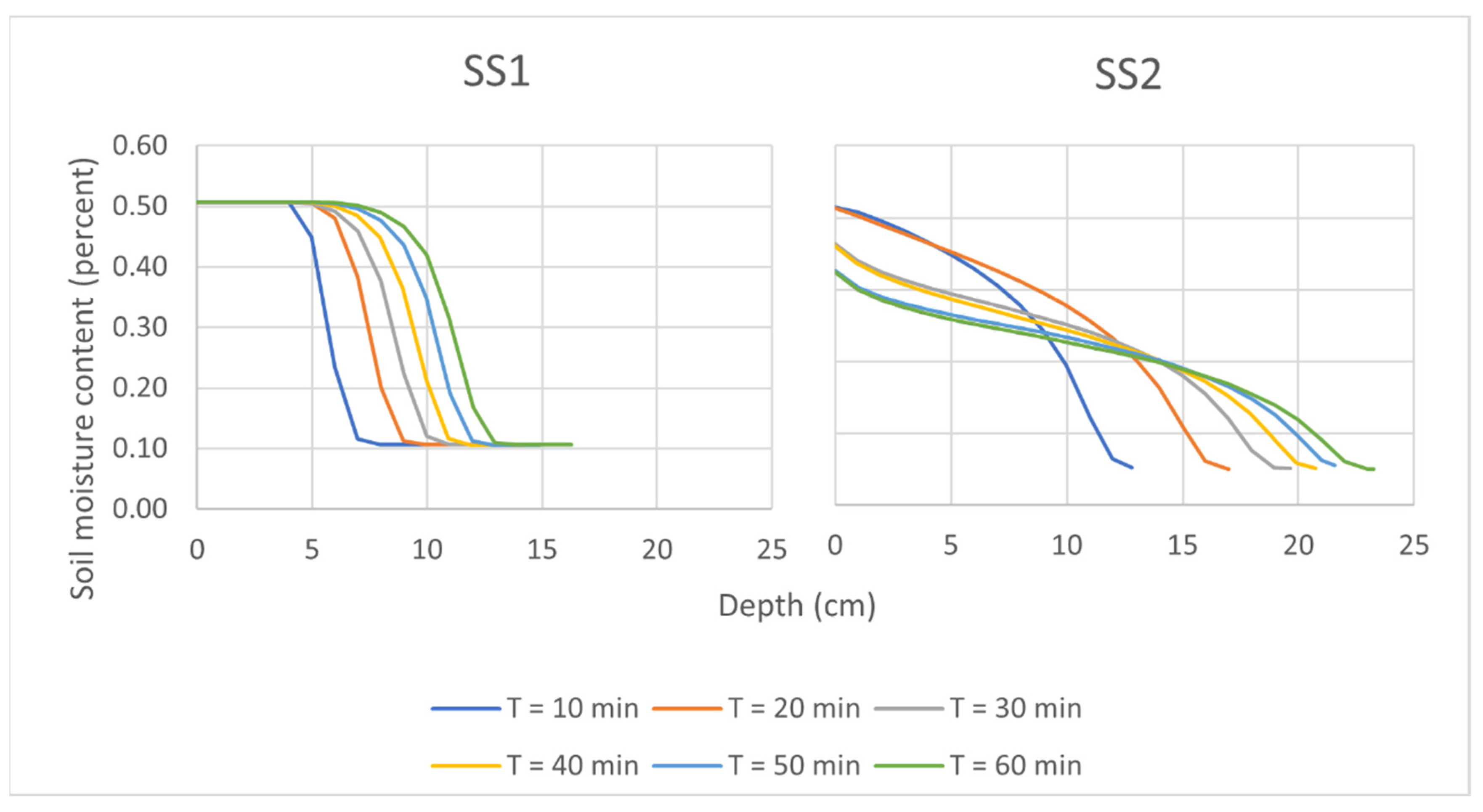
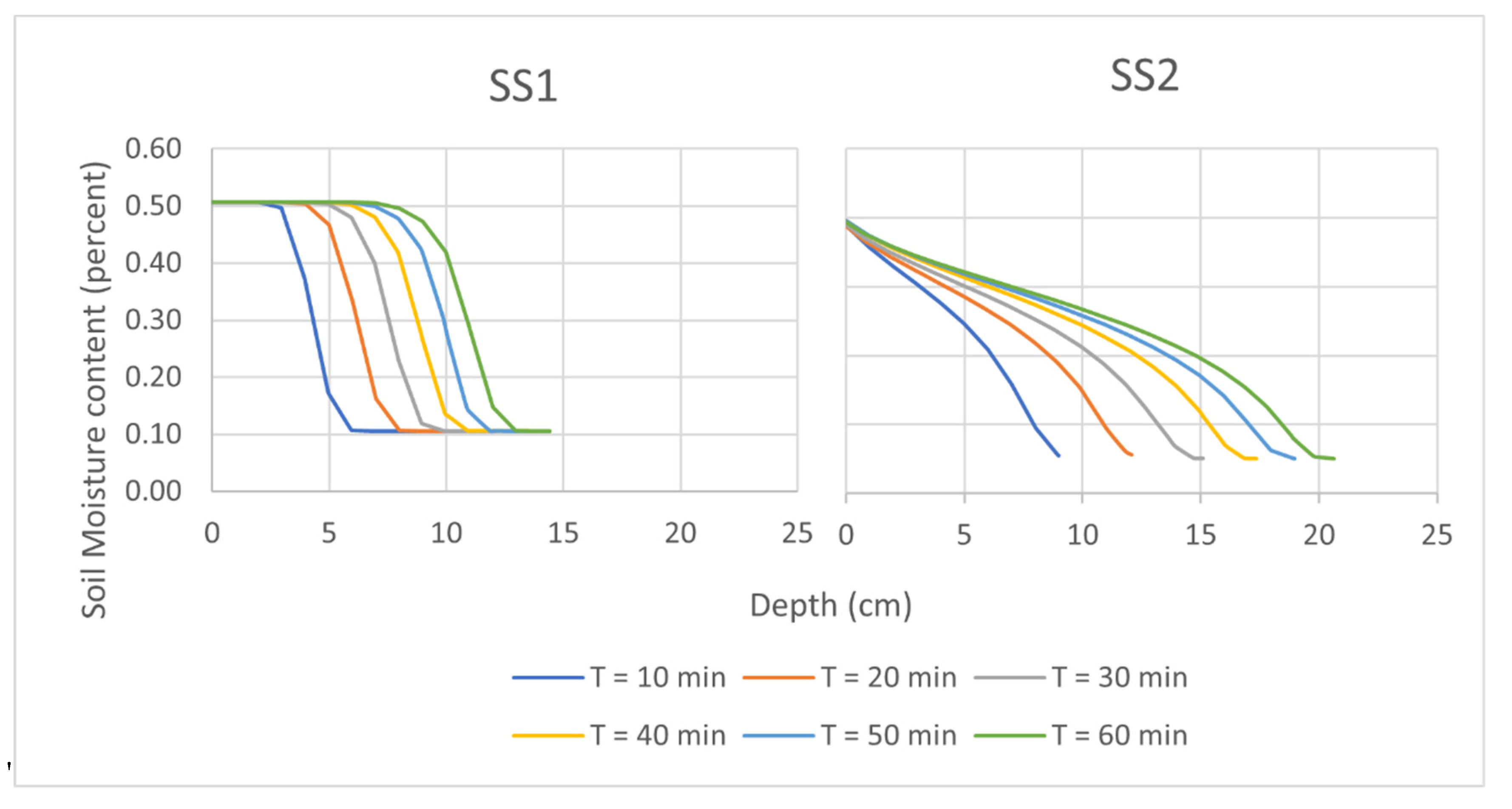
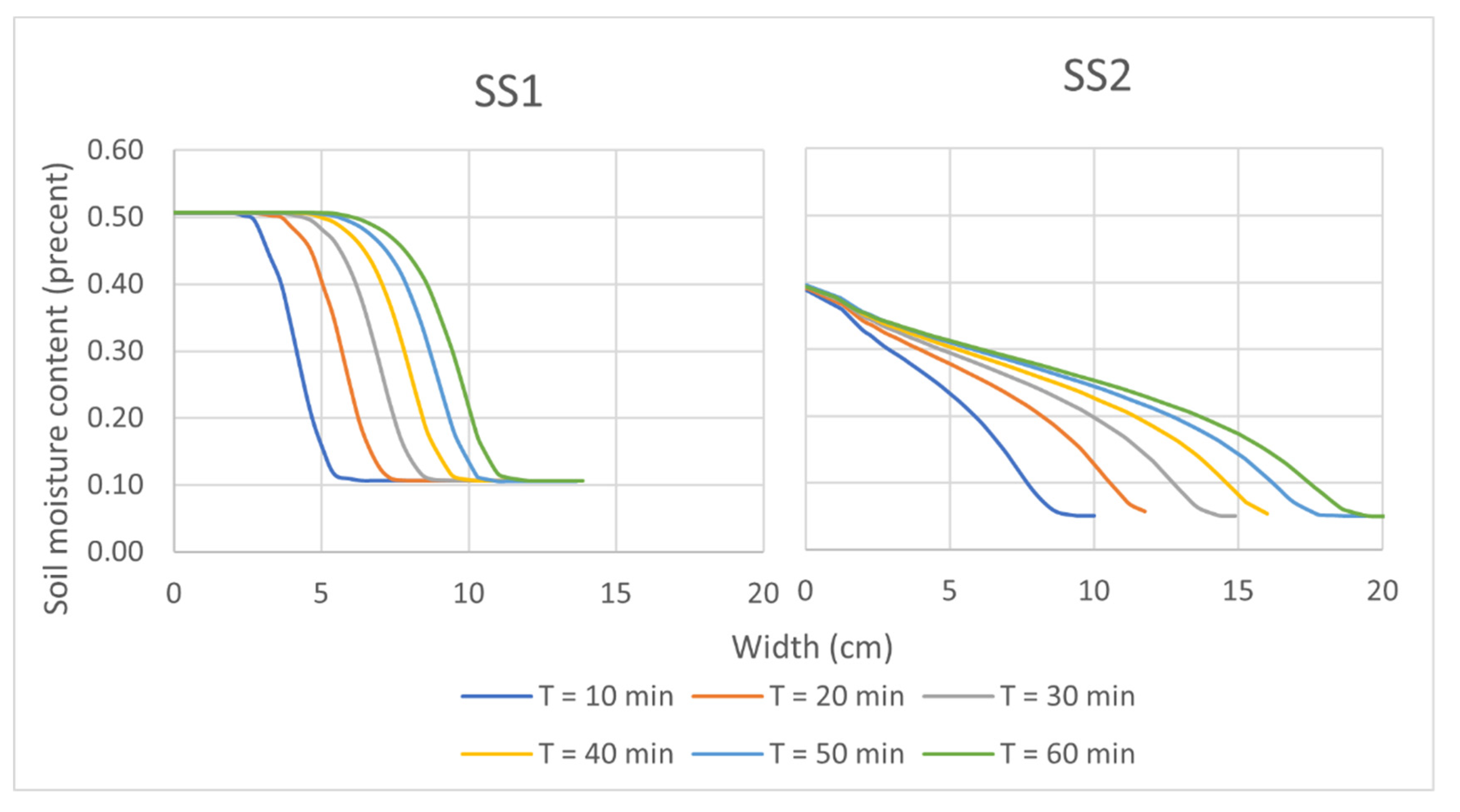
3.2. Results of the 2D HYDRUS Model

The simulations using 2D HYDRUS were conducted under two conditions with flow rates that were varied and constant. For the varied flow condition, the varied flow rate presented in Figure 5 was used while for the constant flow rate condition, the average of that flow rate was used. Moisture content distribution created by constant and varied flow rates was observed and, for example, simulations of constant and varied flow from ICPB with a contact area diameter of 2.5 cm in soil SS2 are given in Figure 12 and Figure 13, respectively. In the case of varied flow rates, the moisture content patterns changed according to the flow rate variation. Due to the high intensity of the bubble flow during the first portion of time, the moisture content distribution increased rapidly. The air bubbles flow significantly reduced with time as the majority of the moisture content was already distributed by the soil, which was when the applied flow became lower than the hydraulic conductivity of the soil.

In the case of constant flow rate conditions, the moisture content patterns were advanced in a consistent shape. When the flow rate used was constant, the intervals of moisture content contour had varied enlargements because the flux emissions were distributed on the perimeter of the wetted area, which increased in size with time.

Sectional profiles in width and depth directions as presented in Figure 14, Figure 15, Figure 16 and Figure 17 have been extracted to show the variation in moisture content in both directions. In general, the slope of moisture distribution in soil SS1 for all cases was steeper than those in soil SS2, since not only the hydraulic conductivity of soil SS1 was lower than soil SS2, but also the field capacity of soil SS1 was higher than that in soil SS2. Because the BIS flow rate was controlled by the water–air exchange, the differences between moisture distribution in width and depth directions were not significant.

In varied flow rate condition, the slopes of moisture distribution along width and depth directions were consistently steep from saturated to residual SMC. This happened because the hydraulic conductivity of the soil was lower than the accumulated flux. For $D_i$ = 2.5 cm, the maximum variation in moisture distribution in soil SS1 was 0.4 cm³/cm³ along 3.8 cm of depth at a time of 10 min. On the other hand, the slope of the moisture distribution profile in soil SS2 in width and depth directions was milder since the applied flux was sometimes lower than the hydraulic conductivity of the soil. Sometimes, the applied flux becomes lower than the hydraulic conductivity of the soil because the applied flux depends on the airflow received by ICPB, which is gradually reduced according to the air–water exchange mechanism. Moreover, since the intensity of flow is reduced with time, the latest moisture distribution patterns become flatter than the earliest patterns. Thus, some of the latest patterns of moisture content variation had started lower than the saturated moisture content. The flatter variation in the moisture distribution pattern of case 2 was 0.3 along 23 cm in the depth direction at a time of 60 min.

In constant average flow rate conditions, variations of moisture content in SS2 were more regular than those of varied flow since the inflow was steady. The average flow rates used in case 2 were 0.183 and 0.291 Lph for SS1 and SS2, respectively. The moisture variation became flatter with time since the area of distribution became larger. In contrast with the patterns of varied flow rate, moisture distribution in soil SS2 produced from constant average flow rate at the beginning and end of the test duration were started from the same point of the saturated zone at 0.415 cm³/cm³ since the flow intensity is constant and has a higher value than the hydraulic conductivity of the soil.

Sharp and non-sharp wetting fronts have been intercepted to show the distance representation of the wetting front in the moisture content distribution. The interception of the sharp and non-sharp wetting fronts for all cases using actual varied and average applied discharge are shown in Figure 18 and Figure 19.

In the case of soil SS1, results of interception of sharp and non-sharp wetting fronts using varied and the constant average bubbles flow showed that the average intercepted soil moisture content, SMC, was 0.46 and 0.44 percent, respectively. Using various and constant bubble flow rates, more than 75% of the intercepted points of SMC were above the average of SMC. Because the variation of moisture content in soil A has a steep profile as shown in Figure 14, Figure 15, Figure 16 and Figure 17, most of the intercepted SMC were near the saturated state. In conclusion, the properties of soil SS1 may indicate that the sharp wetting front can be predicted to be near the saturated zone of the soil.

Intercepted SMC for soil SS2, shows that the average intercepted SMC for sharp and non-sharp wetting fronts using varied and average bubble flow conditions were 0.3 and 0.26 percent, respectively. For actual varied conditions, 60 percent of the intercepted SMC were above the average while, for a constant average flow rate, 58 percent were above average. Because the variation of moisture content in SS2 has a flat profile as shown in Figure 14, Figure 15, Figure 16 and Figure 17, the intercepted SMC were distributed in a wide range of moisture content. This indicates that the sharp wetting fronts in soil SS2 can be predicted to be in the range between the saturated state and the average intercepted SMC. The distribution of the interception between sharp and non-sharp wetting fronts is highly dependent on the soil type.

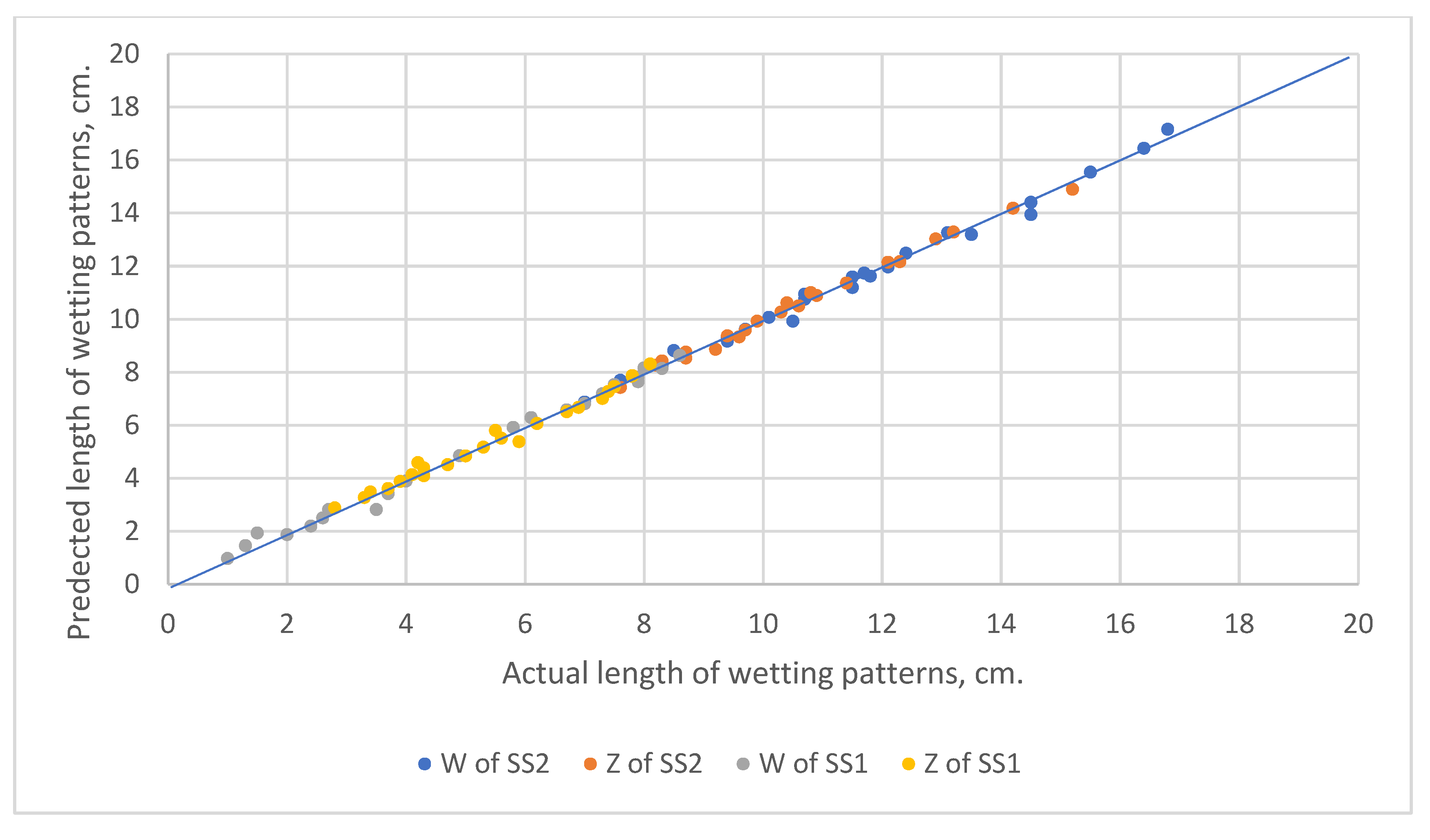
3.3. Statistical Analysis

Based on experimental and numerical simulation results, statistical multiple regression models were derived using R-Studio software to predict the average BIS flow rate and the width and depth of the wetting fronts. The independent variables used to generate this statistical model were the diameter of the contact area and the hydraulic conductivity of the soil.

For constant ${\beta }_o$, ${\beta }_1$, and ${\beta }_2$, in the bubble flow rate equation (Equation (4)) the statistical model’s parameters were −1.07, 0.22, and 0.613, respectively. This model had a multiple R-squared of 0.69, a correlation coefficient of 0.836, and a root mean square of error RMSE of 0.17. A statistical t-test was performed to check that the null hypothesis of the mean difference was zero. Results of the t-test show that the value of t statistics was 0.00025 and the t-critical two-tail was ±2.36 which means the null hypothesis is accepted, meaning that there are no significant differences between the obtained and the predicted average bubble flow rates. In addition, the multicollinearity of the independent variables has been evaluated using the variance inflation factor, VIF. Values of VIF for both the diameter of the contact area and the soil hydraulic conductivity were 1, which means there is no relation between these variables. In conclusion, this model can be efficiently used to predict the average bubble flow rate.

The equivalent radius formula introduced by Ben-Asher (Equation (1)) was used to create a set of equations to predict the width and depth of wetting fronts by introducing modification factors A, B, C and D (Equations (2) and (4)); the factors were determined using linear regression analysis. The parameters of these equations and the coefficient of determination, R², for each equation are presented in

Table 5. Parameters and the coefficient of determination resultant from regression analysis between the equivalent radius and the actual size of the wetting pattern.

K	Diameters	Width Parameters (w)			Depth Parameters (z)
		C	D	R2	A	B	R2
SS1	2	0.50	0.11	0.96	2.49	0.09	0.98
	2.5	5.23	0.19	0.98	3.75	0.23	0.94
	3	1.06	0.23	0.89	2.87	0.16	0.98
	4	5.76	0.09	0.95	5.10	0.12	0.94
SS2	2	6.06	0.12	0.96	6.20	0.09	0.96
	2.5	8.48	0.15	0.99	8.10	0.12	0.98
	3	8.90	0.14	0.95	7.26	0.16	0.99
	4	9.93	0.17	0.99	7.67	0.17	0.99

. Also, a comparison of the predicted and actual size of wetting patterns can be presented in Figure 20.

The BIS flow rate was tested in 2D HYDRUS using varied and average flow rates to produce non-sharp wetting patterns. The results of the non-sharp wetting patterns were tested using a two-tail paired t-test to check the hypotheses if there were no significant differences between the result of using varied and average bubbles flow rates. T statistics were −1.464 and −3.59, and t critical was ±2.01 for both tests. Thus, the results of the test accept the null hypothesis for SS1 and reject it for SS2 which means there are no significant differences between using varied and average bubble flow rates for SS1, but there are significant differences for SS2. Therefore, the average bubble flow rate can be used to simulate the flow in 2D HYDRUS for SS1 but cannot be used for SS2.

4. Conclusions

The concept governing the BIS is presented in this paper, as well as laboratory measurements of wetting fronts patterns created by a specially designed air–water bubbles emitter, numerical simulations of the BIS with non-sharp wetting fronts, and a statistical model to predict the size of wetting patterns for the bubbles irrigation system.

The experiments and the numerical simulations show that the soil type and the area of contact have a high impact on the bubbles flow rate and on the shape and size of wetting patterns. In addition, most of the size of the wetting pattern is produced in the first portion of time, which presents the impact of the bubbles flow technique. In the first portion of time, more than 50 percent of width and depth have been performed in SS1 and more than 70 percent have been performed in SS2.

Bubbles flow in the soil can be represented in 2D HYDRUS using the actual varied flow rate. Unlike the actual varied flow, the average constant bubbles flow rate can be used to simulate the flow in 2D HYDRUS for SS1 but cannot be used for SS2 since there are significant differences with the obtained results. Moreover, using a constant head in 2D HYDRUS was not representative [39] since the constant head pressurized the flow in soil, unlike the bubble technique.

Statistical tests show that the average flow rate can be predicted efficiently to represent the bubbles flow. In addition, 2D HYDRUS can be used accurately to locate the sharp wetting front using a suitable reduction ratio. The sharp wetting fronts in SS2 can be predicted to be in the range between the saturated state and the average intercepted SMC. The distribution of the interception between sharp and non-sharp wetting fronts is highly dependent on the soil type.

The findings from this study provide insight on the workability and effectiveness of BIS in controlling the growth of the wetting patterns in subsurface irrigation. BIS adopts a unique air–water exchange technique to provide control on the applied amount of irrigation water. The amount of water supply is controlled based on the soil moisture deficit, i.e., based on the actual water consumption by the plants. Moreover, reliable equations for estimating the BIS wetting dimensions using simulated non-sharp wetting fronts have been successfully developed. Further investigation on the design criteria for the bubbles subsurface irrigation system and its practicality are ongoing.

References

1. Chenafi, A.; Monney, P.; Arrigoni, E.; Boudoukha, A.; Carlen, C. Influence of irrigation strategies on productivity, fruit quality and soil-plant water status of subsurface drip-irrigated apple trees. Fruits 2016, 71, 69–78. [Google Scholar] [CrossRef]
2. Heard, J.; Porker, M.; Armstrong, D.; Finger, L.; Ho, C.; Wales, W.; Malcolm, B. The economics of subsurface drip irrigation on perennial pastures and fodder production in Australia. Agric. Water Manag. 2012, 111, 68–78. [Google Scholar] [CrossRef]
3. Wang, Y.P.; Zhang, L.S.; Mu, Y.; Liu, W.H.; Guo, F.X.; Chang, T.R. Effect of A Root-Zone Injection Irrigation Method on Water Productivity and Apple Production in A Semi-Arid Region In North-Western China. Irrig. Drain. 2020, 69, 74–85. [Google Scholar] [CrossRef]
4. Yao, W.W.; Ma, X.Y.; Li, J.; Parkes, M. Simulation of point source wetting pattern of subsurface drip irrigation. Irrig. Sci. 2011, 29, 331–339. [Google Scholar] [CrossRef]
5. Elmaloglou, S.; Diamantopoulos, E. Simulation of soil water dynamics under subsurface drip irrigation from line sources. Agric. Water Manag. 2009, 96, 1587–1595. [Google Scholar] [CrossRef]
6. Charlesworth, P.B.; Muirhead, W.A. Crop establishment using subsurface drip irrigation: A comparison of point and area sources. Irrig. Sci. 2003, 22, 171–176. [Google Scholar] [CrossRef]
7. Philip, J. What happens near a quasi-linear point source? Water Resour. Res. 1992, 28, 47–52. [Google Scholar] [CrossRef]
8. Warrick, A. Comment on “What happens near a quasi-linear point source?” by JR Philip. Water Resour. Res. 1993, 29, 3299–3300. [Google Scholar] [CrossRef]
9. Shani, U.; Xue, S.; Gordin-Katz, R.; Warrick, A. Soil-limiting flow from subsurface emitters. I: Pressure measurements. J. Irrig. Drain. Eng. 1996, 122, 291–295. [Google Scholar] [CrossRef]
10. Alrubaye, Y.L.; Yusuf, B. Former and Current Trend in Subsurface Irrigation Systems. Pertanika J. Sci. Technol. 2021, 29, 1–30. [Google Scholar] [CrossRef]
11. Alrubaye, Y.L.; Yusuf, B.; Hamad, S.N. Development of a Self-regulated Bubble Irrigation System to Control the Size and Shape of Wetting Fronts. Pertanika J. Sci. Technol. 2020, 28, 1297–1313. [Google Scholar] [CrossRef]
12. Parkin, G.W.; Gardner, W.H.; Auerswald, K.; Bouma, J.; Chesworth, W.; Morel-Seytoux, H.J. Wetting Front. In Encyclopedia of Soil Science; Chesworth, W., Ed.; Springer: Dordrecht, The Netherlands, 2008; pp. 830–835. [Google Scholar]
13. Lu, N.; Likos, W. Unsaturated Soil Mechanics; John Wiley & Sons Inc.: Hoboken, NJ, USA, 2004. [Google Scholar]
14. Philip, J.R. Theory of infiltration. In Advances in Hydroscience; Elsevier: Amsterdam, The Netherlands, 1969; Volume 5, pp. 215–296. [Google Scholar]
15. Angelakis, A.N.; Rolston, D.E.; Kadir, T.N.; Scott, V.H. Soil-water distribution under trickle source. J. Irrig. Drain. Eng. 1993, 119, 484–500. [Google Scholar] [CrossRef]
16. Chu, S.-T. Green-Ampt analysis of wetting patterns for surface emitters. J. Irrig. Drain. Eng. 1994, 120, 414–421. [Google Scholar] [CrossRef]
17. Green, W.H.; Ampt, G. Studies on Soil Phyics. J. Agric. Sci. 1911, 4, 1–24. [Google Scholar] [CrossRef]
18. Richards, L.A. Capillary conduction of liquids through porous mediums. Physics 1931, 1, 318–333. [Google Scholar] [CrossRef]
19. Ben-Asher, J.; Charach, C.; Zemel, A. Infiltration and water extraction from trickle irrigation source: The effective hemisphere model. Soil Sci. Soc. Am. J. 1986, 50, 882–887. [Google Scholar] [CrossRef]
20. Abid, H.N.; Abid, M.B. Predicting Wetting Patterns in Soil from a Single Subsurface Drip Irrigation System. J. Eng. 2019, 25, 41–53. [Google Scholar] [CrossRef]
21. Ali, S.; Ghosh, N.C. Methodology for the estimation of wetting front length and potential recharge under variable depth of ponding. J. Irrig. Drain. Eng. 2015, 142, 04015027. [Google Scholar] [CrossRef]
22. Dawood, I.A.; Hamad, S.N. Movement of Irrigation Water in Soil from a Surface Emitter. J. Eng. 2016, 22, 103–114. [Google Scholar]
23. Fan, W.; Li, G. Effect of soil properties on Hydraulic characteristics under subsurface drip irrigation. IOP Conf. Ser. Earth Environ. Sci. 2018, 121, 052042. [Google Scholar] [CrossRef]
24. Ren, C.; Zhao, Y.; Dan, B.; Wang, J.; Gong, J.; He, G. Lateral hydraulic performance of subsurface drip irrigation based on spatial variability of soil: Experiment. Agric. Water Manag. 2018, 204, 118–125. [Google Scholar] [CrossRef]
25. Fan, Y.; Huang, N.; Gong, J.; Shao, X.; Zhang, J.; Zhao, T. A simplified infiltration model for predicting cumulative infiltration during vertical line source irrigation. Water 2018, 10, 89. [Google Scholar] [CrossRef]
26. Fan, Y.-W.; Huang, N.; Zhang, J.; Zhao, T. Simulation of soil wetting pattern of vertical moistube-irrigation. Water 2018, 10, 601. [Google Scholar] [CrossRef]
27. Cai, Y.; Wu, P.; Zhang, L.; Zhu, D.; Chen, J.; Wu, S.; Zhao, X. Simulation of soil water movement under subsurface irrigation with porous ceramic emitter. Agric. Water Manag. 2017, 192, 244–256. [Google Scholar] [CrossRef]
28. Cai, Y.; Wu, P.; Zhang, L.; Zhu, D.; Wu, S.; Zhao, X.; Chen, J.; Dong, Z. Prediction of flow characteristics and risk assessment of deep percolation by ceramic emitters in loam. J. Hydrol. 2018, 566, 901–909. [Google Scholar] [CrossRef]
29. Cai, Y.; Zhao, X.; Wu, P.; Zhang, L.; Zhu, D.; Chen, J. Effect of Soil Texture on Water Movement of Porous Ceramic Emitters: A Simulation Study. Water 2019, 11, 22. [Google Scholar] [CrossRef]
30. Cai, Y.; Zhao, X.; Wu, P.; Zhang, L.; Zhu, D.; Chen, J.; Lin, L. Ceramic patch type subsurface drip irrigation line: Construction and hydraulic properties. Biosyst. Eng. 2019, 182, 29–37. [Google Scholar] [CrossRef]
31. Lima, V.; Keitel, C.; Sutton, B.; Leslie, G. Improved water management using subsurface membrane irrigation during cultivation of Phaseolus vulgaris. Agric. Water Manag. 2019, 223, 105730. [Google Scholar] [CrossRef]
32. Saefuddin, R.; Saito, H.; Šimůnek, J. Experimental and numerical evaluation of a ring-shaped emitter for subsurface irrigation. Agric. Water Manag. 2019, 211, 111–122. [Google Scholar] [CrossRef]
33. Malek, K.; Peters, R.T. Wetting pattern models for drip irrigation: New empirical model. J. Irrig. Drain. Eng. 2011, 137, 530–536. [Google Scholar] [CrossRef]
34. Gao, Y.; Li, Z.; Sun, D.A.; Yu, H. A simple method for predicting the hydraulic properties of unsaturated soils with different void ratios. Soil Tillage Res. 2021, 209, 104913. [Google Scholar] [CrossRef]
35. Van Genuchten, M.T. A closed-form equation for predicting the hydraulic conductivity of unsaturated soils 1. Soil Sci. Soc. Am. J. 1980, 44, 892–898. [Google Scholar] [CrossRef]
36. DiCarlo, D.A. Quantitative network model predictions of saturation behind infiltration fronts and comparison with experiments. Water Resour. Res. 2006, 42, 9. [Google Scholar] [CrossRef]
37. Kisi, O.; Khosravinia, P.; Heddam, S.; Karimi, B.; Karimi, N. Modeling wetting front redistribution of drip irrigation systems using a new machine learning method: Adaptive neuro-fuzzy system improved by hybrid particle swarm optimization–Gravity search algorithm. Agric. Water Manag. 2021, 256, 107067. [Google Scholar] [CrossRef]
38. Lazarovitch, N.; Warrick, A.; Furman, A.; Simunek, J. Subsurface water distribution from drip irrigation described by moment analyses. Vadose Zone J. 2007, 6, 116–123. [Google Scholar] [CrossRef] [Green Version]
39. AL-Sammak, A.S. Wetting Pattern Characteristics of Unsaturated Flow Created by Free and Bubbles Subsurface Sources. Master Thesis, Universiti Purta Malaysia, Shaden, Malaysia, 2021. [Google Scholar]
Figure 1. The setup model of laboratory experiments for tracing wetting patterns created by bubbles. Source using ICPB in the soil profile.
Sustainability 14 11492 g001
Figure 2. Schematic of the wetting front varies with the time generated by ICPB according to the equivalent radius.
Sustainability 14 11492 g002
Figure 3. Schematic of moisture content distribution in the length of flow for sharp and non-sharp wetting fronts.
Sustainability 14 11492 g003
Figure 4. Boundary conditions and finite element mesh created for HYDRUS-2D simulations are shown in the domain geometry.
Sustainability 14 11492 g004
Figure 5. Variation of BIS flow rate for SS1 and SS2.
Sustainability 14 11492 g005
Figure 6. Size and shape of wetting patterns created by BIS flow rate in SS1.
Sustainability 14 11492 g006
Figure 7. Size and shape of wetting patterns created by the bubbles flow rate in SS2.
Sustainability 14 11492 g007
Figure 8. Width of wetted area for SS1 and SS2 throughout the test duration.
Sustainability 14 11492 g008
Figure 9. Depth of wetted area for SS1 and SS2 throughout the test duration.
Sustainability 14 11492 g009
Figure 10. Growth ratio of wetted width in soil SS1 and SS2 for diverse contact areas.
Sustainability 14 11492 g010
Figure 11. Growth ratio of wetted depth in soil SS1 and SS2 for diverse contact areas.
Sustainability 14 11492 g011
Figure 12. Distribution of soil moisture content for varied flow from the ICPB of the contact area. D = 2.5 cm in soil type SS2.
Sustainability 14 11492 g012
Figure 13. Distribution of soil moisture content resultant of constant flow from the ICPB of the contact area. D = 2.5 cm in soil type SS2.
Sustainability 14 11492 g013
Figure 14. Variation of moisture content in width direction for case 2 using actual varied flow rate.
Sustainability 14 11492 g014
Figure 15. Variation of moisture content in depth direction for case 2 using actual varied flow rate.
Sustainability 14 11492 g015
Figure 16. Variation of moisture content in width direction for case 2 using constant average flow rate.
Sustainability 14 11492 g016
Figure 17. Variation of moisture content in depth direction for case 2 using constant average flow rate.
Sustainability 14 11492 g017
Figure 18. Interception of sharp wetting fronts in the distribution of moisture content for soil SS1 using actual varied and constant flow rate.
Sustainability 14 11492 g018
Figure 19. Interception of sharp wetting fronts in the distribution of moisture content for soil SS2 using actual varied and constant flow rate.
Sustainability 14 11492 g019
Figure 20. Comparison of the predicted and actual size of wetting patterns.
Sustainability 14 11492 g020