Energy-Saving Manufacturing System Design with Two Geometric Machines

Abstract

In recent years, due to increasing energy costs and deteriorating environmental conditions, manufacturing enterprises have become more concerned with energy efficiency. This paper is dedicated to minimizing energy consumption while maintaining the target productivity of a two-machine geometric serial line. To address this problem, we propose a nonlinear model under productivity constraints, where the system energy consumption consists of three components, namely, the setup, the idle, and the normal working energy consumption. By analyzing the properties of the energy consumption function, a new heuristic method, i.e., the energy consumption minimization (ECM) algorithm, is proposed to obtain the optimal solution. In addition, we extend the formulation to further investigate the energy saving problem with varied buffer capacities and propose an energy-saving (ES) algorithm to solve it based on the problem structure. Furthermore, the effectiveness of the algorithms is verified by designing numerical examples, and the effects of energy consumption parameters, buffer capacity, target productivity, and breakdown probabilities on the total energy consumption and optimal solution are presented.

1. Introduction

Nowadays, the manufacturing industry is facing the problem of reducing energy consumption and greenhouse gas emissions due to increasing energy costs and environmental concerns. China’s industrial energy consumption accounts for about $65\%$ of the total energy consumption in society, and there is a large amount of energy consumption in many manufacturing processes, such as heating, painting, casting, and welding. Kolta [1] and Galitsky and Worrell [2] indicate that the assembly and paint shops of automotive assembly plants are typically energy-intensive mass production manufacturing systems. However, the energy storage of available energy can no longer meet the needs of national development. Thus, there is no doubt that improving energy efficiency will be a continuous focus of the international community.

Due to the complexity of production systems, most studies are devoted to the analysis of their steady-state behavior. Additionally, in recent years, it has been recognized that transient analysis is one of the important directions for production systems, and the transient performance of production lines containing geometric reliability machines has been studied. However, the production rate and energy consumption indicators of the geometric series production lines are analyzed independently, without any connection between the two. Production rate analysis is usually performed ignoring energy consumption or assuming it as constant. To the best of our knowledge, only a limited amount of literature consider both the production rate and the energy consumption in geometric production lines, despite the close relationship between the energy consumption and productivity. Therefore, an integrated model incorporating the production rate and the energy consumption is considered in this paper to achieve the aim of reduction of energy consumption in geometric serial production lines under the production rate constraint.

To contribute to the literature on the energy-sensitive geometric production lines, the main contributions of this paper are hereby threefold. First, the optimzation model to minimize the total system energy consumption in a two-machine geometric machine line with a multi-state energy consumption rate while satisfying the constraint of the production rate is formulated. Specifically, the energy consumption of the machine during setup, idle and normal states are considered. Then, the problems taking account of two sets of decision variables, i.e., the machine efficiencies of both machines and the buffer capacity together with the efficiency of the second machine, are considered. The optimality conditions are explored for the two problems, and two tailored algorithms are designed to handle them by analyzing the problem features. Finally, discrete-time simulations are performed to verify the effectiveness of the proposed algorithms. The numerical results demonstrate that the gaps between the algorithms and simulations are within 5.83%.

The remainder of this paper is organized as follows. The literature review is discussed in Section 2. Section 3 introduces the system model and problem formulation of the two-machine geometric line. In Section 4, the problem properties are discussed and the algorithm are proposed to solve the problems optimally. Then, the numerical and sensitivity analysis are performed with simulation results listed in Section 5. Finally, conclusions are presented in Section 6.

2. Literature Review

Production system optimization has received tremendous research attention over the past several decades [3,4,5,6]. The main fields of interest are productivity analysis [7,8,9], quality improvement [10], work-in-process optimization [11], lead time reduction [12], and customer demand satisfaction [13]. Among these studies, maintaining and improving the productivity of the production systems based on the throughput analysis is one of the mainstream topics. To better understand this theory, readers are encouraged to read the famous book Production System Engineering written by Li and Meerkov [5]. In the meantime, it is worth noticing that most of the above studies fail to take into account the energy consumption in the analysis, despite their inherent interdependency. In practice, reducing energy consumption often leads directly to a loss of productivity. Additionally, energy saving becomes a vital concern due to the skyrocketing energy cost and the global climate change in recent years [14,15]. Therefore, we can no longer ignore energy consumption when analyzing the production system performance. To that end, the very target of the present paper is to improve energy savings in the production system.

Many studies have highlighted adopting strategies to control idle machines as an effective measure to save energy. Li and Sun [16] constructed an analytical model of a manufacturing system with multiple machines and buffers and dynamically controlled the system state to achieve the reduction of energy consumption. An on-off control policy to switch off the idle machines in a pallet-constrained flow shop was developed by Mashaei and Lennartson [17]. Cui et al. [18] introduced a control method based on the N-policy and formulated an energy-efficient control model to reduce the system energy consumption. In particular, Frigerio and Matta [19] proposed a new three-parameter control policy based on both buffer and time information, called the TNT-policy, which can save significant energy. Renna and Materi [20] developed switch-off policies based on workload approaches to reduce energy waste in job shop production systems. These papers introduce control strategies to reduce the energy consumption based on machine and workload states, but do not consider the effect of productivity. In addition to the above control strategies, the WIP-based control policy is also an effective method. For instance, Jia et al. [21] adopted the buffer-based feedback policy to switch on/off machines in a Bernoulli serial production line and developed analytical methods to measure the system performance. Although system performances such as productivity, WIP and energy consumption are obtained, the relationships among these indices, for instance, the relationship between the productivity and the energy consumption, are not explored. Several other forms of control strategies are also investigated in the literature, e.g., by Li et al. [22], who introduced a state-based model to dynamically control production systems in order to reduce the energy consumption and maintain target productivity. The control model they propose is a Markov decision process, where the optimal control strategy is obtained by systematically analyzing the energy consumption and production. Instead of deriving a mathematical relationship between the productivity and the energy consumption, a Q-learning algorithm is applied to search for the optimal energy control policy.

At the same time, scheduling is usually applied to energy saving. Chen et al. [23] used transient analysis to study energy saving in serial production lines containing Bernoulli machines and finite buffers and proposed a strategy to reduce energy consumption by scheduling machine on and off time. Gao et al. [24] modelled the energy-saving problem in a disassembly line and reduced energy consumption by scheduling the disassembly operation priority. In Li et al. [25], a mathematical model that simultaneously minimizes the total flow time and the fixed energy consumption is formulated and solved as a scheduling problem. However, these studies only focus on the reduction of energy consumption without addressing the productivity.

In recent years, several researchers have attempted to consider productivity and energy consumption simultaneously, specifically to optimize machine efficiencies under target productivity constraints. Su et al. [26] modelled the two-machine Bernoulli serial line as a nonlinear energy optimization problem, the first of its kind in the field. Despite the qualitative conclusion of the relationship between the optimal solution and the system parameters, no algorithm was developed. Further, Yan et al. [27] explored the problem characteristics and objective function properties of the two-machine Bernoulli production line and proposed a binary search algorithm to solve the optimal equations. Yan [28] formulated and solved the energy optimization problem with general upper and lower bound machine efficiency in a two-machine Bernoulli line. Apart from serial lines with two machines, the problem of optimizing energy consumption for lines with multiple machines is also investigated. In Su et al. [29], small-size systems (i.e., with three or four machines and buffer capacities of one or two) were shown to be solvable by the numeration method, and for larger size systems, they proposed a heuristic algorithm. Yan and Zheng [30] developed an iterative recursive algorithm to optimally solve the energy consumption optimization problem in Bernoulli lines with more than two machines. However, this algorithm is very time-consuming and unacceptable for more than seven machines, so [31] proposed an alternative approach, called divide-and-conquer, to transform the problem into a set of sample problems (i.e., two-machine problems) to obtain an efficient solution. The aforementioned works are concerned with Bernoulli reliability-based production lines, which are the most fundamental types of machine lines.

In addition, the analytical approach of Yan et al. [27] has been extended to solve time-of-use electricity pricing [32], a two-machine geometric serial line [33] and multi-state energy consumption problems [34]. However, Yan and Liu [33] only investigated a two-machine geometric line with energy consumption in one state. In Pei et al. [34], although multi-state energy consumption is considered, it is the simplest Bernoulli machine, and for a wide range of applications, more complex lines need to be studied. In order to do that, this paper investigates the energy consumption of a two-machine geometric line considering multi-state energy consumption.

To sum up, there is rarely any study that deals with the combination of the production rate and geometric machines with multi-state energy consumption in the current literature. Most of the existing papers study the productivity and the energy consumption separately, without considering the interdependence of the two. In order to bridge the gap, the present paper attempts to investigate the two-machine geometric serial line considering the multi-state energy consumption rate with the aim to reduce energy consumption while satisfying the target productivity.

3. System Model and Problem Formulation

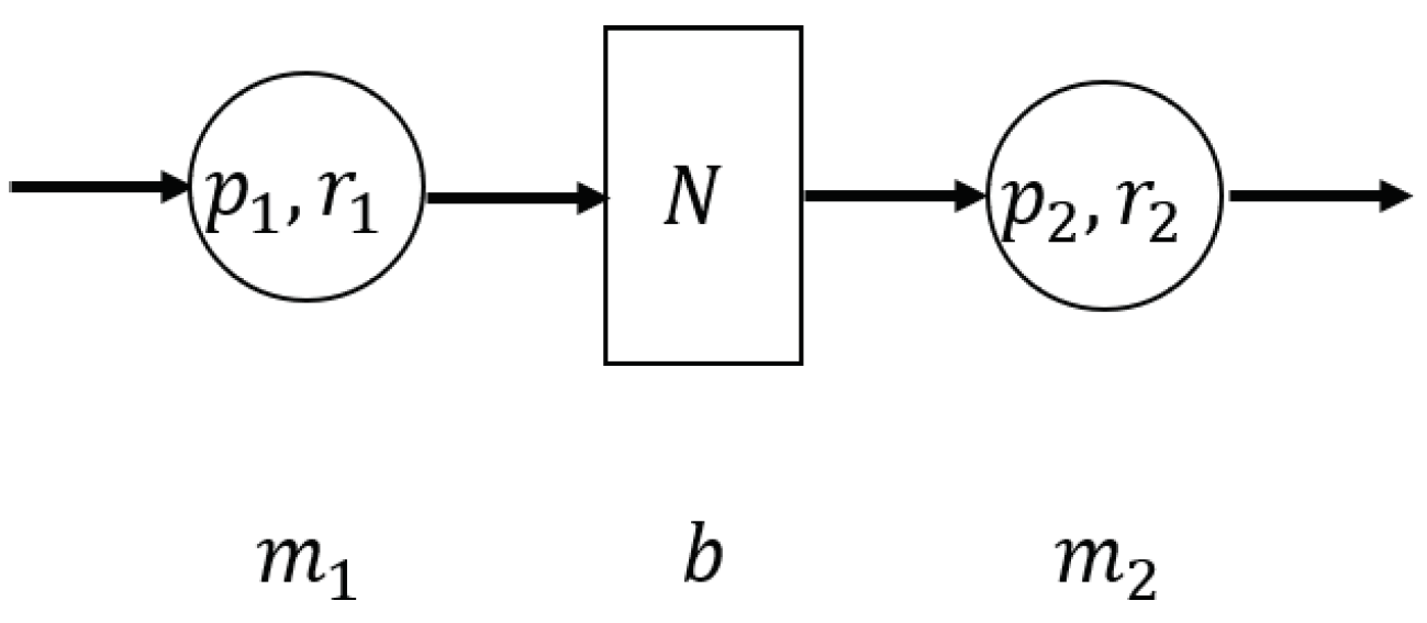
3.1. System Model

Consider a serial production line consisting of two machines and one buffer between them (see Figure 1, where the circles represent the machines, and the rectangle represents the buffer). The following assumptions are used to define the production line:

(i)

Machine $m_1$ and $m_2$ have identical cycle time $\tau$. During each time slot, where the time slot is also called the cycle time, if the machine is up, it will produce one part, otherwise, there will be no throughput. The state of the machines is determined at the beginning of each time slot.

(ii)

These two machines, $m_i$, where $i=1,2$, obey the geometric reliability model, where $p_i$ and $r_i$ are breakdown and repair probabilities, respectively. The state of a machine is denoted by $x_i\left(t\right)\in \{1=\mathrm{up},0=\mathrm{down}\}$ at time slot t. Then, the transition probabilities are as follows:

$$\begin{array}{cc}\hfill & P[x_i(t+1)=0|x_i\left(t\right)=1]=p_i\hfill \\ \hfill & P[x_i(t+1)=1|x_i\left(t\right)=1]=1-p_i\hfill \\ \hfill & P[x_i(t+1)=1|x_i\left(t\right)=1]=r_i\hfill \\ \hfill & P[x_i(t+1)=0|x_i\left(t\right)=1]=1-r_i\hfill \end{array}$$

Note that the average up- and downtime of the machines can be obtained by $t_{up}=1/p_i$ and $t_{down}=1/r_i$. Then, the machine efficiency is $e_i=\frac{t_{up}}{t_{up}+t_{down}}=\frac{r_i}{p_i+r_i}$. Both two machines are independent of each other.

(iii)

Buffer b has a finite capacity $1\le N<\infty$. The state of the buffer is determined at the end of each time slot.

(iv)

Machine $m_1$ is never starved; it will be blocked if it is up and the buffer b is full at the beginning of the time slot. Machine $m_2$ is never blocked; it will be starved if it is up and the buffer b is empty at the beginning of the time slot.

(v)

When the machine $m_i$, where $i=1,2$, is working, the energy consumption is $E_{wi}$. When the machine is idle, the energy consumption is $E_{ki}$. When the machine starts up from the down state, the energy consumption is $E_{si}$.

(vi)

The resulting productivity of the production system must meet the target, $P{R}_d$.

3.2. Problem Formulation

Based on the above model, if the machine $m_1$ or $m_2$ is up, it has three parts of energy consumption, which can be expressed as

$$\begin{array}{cc}\hfill & E_1=\underset{\mathrm{setup}}{\underbrace{\left(1-e_1\right)E_{s1}}}+\underset{\mathrm{working}}{\underbrace{E_{w1}\left(1-\left(1-e_2\right)P_N\right)}}+\underset{\mathrm{idle}}{\underbrace{E_{k1}\left(1-e_2\right)P_N}}\hfill \end{array}$$

(1)

$$\begin{array}{cc}\hfill & E_2=\underset{\mathrm{setup}}{\underbrace{\left(1-e_2\right)E_{s2}}}+\underset{\mathrm{working}}{\underbrace{E_{w2}\left(1-P_0\right)}}+\underset{\mathrm{idle}}{\underbrace{E_{k2}{P}_0}}\hfill \end{array}$$

(2)

where $P_N$ and $P_0$ stand for the probabilities of the full and empty buffer states.

There are four situations in the state of the two machines and a buffer:

• Both two machines are up with probability $e_1{e}_2$; the energy consumption is $(E_1+E_2)$;
• Machine $m_1$ is up and $m_2$ is down with probability $e_1(1-e_2)$; the energy consumption is $E_1$;
• Machine $m_1$ is down and $m_2$ is up with probability $(1-e_1)e_2$; the energy consumption is $E_2$;
• Both two machines are down with probability $(1-e_1)(1-e_2)$; no energy consumption occurs.

Therefore, summarizing the above four cases, the total energy consumption of the two-machine geometric line within a time slot can be calculated by

$$\begin{array}{c}\hfill E=e_1{e}_2(E_1+E_2)+e_1(1-e_2)E_1+(1-e_1)e_2{E}_2\end{array}$$

(3)

Then, the energy consumption minimization problem is modeled by optimizing the repair probabilities of the two machines, $(r_1,r_2)$, and the production rate is guaranteed to reach a target production rate, $P{R}_d$. The production rate $PR$ can be expressed as

$$\begin{array}{cc}\hfill PR& =e_2[1-Q(p_1,r_1,p_2,r_2,N)]=e_2(1-P_0)\hfill \end{array}$$

(4)

$$\begin{array}{cc}\hfill & \hspace{1em}\hspace{1em}\hspace{1em}\hspace{1em}=e_1[1-Q(p_2,r_2,p_1,r_1,N)]=e_1[1-(1-e_2)P_N]\hfill \end{array}$$

(5)

and is strictly increasing on $r_1$ and $r_2$ (see [35]). Thus, the energy consumption minimization problem can be mathematically formulated as

$$\begin{array}{}\mathrm{(6)}& \left(\mathrm{P}1\right)\hfill & \hfill \hspace{1em}\hspace{1em}minE=e_1{e}_2(E_1+E_2)+e_1(1-e_2)E_1+(1-e_1)e_2{E}_2\mathrm{(7)}& \hfill & \hspace{1em}\hspace{1em}\hspace{1em}\hspace{1em}s.t.e_2\left[1-Q\left(p_1,r_1,p_2,r_2,N\right)\right]⩾P{R}_d\hfill \mathrm{(8)}& \hfill & \hspace{1em}\hspace{1em}\hspace{1em}\hspace{1em}\hspace{1em}0<r_i⩽1,i=1,2\hfill \end{array}$$

where

$$\begin{array}{cc}\hfill e_i& =\frac{r_i}{p_i+r_i}\hfill \end{array}$$

(9)

$$\begin{array}{cc}\hfill Q\left(p_1,r_1,p_2,r_2,N\right)& =\left\{\begin{array}{cc}\frac{p_1{\beta }_2}{\left(p_1+r_1\right)\left(r_1+r_2-r_1{r}_2\right)},\hfill & \mathrm{if}N=1\hfill \\ \frac{p_1{\alpha }_1{\alpha }_2{\beta }_2^2\left(p_2+r_2\right)}{\Phi +\Psi +\Gamma +\Theta },\hfill & \mathrm{if}N\ne 1\hfill \end{array}\right.\hfill \end{array}$$

(10)

$$\begin{array}{cc}\hfill {\alpha }_1& =p_1+p_2-p_1{p}_2-p_2{r}_1\hfill \\ \hfill {\alpha }_2& =p_1+p_2-p_1{p}_2-p_1{r}_2\hfill \\ \hfill {\beta }_1& =r_1+r_2-r_1{r}_2-p_1{r}_2\hfill \\ \hfill {\beta }_2& =r_1+r_2-r_1{r}_2-p_2{r}_1\hfill \\ \hfill \sigma & =\frac{{\alpha }_2{\beta }_1}{{\alpha }_1{\beta }_2}\hfill \\ \hfill \Phi & =p_1{r}_2{\alpha }_1{\alpha }_2{\beta }_2\left(p_2+{\beta }_2\right)\hfill \\ \hfill \Psi & =p_1{r}_1{r}_2{\alpha }_2\left[{\beta }_2^2+p_2\left({\alpha }_1+{\beta }_1\right)\left({\alpha }_2+2{\beta }_2\right)\right]\hfill \\ \hfill \Gamma & =\sum _{k=2}^{N-1}{p}_1{p}_2{r}_1{r}_2{\left({\alpha }_2+{\beta }_2\right)}^3{\sigma }^{k-1}\hfill \\ \hfill \Theta & =p_2{r}_1{\alpha }_1{\beta }_2\left[r_2\left({\alpha }_1+{\beta }_1\right)+{\alpha }_2\left(p_1+r_1\right)\right]{\sigma }^{N-1}.\hfill \end{array}$$

(11)

Specially, ${\alpha }_1,{\alpha }_2,{\beta }_1,{\beta }_2,\sigma ,\Phi ,\Psi ,\Gamma$ and $\Theta$ are always positive.

It should be noted that $p_1$ and $p_2$ are fixed, and $r_1$ and $r_2$ are decision variables in problem (P1). According to (7), $e_i,i=1,2$ increases monotonically on $r_i$, so the upper and lower bounds of $e_i$ can be obtained. Therefore, the problem can be transformed into machine efficiency $e_1$ and $e_2$ as the decision variables:

$$\begin{gathered} \begin{array}{}\mathrm{(12)}& \left(\mathrm{P}2\right)\hfill & \hfill minE=E_{s1}\left(1-e_1\right)e_1+E_{w1}{e}_1\left(1-\left(1-e_2\right)P_N\right)+E_{k1}{e}_1\left(1-e_2\right)P_N \\ \hspace{1em}\hspace{1em}\hspace{1em}+E_{s2}\left(1-e_2\right)e_2+E_{w2}{e}_2\left(1-P_0\right)+E_{k2}{e}_2{P}_0\mathrm{(13)}& \hfill & \hspace{1em}\hspace{1em}\hspace{1em}s.t.e_2\left[1-Q(e_1,e_2,N)\right]⩾P{R}_d\hfill \mathrm{(14)}& \hfill & \hspace{1em}\hspace{1em}\hspace{1em}0<e_i⩽\frac{1}{1+p_i},i=1,2\hfill \end{array} \end{gathered}$$

Obviously, this problem transformation is equivalent. Since $p_1$ and $p_2$ are fixed, the $r_1$ and $r_2$ of the Q-function in (10) can be replaced by $e_1$ and $e_2$. It is worth mentioning that $PR$ is a function that increases monotonically with $r_i$ (or $e_i$). From [33], the maximum value of production rate is

$$\begin{array}{c}\hfill P{R}_{max}=\frac{1}{1+p_2}\left[1-Q\left(\frac{1}{1+p_1},\frac{1}{1+p_2},N\right)\right]\end{array}$$

(15)

Thus, the range of the target production rate is $0<P{R}_d\le P{R}_{max}$.

Since $PR$ is a function of $P_0$ in (4), it is also a function of $P_N$ in (5); thus, problem (P2) becomes

$$\begin{gathered} \begin{array}{}\mathrm{(16)}& \left(\mathrm{P}3\right)\hfill & \hfill minE=(E_{s1}+E_{k1})e_1-E_{s1}{e}_1^2+(E_{s2}+E_{k2})e_2-E_{s2}{e}_2^2 \\ \hspace{1em}\hspace{1em}+(E_{w1}+E_{w2}-E_{k1}-E_{k2})P{R}_d\mathrm{(17)}& & \hspace{1em}\hspace{1em}\hspace{1em}s.t.e_2\left[1-Q\left(e_1,e_2,N\right)\right]⩾P{R}_d\hfill \mathrm{(18)}& & \hspace{1em}\hspace{1em}\hspace{1em}0<e_i⩽\frac{1}{1+p_i},i=1,2\hfill \end{array} \end{gathered}$$

Similar to the analysis of the two-machine Bernoulli production line to minimize energy consumption in [34], we reconstruct the problem as below

$$\begin{gathered} \begin{array}{}\mathrm{(19)}& \left(\mathrm{P}4\right)\hfill & \hfill minE=(E_{s1}+E_{k1})e_1-E_{s1}{e}_1^2+(E_{s2}+E_{k2})e_2-E_{s2}{e}_2^2 \\ \hspace{1em}\hspace{1em}+(E_{w1}+E_{w2}-E_{k1}-E_{k2})P{R}_d\mathrm{(20)}& \hfill & \hspace{1em}\hspace{1em}\hspace{1em}s.t.e_2\left[1-Q\left(e_1,e_2,N\right)\right]=P{R}_d\hfill \mathrm{(21)}& \hfill & \hspace{1em}\hspace{1em}\hspace{1em}0<e_i⩽\frac{1}{1+p_i},i=1,2\hfill \end{array} \end{gathered}$$

Note that the (P3) and (P4) are the same except for the production rate constraint (i.e., constraint (17) and (20)), so we analyze the monotonicity of its optimal objective value with respect to $P{R}_d$. The result is shown in Theorem 1.

Theorem 1.

The optimal value, $E^{*}$, of problem (P4), is strictly increasing with respect to $P{R}_d$.

Proof. 

See Appendix A. □

Based on Theorem 1, we obtain the connection between (P3) and (P4) as follows:

Corollary 1.

Problem (P3) is exactly equivalent to problem (P4). In other words, constraint (17) in (P3) and (20) in (P4) are equivalent.

We prove this corollary by contradiction. First, assume that problems (P3) and (P4) are not equivalent, and let $P{R}^{*}$ denote the optimal production rate of (P3). Clearly, we have

$$\begin{array}{c}\hfill P{R}^{*}>P{R}_d\end{array}$$

Then we let (P4${}^{\prime })$ denote (P4) with $P{R}_d$ replaced by $P{R}^{*}$, and problem (P3) has the same optimal solution and optimal objective value as (P4${}^{\prime })$. The optimal objective values of (P4${}^{\prime })$ and (P4) are denoted by $E_1^{*}$ and $E_2^{*}$, respectively. Since $P{R}^{*}>P{R}_d$, according to Theorem 1, we have $E_1^{*}>E_2^{*}$. At the same time, the optimal solution of (P4) is also a feasible solution of (P3), i.e., $E_1^{*}⩽E_2^{*}$, which contradicts the inequality $E_1^{*}>E_2^{*}$. Therefore, the optimal production rate of (P3) is equal to $P{R}_d$.

Theorem 1 and Corollary 1 show that problems (P3) and (P4) are equivalent to each other; that is, solving (P4) is equivalent to solving (P3). In the following section, we will study the properties of (P4) and propose a solution algorithm.

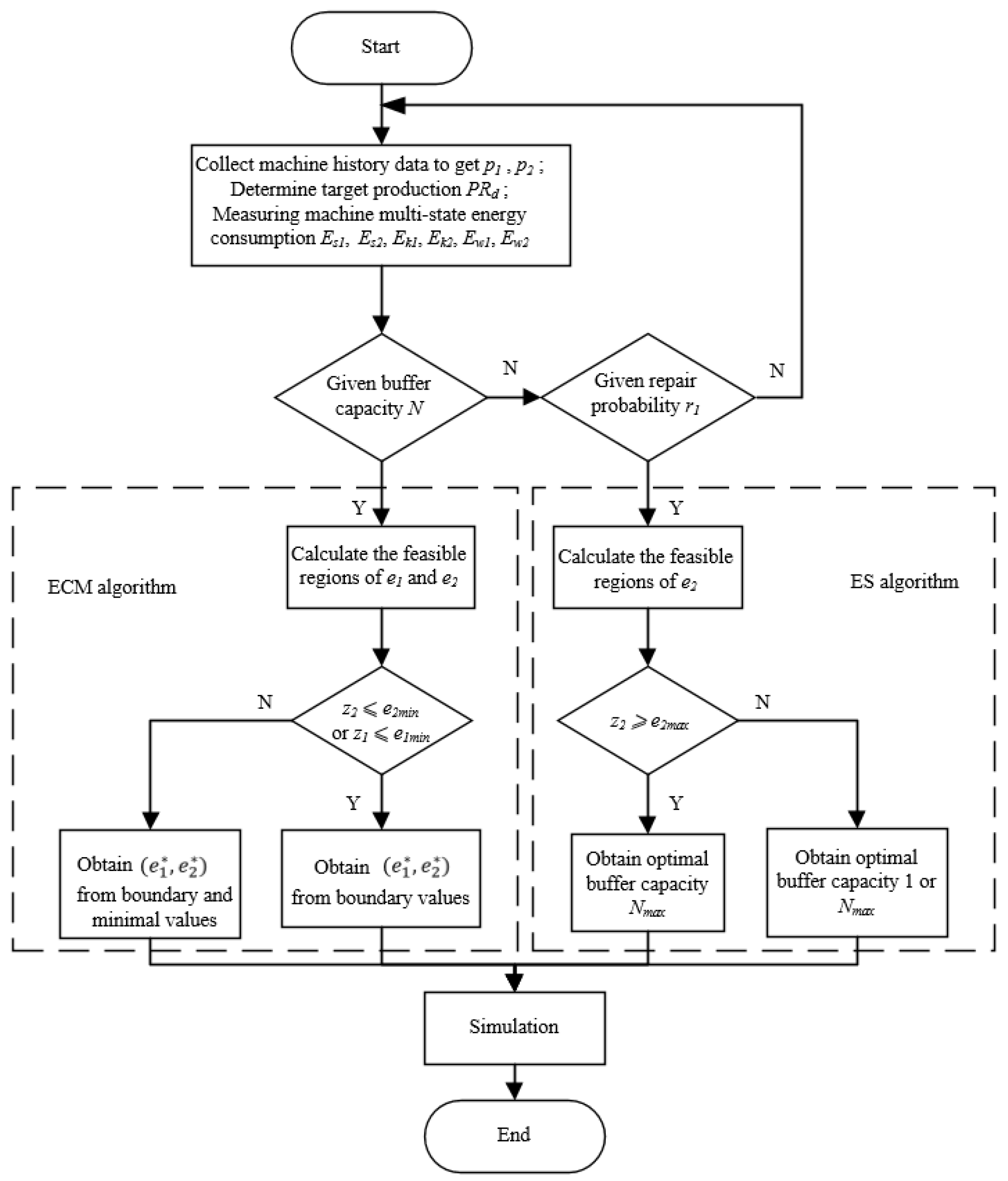
4. The ECM Algorithm

In Section 3, problems (P3) and (P4) have been shown to be equivalent. Thus, based on the analysis of the problem characteristics, an algorithm is designed for solving problem (P4) in Section 4.1. For further analysis, in Section 4.2, the problem of minimizing the energy consumption when $e_1$ is fixed with respect to the decision variables N and $e_2$ is studied.

4.1. The ECM Algorithm

In this subsection, we develop a new solution algorithm to solve the energy consumption minimum problem (P4), which is formulated in Section 3.2. Before that, we need to analyze the optimal equations of (P4), such as [33]. First, constraint (20) is one of the optimal equations, so it is necessary to explore the relationship between $e_1$ and $e_2$. The previous section noted that $PR$ is monotonically increasing with respect to $e_i$, and as shown in Figure 2, for a given $P{R}_d$, $e_2$ is a monotonically decreasing function of $e_1$.

Then, we analyze the feasible region of $e_1$ and $e_2$. Since $e_2$ is decreasing with respect to $e_1$, when $e_1$ takes the maximum value of $e_{1max},e_2$ takes the minimum value, $e_{2min}$. Similarly, when $e_2$ takes the maximum value of $e_{2max}$, the corresponding $e_1$ takes the minimum value, $e_{1min}$. Therefore, the feasible regions of $e_1$ and $e_2$ can be obtained as below:

$$\begin{array}{c}\hfill e_{imin}⩽e_i⩽\frac{1}{1+p_i},i=1,2\end{array}$$

(22)

and $e_{imin}$ can be uniquely solved by constraint (20) due to the decreasing relationship between $e_1$ and $e_2$.

Next, another optimal equation is derived below. We define an auxiliary function $h\left(e_1\right)=\frac{d{e}_2}{d{e}_1}$ as follows

$$h\left(e_1\right)=\left\{\begin{array}{cc}-\frac{p_2{e}_2^2{\left(P{R}_d-e_1{e}_2\right)}^2+p_1{p}_2{e}_1^2{e}_2^2\left(1-e_2\right)\left(e_2-P{R}_d\right)}{p_1{e}_1^2{\left(P{R}_d-e_1{e}_2\right)}^2+p_1{p}_2{e}_1^2{e}_2^2\left(1-e_1\right)\left(e_1-P{R}_d\right)},\hfill & \mathrm{if}N=1\hfill \\ -\frac{e_2^2\frac{\partial Q}{\partial e_1}}{e_2^2\frac{\partial Q}{\partial e_2}-P{R}_d},\hfill & \mathrm{if}N>1\hfill \end{array}\right.$$

(23)

where the specific form of $\frac{\partial Q}{\partial e_1}$ and $\frac{\partial Q}{\partial e_2}$ can be found in [36]. According to Numerical Facts 4.1 and 4.2 in [33], it can be known that $h\left(e_1\right)$ is continuously differentiable on $(e_{1min},e_{1max})$, and it is monotonically increasing with respect to $e_1$, with its value in $(-\infty ,0)$, which is also obtained in Figure 3.

Meanwhile, another auxiliary function $h\left(e_2\right)=\frac{d{e}_1}{d{e}_2}$ has the following formula:

$$h\left(e_2\right)=\left\{\begin{array}{cc}-\frac{p_1{e}_1^2{\left(P{R}_d-e_1{e}_2\right)}^2+p_1{p}_2{e}_1^2{e}_2^2\left(1-e_1\right)\left(e_1-P{R}_d\right)}{p_2{e}_2^2{\left(P{R}_d-e_1{e}_2\right)}^2+p_1{p}_2{e}_1^2{e}_2^2\left(1-e_2\right)\left(e_2-P{R}_d\right)},\hfill & \mathrm{if}N=1\hfill \\ -\frac{e_1^2\frac{\partial Q}{\partial e_1}}{e_1^2\frac{\partial Q}{\partial e_1}-P{R}_d},\hfill & \mathrm{if}N>1\hfill \end{array}\right.$$

(24)

It is continuously differentiable on $(e_{2min},e_{2max})$ and monotonically increasing with respect to $e_2$, with its value in $(-\infty ,0)$.

It should be noted that the energy consumption parameters and machine efficiencies directly affect the objective function in problem (P4); thus, we analyze the property of (P4) under different parameters with respect to $e_1$ and $e_2$. Since $e_2$ is an implicit function of $e_1$, i.e., $e_2\left(e_1\right)$, then $h\left(e_1\right)$ is a function of $e_1$ only. Similarly, in function $h\left(e_2\right)$, $e_1$ is an implicit function of $e_2$, which can be expressed as $e_1\left(e_2\right)$. For further analysis, the following notations are defined.

(i)

$z_1:=\frac{E_{s1}+E_{k1}}{2E_{s1}}=0.5+\frac{E_{k1}}{2E_{s1}};z_1:=\frac{E_{s2}+E_{k2}}{2E_{s2}}=0.5+\frac{E_{k2}}{2E_{s2}}$.

(ii)

$d_1:=E_{s1}+E_{k1}-2E_{s1}{e}_1;d_2:=E_{s2}+E_{k2}-2E_{s2}{e}_2.$

(iii)

$f\left(e_1\right):=-\frac{d_1}{d_2},\mathrm{when}{e}_2\ne z_2;f\left(e_2\right):=-\frac{d_2}{d_1},\mathrm{when}{e}_1\ne z_1$.

Then, the relationship between $z_1$ and $d_1$ on $e_1$ and $z_2$ and $d_2$ on $e_2$ are obtained, respectively. For example, $e_1⩽z_1$ when $d_1⩾0$, and $e_1>z_1$ when $d_1<0$. Similarly, when $d_2⩾0$, we have $e_2<z_2$, and $e_2>z_2$ when $d_2<0$. Therefore, when $z_1⩾e_{1max}$ or $z_1<e_{1min}$, $d_1⩾0$ or $d_1<0$ is always established; however, when $e_{1min}⩽z_1<e_{1max}$, there may be two cases of $d_1>0$ and $d_1⩽0$. When $z_2⩾e_{2max}$ or $z_2<e_{2min}$, we always have $d_2⩾0$ or $d_2<0$, when $e_{2min}⩽z_2<e_{2max}$; both $d_2>0$ and $d_2⩽0$ are possible.

Clearly, the optimality equation requires the partial derivative of the objective function E with respect to $e_1$, i.e.,

$$\begin{array}{c}\hfill \frac{\partial E}{\partial e_1}=E_{s1}+E_{k1}-2E_{s1}{e}_1+(E_{s2}+E_{k2}-2E_{s2}{e}_2)\frac{\mathrm{d}{e}_2}{\mathrm{d}{e}_1}\end{array}$$

(25)

Thus, the following Lemma is another optimality equation. In the following analysis, let $x\left(e_1\right)=\frac{\partial E}{\partial e_1}$ and $x\left(e_2\right)=\frac{\partial E}{\partial e_2}$.

Lemma 1.

The equality $h\left(e_i\right)=f\left(e_i\right),i=1,2$ is the sufficient and necessary condition for $x\left(e_i\right)=0$, where $e_1\ne z_1$ and $e_2\ne z_2$.

Proof. 

For $i=1$, the partial derivative of E with respect to e1 in (28) can be abbreviated as

$$\begin{array}{c}\hfill x\left(e_1\right)=d_1+d_2\times h\left(e_1\right)\end{array}$$

Since $d_2\ne 0$, we have

$$\begin{array}{c}\hfill h\left(e_1\right)=-\frac{d_1}{d_2}=f\left(e_1\right)\end{array}$$

If $i=2$, a similar result can be obtained in the same way. □

It is necessary to explore the properties of $x\left(e_1\right)$. By Lemma 1, we get that $h\left(e_1\right)=f\left(e_1\right)$ if $x\left(e_1\right)=0$. We have mentioned the properties of the $h\left(e_1\right)$ function above, then mainly analyzed the monotonicity of $f\left(e_1\right)$, that is, the properties of $d_1$ and $d_2$. For further analysis, we denote the corresponding $e_1$ value when $d_2=0$ is ${\tilde{e}}_1$. We discuss the relationship between $z_2$ and ${\tilde{e}}_1$; for instance, if ${\tilde{e}}_1<e_{1min}$, the only case that exists would be $e_2<z_2$. If ${\tilde{e}}_1⩾e_{1max}$, then only $e_2⩾z_2$ exists. However, both $e_2<z_2$ and $e_2⩾z_2$ may exist if $e_{1min}⩽{\tilde{e}}_1<e_{1max}$. The objective function E of problem (P4) can be expressed as $E\left(e_1\right)$ since $e_2$ is an implicit function of $e_1$. To sum up, the problem (P4) can be analyzed in three cases, i.e., ${\tilde{e}}_1<e_{1min},e_{1min}⩽{\tilde{e}}_1<e_{1max}$ and ${\tilde{e}}_1⩾e_{1max}$. For the first case ${\tilde{e}}_1<e_{1min}$, the properties of the problem (P4) are as follows

Observation 1.

The monotonicity and local optimum of $E\left(e_1\right)$ are listed when ${\tilde{e}}_1<e_{1min}$ and $e_1\in (e_{1min},e_{2max})$,

(i)

When $z_1⩾e_{1max}$;

• If $f\left(e_{1min}\right)>h\left(e_{1min}\right)$ and $f\left(e_{1max}\right)<h\left(e_{1max}\right)$ hold simultaneously, $E\left(e_1\right)$ has one local minimum (see Figure 4a).
• If $f\left(e_{1min}\right)<h\left(e_{1min}\right)$ and $f\left(e_{1max}\right)>h\left(e_{1max}\right)$ hold simultaneously, $E\left(e_1\right)$ has one local maximum (see Figure 4b).
• If $f\left(e_{1min}\right)<h\left(e_{1min}\right)$ and $f\left(e_{1max}\right)<h\left(e_{1max}\right)$ hold simultaneously, $E\left(e_1\right)$ is monotonically decreasing (see Figure 4c).
• If $f\left(e_{1min}\right)>h\left(e_{1min}\right)$ and $f\left(e_{1max}\right)>h\left(e_{1max}\right)$ hold simultaneously, $E\left(e_1\right)$ is monotonically increasing (see Figure 4d).

(ii)

When $e_{1min}⩽z_1<e_{1max}$, $z_1^{-}$ stands for the left limit of $z_1$;

• If $x\left(z_1^{-}\right)>0$, $E\left(p_1\right)$ has one local minimum and one local maximum, and the minimum point is to the left of the maximum (see Figure 5a).
• If $x\left(z_1^{-}\right)<0$, $E\left(p_1\right)$ is monotonically decreasing (see Figure 5b).

(iii)

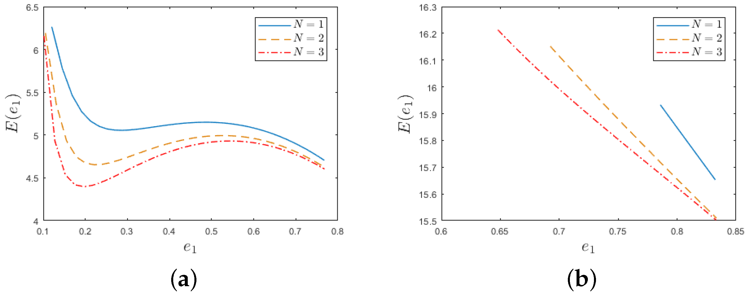
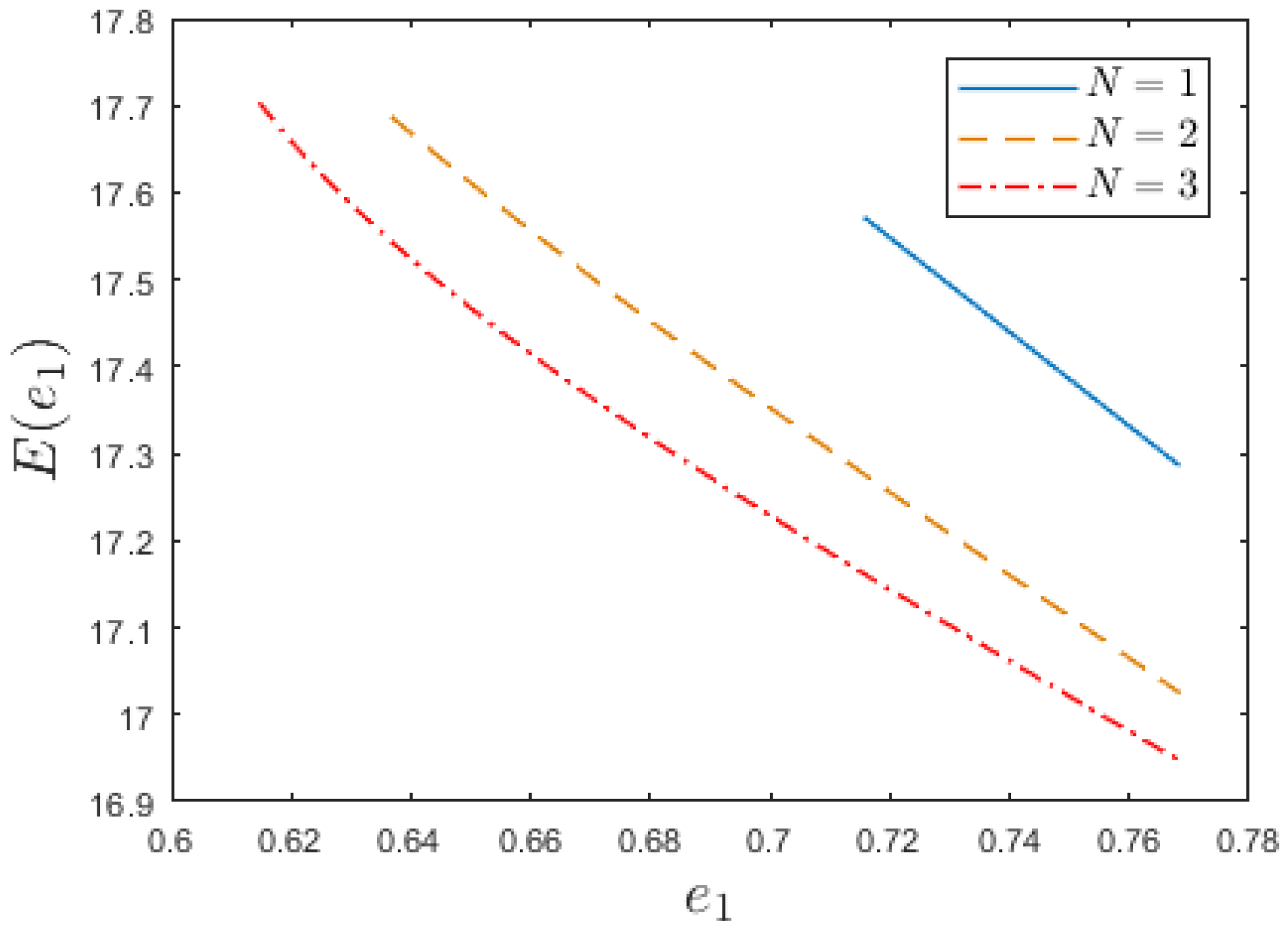
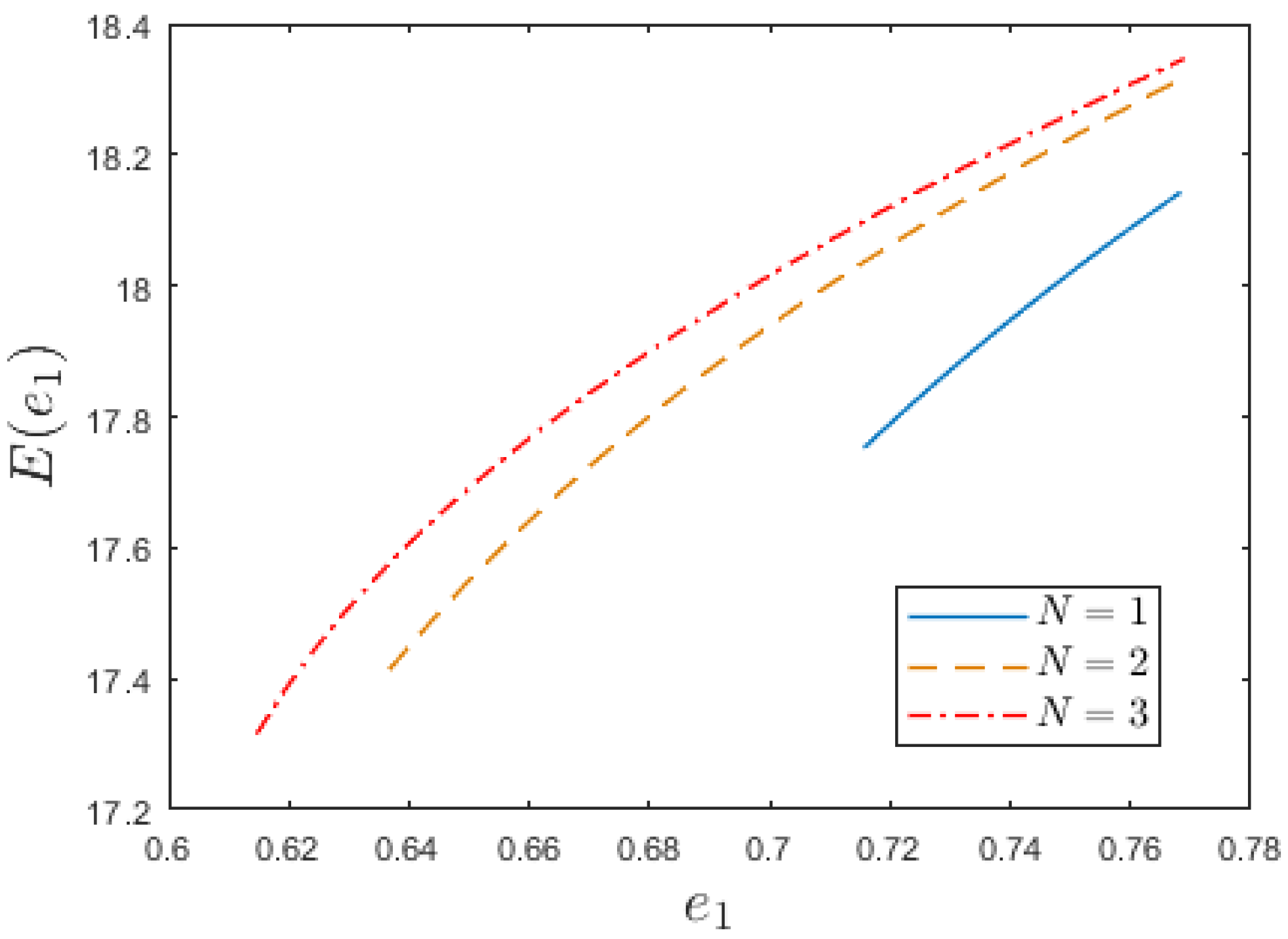
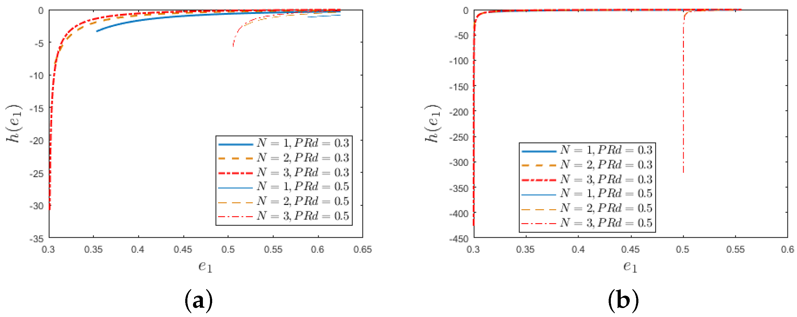
When $z_1<e_{1min}⩽e_{1max}$, $E\left(e_1\right)$ is monotonically decreasing (see Figure 6).

Figure 4. The energy consumption with respect to $e_1$ when ${\tilde{e}}_1<e_{1min},z_1⩾e_{1max}$. (a) One local minimum. (b) One local maximum. (c) Monotonically decreasing. (d) Monotonically increasing.

Figure 4. The energy consumption with respect to $e_1$ when ${\tilde{e}}_1<e_{1min},z_1⩾e_{1max}$. (a) One local minimum. (b) One local maximum. (c) Monotonically decreasing. (d) Monotonically increasing.

Figure 5. The energy consumption with respect to $e_1$ when ${\tilde{e}}_1<e_{1min},e_{1min}⩽z_1<e_{1max}$. (a) One local minimum and maximum. (b) Monotonically decreasing.

Figure 5. The energy consumption with respect to $e_1$ when ${\tilde{e}}_1<e_{1min},e_{1min}⩽z_1<e_{1max}$. (a) One local minimum and maximum. (b) Monotonically decreasing.

Figure 6. The energy consumption with respect to $e_1$ when ${\tilde{e}}_1<e_{1min},z_1<e_{1min}$.

Figure 6. The energy consumption with respect to $e_1$ when ${\tilde{e}}_1<e_{1min},z_1<e_{1min}$.

As for the case $e_{1min}⩽{\tilde{e}}_1<e_{1max}$, the properties of the problem (P4) are shown in the following observation,

Observation 2.

The monotonicity and local optimum of $E\left(e_1\right)$ are listed as follows when $e_{1min}⩽{\tilde{e}}_1<e_{1max}$ and $e_1\in (e_{1min},e_{2max})$:

(i)

when $z_1⩾e_{1max}$;

• If $\exists e^{*}\in ({\tilde{e}}_1,e_{1max})$ such that $f\left(e^{*}\right)=h\left(e^{*}\right)$, $E\left(e_1\right)$ has one local maximum and one local minimum, and the local maximum is to the left of the minimum (see Figure 7a).
• If for $\forall e_1\in [{\tilde{e}}_1,e_{1max}]$, we have $f\left(e_1\right)\ne h\left(e_1\right)$, then $E\left(e_1\right)$ is monotonically increasing (see Figure 7b).

(ii)

When $e_{1min}⩽z_1<e_{1max}$, $e^{*-}$ and $e^{*+}$ stand for the left and right limits of $e^{*}$;

• If $e^{*}\in (min({\tilde{e}}_1,z_1)$, $max({\tilde{e}}_1,z_1))$, $x\left(e^{*-}\right)<0$ and $x\left(e^{*+}\right)>0$ hold, where $f\left(e^{*}\right)=h\left(e^{*}\right)$, $E\left(e_1\right)$ has two local maximums and one local minimum, and the local minimum is in between the two maximums (see Figure 8a);
• If $e^{*}\in (min({\tilde{e}}_1,z_1)$, $max({\tilde{e}}_1,z_1))$, $x\left(e^{*-}\right)>0$ and $x\left(e^{*+}\right)<0$ hold, where $f\left(e^{*}\right)=h\left(e^{*}\right)$, $E\left(e_1\right)$ has one local maximum (see Figure 8b).

(iii)

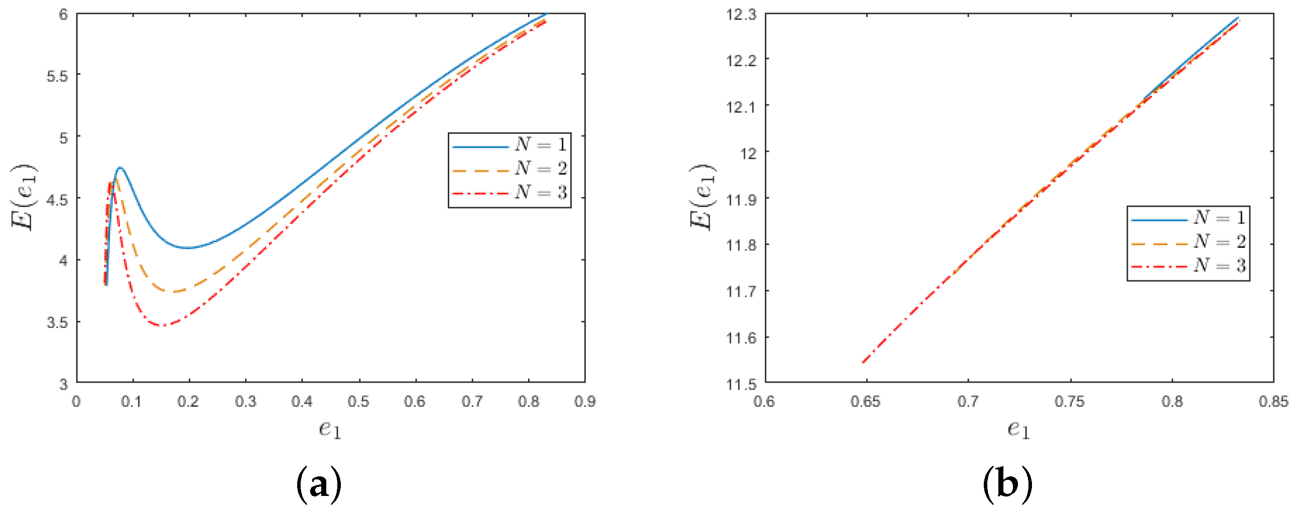
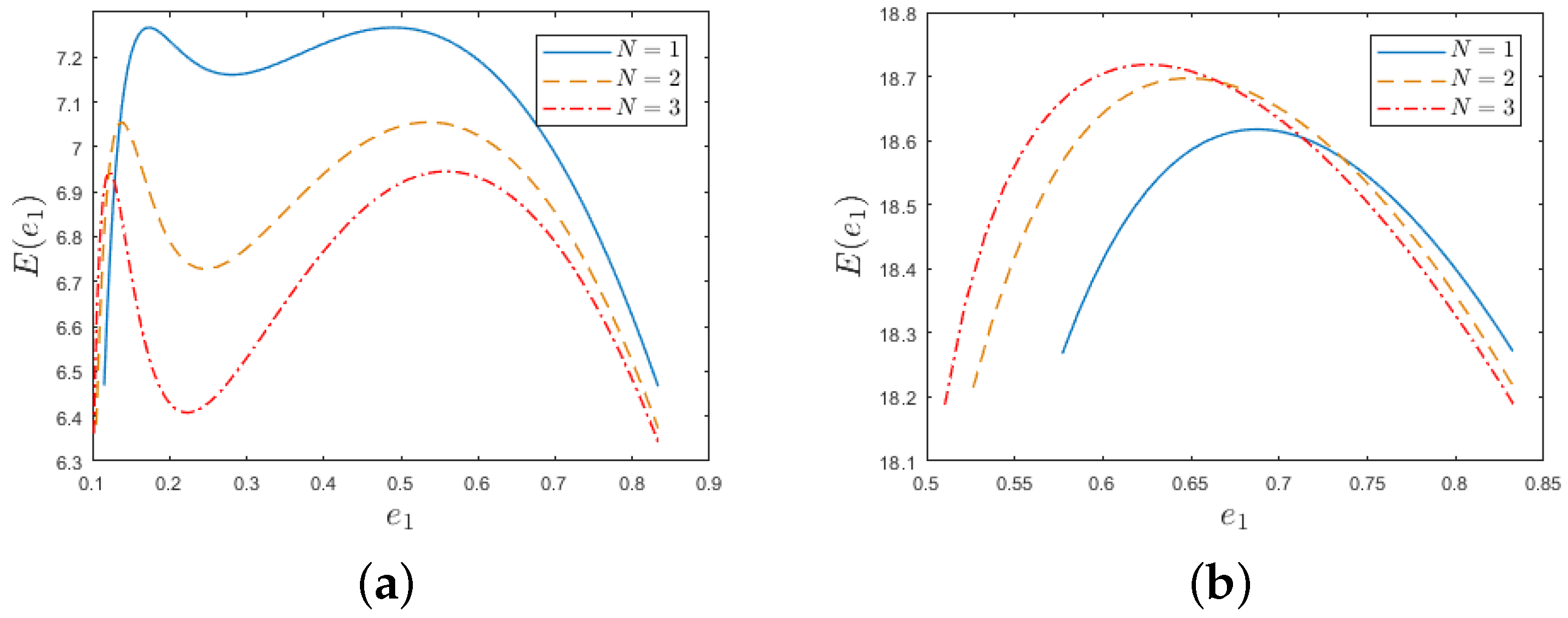
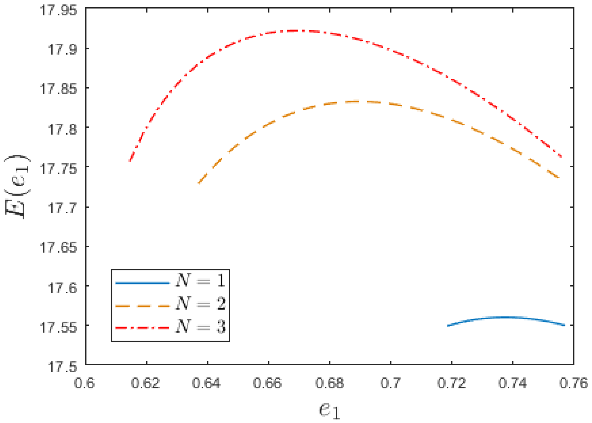
When $z_1<e_{1min}⩽e_{1max}$, $E\left(e_1\right)$ has one local maximum (see Figure 9).

Figure 7. The energy consumption with respect to $e_1$ when $e_{1min}⩽{\tilde{e}}_1<e_{1max},z_1⩾e_{1max}$. (a) One local minimum and maximum. (b) Monotonically increasing.

Figure 7. The energy consumption with respect to $e_1$ when $e_{1min}⩽{\tilde{e}}_1<e_{1max},z_1⩾e_{1max}$. (a) One local minimum and maximum. (b) Monotonically increasing.

Figure 8. The energy consumption with respect to $e_1$ when $e_{1min}⩽{\tilde{e}}_1<e_{1max},e_{1min}⩽z_1<e_{1max}$. (a) One local minimum and two local maximums. (b) One local maximum.

Figure 8. The energy consumption with respect to $e_1$ when $e_{1min}⩽{\tilde{e}}_1<e_{1max},e_{1min}⩽z_1<e_{1max}$. (a) One local minimum and two local maximums. (b) One local maximum.

Figure 9. The energy consumption with respect to $e_1$ when $e_{1min}⩽{\tilde{e}}_1<e_{1max},z_1<e_{1min}$.

Figure 9. The energy consumption with respect to $e_1$ when $e_{1min}⩽{\tilde{e}}_1<e_{1max},z_1<e_{1min}$.

For the case $e_{1min}⩽{\tilde{e}}_1<e_{1max}$, the properties of the problem (P4) are shown in Observation 3.

Observation 3.

The monotonicity and local optimum of $E\left(e_1\right)$ are listed as below when ${\tilde{e}}_1⩾e_{1max}$ and $e_1\in (e_{1min},e_{2max})$:

(i)

When $z_1⩾e_{1max}$, $E\left(e_1\right)$ is monotonically increasing (see Figure 10).

(ii)

When $e_{1min}⩽z_1<e_{1max}$;

• If $f\left(e_{1min}\right)<h\left(e_{1min}\right)$ and $f\left(e_{1max}\right)>h\left(e_{1max}\right)$ hold simultaneously, $E\left(e_1\right)$ has one local maximum (see Figure 11a).
• If $f\left(e_{1min}\right)<h\left(e_{1min}\right)$ and $f\left(e_{1max}\right)<h\left(e_{1max}\right)$ hold simultaneously, $E\left(e_1\right)$ is monotonically increasing (see Figure 11b).

(iii)

When $z_1<e_{1min}⩽e_{1max}$, $E\left(e_1\right)$ has one local maximum (see Figure 12).

Figure 10. The energy consumption with respect to $e_1$ when ${\tilde{e}}_1⩾e_{1max},z_1⩾e_{1max}$.

Figure 10. The energy consumption with respect to $e_1$ when ${\tilde{e}}_1⩾e_{1max},z_1⩾e_{1max}$.

Figure 11. The energy consumption with respect to $e_1$ when ${\tilde{e}}_1⩾e_{1max},e_{1min}⩽z_1<e_{1max}$. (a) One local maximum. (b) Monotonically increasing.

Figure 11. The energy consumption with respect to $e_1$ when ${\tilde{e}}_1⩾e_{1max},e_{1min}⩽z_1<e_{1max}$. (a) One local maximum. (b) Monotonically increasing.

Figure 12. The energy consumption with respect to $e_1$ when ${\tilde{e}}_1⩾e_{1max},z_1<e_{1min}$.

Figure 12. The energy consumption with respect to $e_1$ when ${\tilde{e}}_1⩾e_{1max},z_1<e_{1min}$.

Similarly, the energy consumption of problem (P4) is analyzed with respect to $e_2$ in the same way as with respect to $e_1$ and is not repeated here.

Based on the conclusion of the analysis of problem (P4) from the above three observations, we propose a new ECM algorithm, the pseudo-code of which is shown in Algorithm 1.

Algorithm 1: Energy consumption minimization (ECM) algorithm.

Input:$p_1,p_2,P{R}_d,N,E_{s1},E_{s2},E_{k1},E_{k2},E_{w1},E_{w2}$ 1: calculate the feasible regions of $e_1$ and $e_2$ by (20), i.e., $(e_{1min},e_{2max})$ and $(e_{1max},e_{2min}$); 2: if  $z_2⩽e_{2min}$  then 3:     find the optimal value ${\displaystyle \underset{e_1,e_2}{min}}E(e_1,e_2)$ from the candidate solution set $\Omega =\{(e_{1min},e_{2max}),(e_{1max},e_{2min})\}$. 4:     obtain the optimal system configuration $(e_1^{*},e_2^{*})$ according to (19). 5: else 6:     if $z_1⩽e_{1min}$ then 7:         find the optimal value ${\displaystyle \underset{e_1,e_2}{min}}E(e_1,e_2)$ from the candidate solution set    $\Omega =\{(e_{1min},e_{2max}),(e_{1max},e_{2min})\}$. 8:         obtain the optimal system configuration $(e_1^{*},e_2^{*})$ according to (19). 9:     else 10:         obtain the non-boundary candidate solution $({\widehat{e}}_1,{\widehat{e}}_2)$ with (20), (23), (25) 11:         find the optimal value ${\displaystyle \underset{e_1,e_2}{min}}E(e_1,e_2)$ from the candidate solution set    $\Omega =\{(e_{1min},e_{2max}),(e_{1max},e_{2min}),({\widehat{e}}_1,{\widehat{e}}_2)\}$. 12:         obtain the optimal system configuration $(e_1^{*},e_2^{*})$ according to (19). 13:     end if 14: end if Output: The optimal solution $(e_1^{*},e_2^{*})$, the candidate solution $\Omega =\{(e_{1min},e_{2max}),(e_{1max},e_{2min}),({\widehat{e}}_1,{\widehat{e}}_2)\}$ and the total energy consumption E.

4.2. The ES Algorithm

In Section 4.1, we consider the energy consumption minimization problem when $e_1$ and $e_2$ are decision variables and the buffer capacity N is a fixed value. In this subsection, we fix $e_1$ as e to solve what value of N should be taken to minimize energy consumption. In other words, problem (P4) is extended to N and $e_2$ as decision variables, i.e.,

$$\begin{gathered} \begin{array}{}\mathrm{(26)}& \left(\mathrm{P}5\right)\hfill & \hfill \hspace{1em}\hspace{1em}\hspace{1em}minE=\left(E_{s1}+E_{k1}\right)e-E_{s1}{e}^2+\left(E_{s2}+E_{k2}\right)e_2-E_{s2}{e}_2^2 \\ +\left(E_{w1}+E_{w2}-E_{k1}-E_{k2}\right)P{R}_d\mathrm{(27)}& \hfill & \hspace{1em}\hspace{1em}\hspace{1em}s.t.e_2\left[1-Q\left(e,e_2,N\right)\right]=P{R}_d,\hfill \mathrm{(28)}& \hfill & \hspace{1em}\hspace{1em}\hspace{1em}0<e_2⩽\frac{1}{1+p_2},\hfill \mathrm{(29)}& \hfill & \hspace{1em}\hspace{1em}\hspace{1em}N⩾1.\hfill \end{array} \end{gathered}$$

It is worth noting that the objective function E has only one variable, $e_2$, and constraint (27) reflects the relationship between the two variables. In order to solve this problem, we first explore the constraint (27). From the analysis of the monotonicity properties of the Q-function in [35], it can be seen that Q is strictly decreasing in N. According to (27), $e_2$ increases monotonically with Q. Thus, N is monotonically decreasing in $e_2$; see Figure 13.

Next, the derivative of the objective function E with respect to $e_2$ is

$$\begin{array}{c}\hfill \frac{\mathrm{d}E}{\mathrm{d}{e}_2}=E_{s2}+E_{k2}-2E_{s2}{e}_2\end{array}$$

(30)

Clearly, $\frac{\mathrm{d}E}{\mathrm{d}{e}_2}$ is a monotonically decreasing linear function in $e_2$, and when $e_2<\frac{E_{s2}+E_{k2}}{2E_{s}2}$, the value is greater than 0; otherwise, the value is less than 0.

Then, we find that the objective function E increases first and then decreases when $e_2=\frac{E_{s2}+E_{k2}}{2E_{s2}}$, E has a maximum value, which means when $N=1$ or $N=N_{max}$, E has a minimum value. A new algorithm is designed to solve problem (P5) with the pseudo-code shown in Algorithm 2.

Summarizing the above theoretical analysis, the framework of the present research in dealing with the energy-saving two-machine geometric serial machine line is shown in Figure 14.

Figure 13. The behavior of N with respect to $e_2$. (a) $p_1=p_2=0.6$. (b) $p_1=0.8,p_2=0.3$.

Figure 13. The behavior of N with respect to $e_2$. (a) $p_1=p_2=0.6$. (b) $p_1=0.8,p_2=0.3$.

Algorithm 2: Energy-saving (ES) algorithm.

Input:$p_1,p_2,r_1,P{R}_d,E_{s1},E_{s2},E_{k1},E_{k2},E_{w1},E_{w2}$ 1: if$z_2⩾e_{2max}$then 2:     obtain the optimal buffer capacity $N^{*}=N_{max}$. 3: else 4:     find the optimal value $\underset{N}{min}E\left(N\right)$ from the candidate solution set $\Omega =\{1,N_{max}\}$. 5:     obtain the optimal buffer capacity $N^{*}$ according to (18). 6: end if Output: The optimal solution $N^{*}$, the candidate solution $\Omega =\{1,N_{max}\}$ and the total energy consumption E.

5. Numerical and Sensitivity Analysis

In Section 4, ECM and EC algorithms are developed for solving problem (P4) and (P5), respectively. In this section, we describe numerical examples to verify these two algorithms. Specifically, the effectiveness of the algorithms is verified by a discrete production system simulation. After inputting basic parameters for a single simulation, 20,000 time slots were run, and the results output the total system energy consumption. The simulation was repeated 200 times, and the energy consumption results with 95% confidence interval were taken to verify the gap with the algorithm, thus confirming the effectiveness of the algorithm.

For problem (P4), the objective function E is determined by energy consumption parameters and machine efficiencies, which in turn are affected by buffer capacity, target production rate and fixed breakdown probabilities ($p_1,p_2$). Therefore, it is essential to evaluate the degree of the influence of these four impact factors on energy consumptions, where the energy consumption parameters are shown in

Table 1. The energy parameters of the two machines.

${\mathit{z}}_1,{\mathit{z}}_2$	Case ${}^1$	Machine 1			Machine 2
		${\mathit{E}}_{\mathit{s}\mathbf{1}}$	${\mathit{E}}_{\mathit{k}\mathbf{1}}$	${\mathit{E}}_{\mathit{w}\mathbf{1}}$	${\mathit{E}}_{\mathit{s}\mathbf{2}}$	${\mathit{E}}_{\mathit{k}\mathbf{2}}$	${\mathit{E}}_{\mathit{w}\mathbf{2}}$
$z_1>1,z_2>1$	1-1	2	4	5	3	4	9
	1-2	$2\times {10}^5$	$4\times {10}^5$	$5\times {10}^5$	3	4	9
	1-3	2	4	5	$3\times {10}^5$	$4\times {10}^5$	$9\times {10}^5$
$z_1>1,z_2<1$	2-1	3	5	8	9	2	15
	2-2	$3\times {10}^5$	$5\times {10}^5$	$8\times {10}^5$	9	2	15
	2-3	3	5	8	$9\times {10}^5$	$2\times {10}^5$	$15\times {10}^5$
$z_1<1,z_2>1$	3-1	7	1	12	4	5	10
	3-2	$7\times {10}^5$	$1\times {10}^5$	$12\times {10}^5$	4	5	10
	3-3	7	1	12	$4\times {10}^5$	$5\times {10}^5$	$10\times {10}^5$
$z_1<1,z_2<1$	4-1	9	2	14	8	3	12
	4-2	$9\times {10}^5$	$2\times {10}^5$	$14\times {10}^5$	8	3	12
	4-3	9	2	14	$8\times {10}^5$	$3\times {10}^5$	$12\times {10}^5$

${}^1$ Case: the first digit stands for the relationship between $z_i$ and 1 ($i=1,2$); the second digit represents the difference in the energy parameters of the two machines.

.

5.1. Sensitivity Analysis of Energy Consumption Parameters

In this subsection, the level of influence of the machine state energy parameters on the total energy consumption is first analyzed. Let $P{R}_d=0.3,N=1,p_1=p_2=0.5$, and the energy consumption parameters of the cases in Table 1 are used to test the proposed ECM algorithm.

The comparison results are shown in Table

Table 2. The comparison between ECM and simulation of different energy consumption parameters.

Case	ECM Algorithm					Simulation	Gap
	${\mathit{r}}_{\mathit{1}}$	${\mathit{r}}_{\mathit{2}}$	${\mathit{e}}_{\mathit{1}}$	${\mathit{e}}_{\mathit{2}}$	$\mathit{E}$
1-1	0.4463	0.4375	0.4716	0.4667	6.7982	7.0813 ($\pm 9.0099\times {10}^{-3}$)	3.9974%
1-2	0.2813	1	0.3600	0.6667	$2.2008\times {10}^5$	$2.2045\times {10}^5$ ($\pm 3.7769\times {10}^2)$	0.1681%
1-3	1	0.2813	0.6667	0.3600	$3.6312\times {10}^5$	$3.7069\times {10}^5$ ($\pm 6.4581\times {10}^2)$	2.0415%
2-1	0.2813	1	0.3600	0.6667	10.6249	10.5496 ($\pm 1.5904\times {10}^{-2})$	0.7142%
2-2	0.2813	1	0.3600	0.6667	$3.3915\times {10}^5$	$3.4420\times {10}^5(\pm 6.6497\times {10}^2)$	1.4672%
2-3	1	0.2813	0.6667	0.3600	$6.6936\times {10}^5$	$6.9244\times {10}^5(\pm 1.3302\times {10}^3)$	3.3325%
3-1	1	0.2813	0.6667	0.3600	9.7438	9.7030 ($\pm 1.4045\times {10}^{-2})$	0.4207%
3-2	0.2813	1	0.3600	0.6667	$5.2729\times {10}^5$	$5.5046\times {10}^5(\pm 1.0883\times {10}^3)$	4.2099%
3-3	1	0.2813	0.6667	0.3600	$4.2217\times {10}^5$	$4.2985\times {10}^5(\pm 7.7174\times {10}^2)$	1.7876%
4-1	1	0.2813	0.6667	0.3600	12.5565	12.4680 ($\pm 1.9177\times {10}^{-2})$	0.7105%
4-2	0.2813	1	0.3600	0.6667	$6.3937\times {10}^5$	$6.6219\times {10}^5(\pm 1.2351\times {10}^3)$	3.4456%
4-3	1	0.2813	0.6667	0.3600	$5.6233\times {10}^5$	$5.7588\times {10}^5(\pm 1.0164\times {10}^3)$	2.3537%

, and the gap between ECM and simulation is within 5%, which proves the correctness of ECM algorithm. At the same time, we find that when the energy consumption parameters of the two machines differ significantly, the total energy consumption is determined by the machine with the larger parameter, and its machine efficiency is taken to the minimum value.

5.2. Sensitivity Analysis of Buffer Capacity

In this subsection, the impact of buffer capacity on total energy consumption is considered, so N was set to 1, 2, and 3, respectively. The other impact factors were guaranteed to be constant so that $P{R}_d=0.3$, $p_1=p_2=0.5$, and cases 1-1, 2-1, 3-1, and 4-1 were selected for the numerical analysis.

The comparison results of the ECM algorithm and simulation based on different buffer capacities are listed in

Table A1. The comparison between ECM and simulation of different N.

N	Case	ECM Algorithm					Simulation	Gap
		${\mathit{r}}_{\mathbf{1}}$	${\mathit{r}}_{\mathbf{2}}$	${\mathit{e}}_{\mathbf{1}}$	${\mathit{e}}_{\mathbf{2}}$	$\mathit{E}$
1	1-1	0.4463	0.4375	0.4716	0.4667	6.7982	7.0813 $(\pm 9.0099\times {10}^{-3}$)	3.9974%
	2-1	0.2813	1	0.3600	0.6667	10.6249	10.5496 $(\pm 1.5904\times {10}^{-2})$	0.7142%
	3-1	1	0.2813	0.6667	0.3600	9.7438	9.7030 $(\pm 1.4045\times {10}^{-2})$	0.4207%
	4-1	1	0.2813	0.6667	0.3600	12.5565	12.4680 $(\pm 1.9177\times {10}^{-2})$	0.7105%
2	1-1	0.3559	0.3434	0.4158	0.4072	6.3019	6.4776 $(\pm 8.9388\times {10}^{-3})$	2.7125%
	2-1	0.2249	1	0.3103	0.6667	10.3266	9.8413 $(\pm 1.4998\times {10}^{-2})$	4.9316%
	3-1	1	0.2249	0.6667	0.3103	9.4294	9.0171 $(\pm 1.6083\times {10}^{-2})$	4.5729%
	4-1	1	0.2249	0.6667	0.3103	12.2760	11.7154 $(\pm 2.0028\times {10}^{-2})$	4.7848%
3	1-1	0.3175	0.3083	0.3884	0.3814	6.0620	6.0774 $(\pm 8.1676\times {10}^{-3})$	0.2526%
	2-1	0.2165	1	0.3022	0.6667	10.2767	9.7356 $(\pm 1.4804\times {10}^{-2})$	5.5581%
	3-1	1	0.2165	0.6667	0.3022	9.3765	8.9209 $(\pm 1.5936\times {10}^{-2})$	5.1077%
	4-1	1	0.2165	0.6667	0.3022	12.2267	11.5895 $(\pm 1.9345\times {10}^{-2})$	5.4984%

. It can be observed that the gap between the ECM algorithm and the simulation does not exceed 5.6%, which justifies the reliability of EMS algorithm. It is worth noting that the total energy consumption shows a decreasing trend when the buffer capacity becomes larger, keeping other parameters constant.

5.3. Sensitivity Analysis of $P{R}_d$

In this subsection, we design numerical examples to analyze the impact of expected production rate with respect to energy consumption. Let $N=1,p_1=p_2=0.5$. We chose different values of $P{R}_d$ as 0.05, 0.3 and 0.55 and selected cases 1-1, 2-1, 3-1 and 4-1 for the sensitivity analysis.

With the buffer capacity and breakdown probabilities given, the total energy consumption E and gap for different production rate $P{R}_d$ are displayed in

Table A2. The comparison between ECM and simulations of different $P{R}_d$.

${\mathit{PR}}_{\mathit{d}}$	Case	ECM Algorithm					Simulation	Gap
		${\mathit{r}}_{\mathbf{1}}$	${\mathit{r}}_{\mathbf{2}}$	${\mathit{e}}_{\mathbf{1}}$	${\mathit{e}}_{\mathbf{2}}$	$\mathit{E}$
0.05	1-1	0.0840	0.0764	0.1438	0.1325	1.9963	1.9659 $(\pm 6.0288\times {10}^{-3})$	1.5439%
	2-1	0.0850	0.0755	0.1453	0.1312	3.1876	3.1425 $(\pm 9.7438\times {10}^{-3})$	1.4361%
	3-1	0.0890	0.0725	0.1511	0.1267	2.9249	2.9003 $(\pm 7.7031\times {10}^{-3})$	0.8492%
	4-1	0.0810	0.0790	0.1394	0.1365	3.7612	3.6787 $(\pm 9.8294\times {10}^{-3})$	2.2440%
0.3	1-1	0.4463	0.4375	0.4716	0.4667	6.7982	7.0813 $(\pm 9.0099\times {10}^{-3})$	3.9974%
	2-1	0.2813	1	0.3600	0.6667	10.6249	10.5496 $(\pm 1.5904\times {10}^{-2})$	0.7142%
	3-1	1	0.2813	0.6667	0.3600	9.7438	9.7030 $(\pm 1.4045\times {10}^{-2})$	0.4207%
	4-1	1	0.2813	0.6667	0.3600	12.5565	12.4680 $(\pm 1.9177\times {10}^{-2})$	0.7105%
0.55	1-1	0.9706	1	0.6600	0.6667	9.7221	9.5312 $(\pm 8.8904\times {10}^{-3})$	2.0029%
	2-1	0.9706	1	0.6600	0.6667	16.1065	15.6774 $(\pm 1.7179\times {10}^{-2})$	2.7373%
	3-1	1	0.9706	0.6667	0.6600	15.2203	14.8304 $(\pm 1.5953\times {10}^{-2})$	2.6287%
	4-1	1	0.9706	0.6667	0.6600	18.6585	18.0036 $(\pm 1.8124\times {10}^{-2})$	3.6376%

. The gap between the ECM algorithm and the simulation does not exceed 4 %, which verifies the accuracy of the algorithm. Table A2 shows that the energy consumption is monotonically increasing with respect to $P{R}_d$, and it is also noticable that the energy consumption is minimized when the machine efficiencies take boundaries for larger $P{R}_d$.

5.4. Sensitivity Analysis of $p_1,p_2$

In this subsection, numerical examples are designed to analyze the impact of breakdown probabilities on total energy consumption, ensuring that other parameters are constant, e.g., $N=1$ and $P{R}_d=0.3$. Three different sets of breakdown probabilities (0.2, 0.1), (0.5, 0.5) and (0.8, 0.9) were chosen, and cases 1-1, 2-1, 3-1 and 4-1 were selected as energy consumption parameter inputs.

The results of the ECM algorithm and simulation comparison based on different breakdown probabilities are listed in

Table A3. The comparison between ECM and simulations of different $p_1,p_2$.

${\mathit{p}}_1$	${\mathit{p}}_2$	Case	ECM Algorithm					Simulation	Gap
			${\mathit{r}}_{\mathbf{1}}$	${\mathit{r}}_{\mathbf{2}}$	${\mathit{e}}_{\mathbf{1}}$	${\mathit{e}}_{\mathbf{2}}$	$\mathit{E}$
0.2	0.1	1-1	0.1944	0.1304	0.4911	0.5660	7.2895	7.0010 $(\pm 1.2008\times {10}^{-2})$	4.1211%
		2-1	0.0957	1	0.3236	0.9087	9.6389	9.4890 $(\pm 2.2928\times {10}^{-2})$	1.5797%
		3-1	1	0.0545	0.8333	0.3528	9.2826	8.9229 $(\pm 2.8355\times {10}^{-2})$	4.0315%
		4-1	1	0.0545	0.8333	0.3528	12.1015	11.6417 $(\pm 3.4061\times {10}^{-2})$	3.9495%
0.5	0.5	1-1	0.4463	0.4375	0.4716	0.4667	6.7982	7.0813 $(\pm 9.0099\times {10}^{-3})$	3.9974%
		2-1	0.2813	1	0.3600	0.6667	10.6249	10.5496 $(\pm 1.5904\times {10}^{-2})$	0.7142%
		3-1	1	0.2813	0.6667	0.3600	9.7438	9.7030 $(\pm 1.4045\times {10}^{-2})$	0.4207%
		4-1	1	0.2813	0.6667	0.3600	12.5565	12.4680 $(\pm 1.9177\times {10}^{-2})$	0.7105%
0.8	0.9	1-1	0.5595	0.5646	0.4116	0.3855	6.1833	6.0434 $(\pm 8.8105\times {10}^{-3})$	2.3155%
		2-1	0.3965	1	0.3314	0.5263	10.4181	10.2493 $(\pm 8.3501\times {10}^{-3})$	1.6471%
		3-1	1	0.4119	0.5554	0.3140	9.5154	9.2318 $(\pm 8.6999\times {10}^{-3})$	3.0717%
		4-1	1	0.4119	0.5554	0.3140	12.2984	11.9102 $(\pm 1.1362\times {10}^{-2})$	2.4197%

. It can be discovered that the breakdown probabilities do not have a significant effect on the total energy consumption. Meanwhile, the ECM algorithm is valid since the difference between algorithm and simulation is less than 4.2%.

5.5. ES Algorithm and Simulation Comparison

In this subsection, we design numerical examples and verify the effectiveness of the EC algorithm by simulation. Specifically, we set $p_1=0.8,p_2=0.1$, $N\in [1,20]$ and choose cases 1-1, 2-1, 3-1, and 4-1 for the analysis.

The comparison results of the ES algorithm and simulation are shown in

Table 3. The comparison between the ES algorithm and simulation ($p_1=0.8,p_2=0.1$).

${\mathit{PR}}_{\mathit{d}}$	${\mathit{r}}_1$	Case	ES Algorithm				Simulation	Gap
			${\mathit{r}}_{\mathbf{2}}$	${\mathit{e}}_{\mathbf{2}}$	$\mathit{N}$	$\mathit{E}$
0.3	0.4	1-1	0.0732	0.4226	20	6.0002	5.6751 ($\pm 2.0309\times {10}^{-2})$	5.7281%
		2-1	0.4000	0.8000	1	10.1733	10.1246 $(\pm 1.1636\times {10}^{-2})$	0.4810%
		3-1	0.0732	0.4226	20	9.7779	9.5336 $(\pm 1.2145\times {10}^{-2})$	2.5629%
		4-1	0.0732	0.4226	20	12.1865	12.9396 $(\pm 1.7163\times {10}^{-2})$	5.8204%
0.4	0.6	1-1	0.1123	0.5290	20	7.4676	7.0791 $(\pm 6.9913\times {10}^{-3})$	5.4878%
		2-1	0.5719	0.8512	1	12.1200	12.0232 $(\pm 1.3397\times {10}^{-2})$	0.8047%
		3-1	0.1123	0.5290	20	12.1846	11.7161 $(\pm 1.2876\times {10}^{-2})$	3.9991%
		4-1	0.5719	0.8512	1	15.0282	14.7474 $(\pm 1.5572\times {10}^{-2})$	1.9039%
0.5	0.9	1-1	0.1267	0.5588	20	8.5907	8.7511 $(\pm 4.6700\times {10}^{-3})$	1.8332%
		2-1	0.6835	0.8724	1	14.1413	12.7798 $(\pm 1.4799\times {10}^{-2})$	4.3490%
		3-1	0.1267	0.5588	20	14.0535	14.4791 $(\pm 7.6329\times {10}^{-3})$	2.9396%
		4-1	0.6835	0.8724	1	17.3089	17.4639 $(\pm 9.3382\times {10}^{-3})$	0.8875%

. For cases 1-1 and 3-1, the minimum energy consumption corresponds to N always being 20 due to the fact that $z_2$ is constantly greater than 1 for both cases. As the gap between the ES algorithm and simulation is within 5.83%, the algorithm is valid.

5.6. Discussion and Imitations

There are various approaches to reduce energy consumption in production systems, such as meta-heuristic algorithms, heuristic algorithms for stochastic optimization problems, and machine learning. In the metaheuristic algorithm, for instance, Gao et al. [24] use the artificial bee colony algorithm to solve the deterministic scheduling problem and can only obtain the non-exact solutions. Conversely, in the proposed algorithms, the exact solutions can be attained. In addition, it is observed that ECM and ES algorithms also have good performance in terms of the speed of solving. Yan and Liu [33] and Pei et al. [34] deal with stochastic system optimization problems and propose a heuristic algorithm solution model based on problem characteristics. However, the objective function of [33] contains only the normal working energy consumption, and the productivity constraint of [34] is for Bernoulli reliability machines. In contrast, the present model is a geometric production line with multi-state energy consumption rates. Additionally, the most distinct feature of the present paper is that the buffer capacity is regarded as a decision variable. Machine learning is also a great tool to help analyze the production systems with industrial big data. Li et al. [22] apply the Q-learning algorithm to search for the optimal control policy to reduce energy consumption. However, its lack of explainable results limits its usage in several specific scenarios, where the methods with solid theoretical knowledge are more favored. Fortunately, with the help of production system engineering, we obtain the system dynamics of the geometric machine line by constructing a mathematical model of the problem. Then, the essential properties of the production system are analyzed by exploiting the unique features of the system. To sum up, the deterministic problem can be searched and solved using the meta-heuristic algorithm. When the production systems are volatile, the heuristic algorithm can be designed to solve the problem exactly based on the problem characteristics. If the production system has large data, the machine learning method can be preferred.

Nevertheless, since the actual production line is too complex for us to analyze directly, it is usually simplified for research purposes. In order to obtain closed-form results, one way to simplify the actual production line is by making assumptions, even though these assumptions could render the research limited. One of the many possible future research directions would be to relax the one product at a cycle time assumption. In fact, the machines could be capable of producing multiple units per unit of cycle time, which means that they are batch servers; the energy-saving strategies of such a production line would be challenging to explore. Additionally, it is assumed in the present paper that the two machines have identical cycle times, i.e., they are working synchronously. However, the cycle times of real machines are often vastly different, and how to handle such an asynchronous production line will be an exciting extension of the present study. Furthermore, the two machines obey the geometric reliability model, which is one type of discrete event system, and we believe that the continuous time-based approaches, despite their complexity, are more suitable to the actual factory floor situation and thereby are worthy of investigation. Another potential improvement lies in the discrete simulation sector. Currently, the simulation can only deliver results with the data obtained from the algorithms, and each simulation run takes a long period of time. Additionally, the simulation parameters are randomly generated without incorporating the actual production site data. In the future, simulation and optimization models can be combined to improve the algorithm efficiency. The derived optimal solution will be verified via a simulation with parameters built upon actual field data.

6. Conclusions

In this paper, a nonlinear model to reflect the energy consumption in a two-machine serial production line with geometric reliability and a finite buffer is introduced. The goal is to minimize the total energy consumption while ensuring the target productivity. By exploring the problem properties, a heuristic algorithm based on the monotonicity and the local optimum, i.e., the ECM algorithm, is proposed. Specifically, the energy-saving manufacturing system model is discussed under three problem settings. We also investigate the problem of minimizing energy consumption when the buffer capacity is regarded as a decision variable, and a separate ES algorithm is designed for solving it. In order to verify the validity of the ECM and ES algorithms, numerical examples are included to compare the analytical results with simulations. The influences of energy consumption parameters, such as buffer capacity, target productivity, and breakdown probabilities, on the overall system energy consumption are also investigated.

In the future, the approaches and results of the present paper can be extended to more complex production lines, such as longer serial lines and assembly lines, and machines with other reliability features may also be of interest, such as the exponential and non-Markovian (i.e., Weibull, gamma, log-normal, etc.) machines. Second, the results could be applied to actual plants to design and control production lines for reducing energy consumption. Third, more states of the system could be considered in the actual operation of the manufacturing system, for instance, the warm-up, the cool-down, the sleep mode, and the energy consumption of the buffer. Finally, the machine can produce more than one part during each cycle time.

References

- Kolta, T. Selecting Equipment to Control Air Pollution from Automotive Painting Operations. In Technical Report; SAE Technical Paper; Auto. Eng.: Warrendale, PA, USA, 1992. [Google Scholar]
- Galitsky, C.; Worrell, E. Energy Efficiency Improvement and Cost Saving Opportunities for the Vehicle Assembly Industry: An Energy Star Guide for Energy and Plant Managers. In Technical Report; Lawrence Berkeley National Lab. (LBNL): Berkeley, CA, USA, 2008. [Google Scholar]
- Altiok, T. Performance Analysis of Manufacturing Systems; Springer: Belin, Germany, 1997. [Google Scholar]
- Askin, R.G.; Standridge, C.R. Modeling and Analysis of Manufacturing Systems; Wiley: New York, NY, USA, 1993. [Google Scholar]
- Li, J.; Meerkov, S.M. Production Systems Engineering; Springer: New York, NY, USA, 2009. [Google Scholar]
- Pei, Z.; Lu, H.; Jin, Q.; Zhang, L. Target-based distributionally robust optimization for single machine scheduling. Eur. J. Oper. Res. 2022, 299, 420–431. [Google Scholar] [CrossRef]
- Kim, W.S.; Morrison, J.R. The throughput rate of serial production lines with deterministic process times and random setups: Markovian models and applications to semiconductor manufacturing. Comput. Oper. Res. 2015, 53, 288–300. [Google Scholar] [CrossRef]
- Pei, Z.; Wan, M.; Jiang, Z.Z.; Wang, Z.; Dai, X. An approximation algorithm for unrelated parallel machine scheduling under tou electricity tariffs. IEEE Trans. Autom. Sci. Eng. 2020, 18, 743–756. [Google Scholar] [CrossRef]
- Tu, J.; Zhang, L. Performance analysis and optimisation of Bernoulli serial production lines with dynamic real-time bottleneck identification and mitigation. Int. J. Prod. Res. 2022, 60, 3989–4005. [Google Scholar] [CrossRef]
- Arinez, J.; Biller, S.; Meerkov, S.M.; Zhang, L. Quality/quantity improvement in an automotive paint shop: A case study. IEEE Trans. Autom. Sci. Eng. 2009, 7, 755–761. [Google Scholar] [CrossRef]
- Hillier, M. Designing unpaced production lines to optimize throughput and work-in-process inventory. IIE Trans. 2013, 45, 516–527. [Google Scholar] [CrossRef]
- Biller, S.; Meerkov, S.M.; Yan, C.B. Raw material release rates to ensure desired production lead time in Bernoulli serial lines. Int. J. Prod. Res. 2013, 51, 4349–4364. [Google Scholar] [CrossRef]
- Shen, X.; Li, N. Scheduling policies analysis for matching operations in bernoulli selective assembly lines. Int. J. Prod. Res. 2022, 60, 3965–3988. [Google Scholar] [CrossRef]
- Menghi, R.; Papetti, A.; Germani, M.; Marconi, M. nergy efficiency of manufacturing systems: A review of energy assessment methods and tools. J. Clean. Prod. 2019, 240, 118276. [Google Scholar] [CrossRef]
- Zhang, Y.; Yang, J.; Liu, M. Enterprises’ energy-saving capability: Empirical study from a dynamic capability perspective. Renew. Sustain. Energy Rev. 2022, 162, 112450. [Google Scholar]
- Li, L.; Sun, Z. Dynamic Energy Control for Energy Efficiency Improvement of Sustainable Manufacturing Systems Using Markov Decision Process. IEEE Trans. Syst. Man Cybern. Syst. 2013, 43, 1195–1205. [Google Scholar] [CrossRef]
- Mashaei, M.; Lennartson, B. Energy Reduction in a Pallet-Constrained Flow Shop Through On–Off Control of Idle Machines. IEEE Trans. Autom. Sci. Eng. 2013, 1, 45–56. [Google Scholar] [CrossRef]
- Cui, P.H.; Wang, J.Q.; Li, Y.; Yan, F.Y. Energy-efficient control in serial production lines: Modeling, analysis and improvement. J. Manuf. Syst. 2021, 60, 11–21. [Google Scholar] [CrossRef]
- Frigerio, N.; Matta, A. Analysis on Energy Efficient Switching of Machine Tool With Stochastic Arrivals and buffer information. IEEE Trans. Autom. Sci. Eng. 2016, 1, 238–246. [Google Scholar] [CrossRef]
- Renna, P.; Materi, S. Switch off policies in job-shop manufacturing systems including workload evaluation. Int. J. Manag. Sci. Eng. Manag. 2021, 16, 254–263. [Google Scholar] [CrossRef]
- Jia, Z.; Zhang, L.; Arinez, J.; Xiao, G. Performance analysis for serial production lines with Bernoulli machines and real-time WIP-based machine switch-on/off control. Int. J. Prod. Res. 2016, 54, 6285–6301. [Google Scholar] [CrossRef]
- Li, Y.; Cui, P.H.; Wang, J.Q.; Chang, Q. Energy-saving control in multistage production systems using a state-based method. IEEE Trans. Autom. Sci. Eng. 2021. [Google Scholar] [CrossRef]
- Chen, G.; Zhang, L.; Arinez, J.; Biller, S. Energy-efficient production systems through schedule-based operations. IEEE Trans. Autom. Sci. Eng. 2013, 1, 27–37. [Google Scholar] [CrossRef]
- Gao, Y.; Wang, Q.; Feng, Y.; Zheng, H.; Zheng, B.; Tan, J. An energy-saving optimization method of dynamic scheduling for disassembly line. Energies 2018, 11, 1261. [Google Scholar] [CrossRef]
- Li, S.; Liu, F.; Zhou, X. Multi-objective energy-saving scheduling for a permutation flow line. Proc. Inst. Mech. Eng. Part J. Eng. Manuf. 2018, 232, 879–888. [Google Scholar] [CrossRef]
- Su, W.; Xie, X.; Li, J.; Zheng, L. Improving energy efficiency in Bernoulli serial lines: An integrated model. Int. J. Prod. Res. 2016, 54, 3414–3428. [Google Scholar] [CrossRef]
- Yan, C.B.; Cheng, X.; Gao, F.; Guan, X. Formulation and Solution Methodology for Reducing Energy Consumption in Two-Machine Bernoulli Serial Lines. IEEE Trans. Autom. Sci. Eng. 2022, 19, 522–530. [Google Scholar] [CrossRef]
- Yan, C.B. Analysis and Optimization of Energy Consumption in Two-Machine Bernoulli Lines with General Bounds on Machine Efficiency. IEEE Trans. Autom. Sci. Eng. 2021, 18, 151–163. [Google Scholar] [CrossRef]
- Su, W.; Xie, X.; Li, J.; Zheng, L.; Feng, S.C. Reducing energy consumption in serial production lines with Bernoulli reliability machines. Int. J. Prod. Res. 2017, 55, 7356–7379. [Google Scholar] [CrossRef]
- Yan, C.B.; Zheng, Z. Problem Formulation and Solution Methodology for Energy Consumption Optimization in Bernoulli Serial Lines. IEEE Trans. Autom. Sci. Eng. 2021, 18, 776–790. [Google Scholar] [CrossRef]
- Yan, C.B.; Zheng, Z. An effective and efficient divide-and-conquer algorithm for energy consumption optimisation problem in long Bernoulli serial lines. Int. J. Prod. Res. 2021, 59, 7018–7036. [Google Scholar] [CrossRef]
- Cheng, X.; Yan, C.B.; Gao, F. Energy cost optimisation in two-machine Bernoulli serial lines under time-of-use pricing. Int. J. Prod. Res. 2022, 60, 3948–3964. [Google Scholar] [CrossRef]
- Yan, C.B.; Liu, L. Energy Consumption Optimization in Two-Machine Geometric Serial Lines. In Proceedings of the 2020 IEEE 16th International Conference on Automation Science and Engineering (CASE), Hong Kong, China, 20–21 August 2020; pp. 830–835. [Google Scholar]
- Pei, Z.; Yang, P.; Wang, Y.; Yan, C.B. Energy consumption control in the two-machine Bernoulli serial production line with setup and idleness. Int. J. Prod. Res. 2022, 1–20. [Google Scholar] [CrossRef]
- Li, J. Production Variability in Manufacturing Systems: A Systems Approach; University of Michigan: Ann Arbor, MI, USA, 2000. [Google Scholar]
- Yan, C.B.; Liu, L.; Derivatives of Key Functions w.r.t. Machine Efficiencies in Two-Machine Geometric Line. 2020. Available online: http://gr.xjtu.edu.cn/web/chaoboyan/reports (accessed on 1 April 2020).