The Heterogeneous Effect of Economic Complexity and Export Quality on the Ecological Footprint: A Two-Step Club Convergence and Panel Quantile Regression Approach

Abstract

This research aims to answer two fundamental questions of the present time: First, what is the impact of the increasing complexity of economic structures and the production of complex goods on the environment? Second, can increasing export quality lead to the improvement of the environment? Given that the relationship of the ecological footprint and its determinants has been revealed to be nonlinear, the use of the quantile approach is supported. This finding led us to the central hypothesis of this research: economic complexity and export quality first deteriorate the ecological footprint (i.e., in lower quantiles), and the middle and higher quantiles contribute to reducing or mitigating environmental damage. The effect of economic complexity and export quality on the ecological footprint was researched using a two-step approach. First, club convergence was applied to identify the countries that follow a similar convergence path. After this, panel quantile regression was used to determine the explanatory power of economic complexity and export quality on the ecological footprint of 98 countries from 1990 to 2014. The club convergence revealed four convergent groups. Panel quantile regression was used because the relationship between the ecological footprint and its explanatory variables was shown to be nonlinear for the group of countries identified by the club convergence approach. GDP, nonrenewable energy consumption, and the population damage the environment. Urbanisation contributes to reducing the ecological footprint. Export quality and trade openness reduce the ecological footprint, but not at all quantiles. The effect of trade openness mitigating the ecological footprint is lost at the 90th quantile. Export quality becomes a reducer of the ecological footprint in the 50th quantile or above, and in the higher quantiles, its contribution to reducing the footprint is vast. Economic complexity aggravates the ecological footprint in low quantiles (10th), becomes non-statistically significant in the 25th quantile, and reduces the ecological footprint in higher quantiles. Policymakers must identify the impact of the ecological footprint and consider the demand and supply side of economics.

1. Introduction

The motivation for this research was to assess if the generally desired evolution of economies toward more complex ones and the improvement of their exports are helping to mitigate the degradation of the environment (here measured as the ecological footprint). Indeed, the most pertinent issue facing societies today is the compatibility of economic growth with the maintenance of environmental quality. Environmental degradation caused by human activities due to rapid economic growth, increasing energy demand, industrialisation, and trade expansion has become a global issue. Hence, policymakers and governments have sought solutions to this problem. For this purpose, countries have held conferences and made agreements to take measures to combat environmental degradation (e.g., the Paris Climate Change Conference 2015; the United Nations). The novelty of this research is verifying how countries with similar ecological footprint pathways respond to economic variables, such as economic complexity and export quality. The club convergence approach was used to identify the countries that share similar patterns over time.

In addition to policymakers, researchers have become interested in this issue in recent decades. Numerous studies have analysed the relationship between economic activity, energy consumption as a driver of economic growth, CO₂ emissions, and environmental degradation [1,2,3]. Many studies have been performed in the context of the environmental Kuznets curve [4,5,6,7,8]. Kuznets’s hypothesis states that much damage is done to the environment in the early stages of economic growth. Nevertheless, environmental damage is also reduced with rising incomes and greener technologies [9]. Although economic growth and energy consumption are important factors affecting the environment, these variables alone cannot explain environmental degradation [10]. Therefore, in addition to economic growth and energy consumption, some studies have examined other factors affecting the environment, such as financial development, population density, urbanisation, and energy intensity [9,11,12,13,14,15,16]. Recently, some studies have examined the impact of new indicators, such as the economic complexity index (ECI) and export quality (EQ), on CO₂ emissions [17,18,19,20].

In most previous studies, CO₂ emissions were considered as a proxy for environmental degradation [21]. However, economic activities affect different dimensions of the environment (such as the air, water, and land) that cannot be measured based on CO₂ emissions [22]. Therefore, a comprehensive new index called the ecological footprint (EFP) for environmental degradation has been introduced in the last few years. The EFP represents the total amount of natural resources (such as land and water required for human activities and the distribution of waste generated) produced and consumed by a community [23]. In other words, this index measures the biological capacity required to produce the goods and services consumed by each country’s people and the capacity required to absorb the pollutants created by them [24]. Therefore, the EFP index interprets the degradation of the environment due to human activities better than the CO₂ emission index and is more comprehensive [25,26,27,28,29].

The ecological footprint (EFP) generally refers to the EFP of a society’s consumption, including the EFP of production and net trade. The EFP of production measures the amount of biological consumption and carbon emissions from production processes in a given area. The EFP of trade also refers to the biological capacity in terms of imports and exports [22]. Recently, some studies have examined the impact of various factors (including the fertility rate, tourism, financial development, human capital, renewable energy consumption, and nonrenewable energy consumption) on the EFP in different countries [19,30,31,32,33]. However, despite researchers considering the EFP index as an environmental proxy, only a few studies have examined the impact of new indicators (ECI and EQ) on the EFP [34,35].

Today, the share of international trade in the global economy has impressively grown, such that the share of world trade in the gross domestic product (GDP) reached about 38% in 1990, about 59% in 2014, and 60% in 2019 [36]. Nevertheless, expanding trade and rapid economic growth will result in increased energy consumption [17,37]. Due to the importance of environmental issues, the expansion of trade, regardless of the export products’ quality and their production technologies, causes irreparable environmental damage. Thus, expanding trade helps to preserve and improve the environment by improving the quality of export products resulting from production technologies [15,38]. The EQ is related to the characteristics of countries, such as the human capital, level of production efficiency, and research and development (R&D) activities [17,39]. In order for countries to achieve a high level of exportation, they should diversify their exports. The production of different types of goods requires a labour force with greater knowledge and more advanced production technology. Therefore, increasing the EQ improves the environment [20,40]. While the impact of trade openness on environmental degradation has been reviewed in many studies [17,37,41,42,43], the quality of the exports has not received much attention.

On the other hand, the quality and variety of export products require a complex production structure. The ability of a country to produce diverse and complex products with advanced technologies, higher knowledge, and more added value is called economic complexity (ECI). More complex economic structures are related to industrial and chemical products with higher energy consumption [22]. Researchers have differing views on the relationship between ECI and environmental quality, and some argue that a higher ECI increases environmental degradation [34,44].

On the other hand, another group states that more complex products are associated with higher knowledge and innovation that can provide advanced and environmentally friendly technology for the production process that increases resource efficiency and reduces environmental degradation [18,45,46]. In 2019, Lapatinas et al. [45] found that countries with higher ECIs were more willing to trade because of their international competitive advantage. Hence, they earn more income from businesses and have the financial resources to conduct R&D activities to protect the environment [47]. Therefore, examining the effect of ECI and EQ on environmental sustainability can have many policy implications.

As mentioned above, in previous environmental studies, the effects of new indicators, such as ECI and EQ, on the ecological footprint have been less investigated. Moreover, most of these studies have focused on CO₂ emissions. Therefore, this research contributes to the literature in diverse ways. In the first step, the club convergence approach is used to categorize countries (98 countries) based on convergence over time within the ecological footprint. After selecting the converging countries, we use the panel quantile regression (PQR) model in the next step to investigate the effect of explanatory variables on the EFP in different quantiles.

Therefore, in this study, we seek to answer these questions: What is the impact of the increasing complexity of economic structures and the production of complex goods on the environment? Furthermore, can increase the EQ lead to improving the environment? To answer these questions, we investigate the effect of ECI and EQ on the EFP for a panel of 48 countries selected by the club convergence method from 98 countries based on the EFP variable. The experimental findings of this study contribute to the development of the existing literature and have significant implications for the policies of complex economies with diversified export products to reduce environmental degradation. Moreover, they can help to develop new policies to use clean energy, reduce energy consumption, and achieve sustainable development.

The rest of this paper is structured as follows: Section 2 shows the literature review, Section 3 presents the data and models, Section 4 focuses on the empirical results and discusses them, and finally, the conclusions and policy implications are provided in Section 5.

2. Literature Review

In the literature, an increasing number of investigations consider new trade and economic development indicators to explain the EFP. Moreover, most studies have used CO₂ emissions as an ecological footprint indicator [35]. According to Fang et al. [17], the leading indicators used in the literature to explain environmental degradation or EFP are economic globalisation, export diversification, ECI, and EQ. The benchmark measure in our paper (the index of export product quality and economic complexity) belongs to this study group, as Fang et al. [17] mentioned.

Indeed, when we focused on the effect of EQ on CO₂ emissions or EFP, we found that some authors identified that EQ increases CO₂ emissions or EFP [17,19,48,49]. However, others also found that the EQ decreases environmental degradation by reducing CO₂ emissions or EFP [9,20]. Therefore, among the authors that found that the EQ increases CO₂ emissions, we can mention Fang et al. [17], who investigated the effects of the product quality of exports on CO₂ emissions per capita for 82 developing economies from 1970 to 2014. The authors found that the EQ increases CO₂ emissions. Furthermore, in a study of 63 developed and developing countries from 1971 to 2014, Doğan et al. [19] showed that EQ increases CO₂ emissions.

Other authors also found that export quality increases CO₂ emissions; for example, Wang et al. [48] investigated the effects of EQ and renewable energy for the top ten renewable energy countries and the top ten ECI countries from 1980 to 2014. The researchers found that for the top ten renewable energy countries, only renewable energy production contributes to reducing CO₂ emissions. However, in countries with a high level of ECI, EQ reduces greenhouse gas emissions. Kazemzadeh et al. [49] investigated the effects of EQ and energy efficiency on EFP in emerging countries from 1990 to 2014 using the quantile panel model. The authors found that EQ positively impacts EFP only in the 10th and 25th quantiles and is not significant at other levels, while energy efficiency in all quantile levels reduces EFP.

However, another group of authors also found that the EQ decreases CO₂ emissions; Murshed and Dao [20] investigated the impact of EQ on the economic growth–CO₂ emissions nexus in the context of selected South Asian economies, such as Bangladesh, India, Pakistan, Sri Lanka, and Nepal, from 1972 to 2014 using the FMOLS model. The authors indicated that the improvement in EQ led to lower levels of CO₂ emissions. In addition, Gozgor and Can [9] also showed that export product quality reduced CO₂ emissions in China from 1971 to 2010. Li et al. [50] also analysed the effect of trade openness, export diversification and renewable electricity production on CO₂ emissions in China from the period 1989–2019. Their experimental results showed that the diversification of export and renewable electricity production helps improve the environment, but the openness of trade and GDP increases CO₂ emissions.

Regarding the impact of ECI on environmental degradation, some authors found that the economy’s complexity increases the CO₂ emissions or EFP [34,35,44], while others found a mitigation of CO₂ emissions or ecological footprint caused by ECI [18,45,46,51]. The authors found that the ECI increases CO₂ emissions or EFP. Neagu [44] studied the link between ECI and CO₂ emissions in 25 European Union countries using the cointegrating polynomial regression (CPR) model from 1995 to 2017. The author indicated a long-run relationship between ECI, energy intensity, and CO₂ emissions. Yilanci and Pata [34] investigated the Kuznets–Berri hypothesis of China during 1965–2016, using the role of ECI on the EFP. The authors used an autoregressive distributed lag (ARDL) model and a time-varying causality test. The authors illustrated that ECI has an increasing effect on the EFP. Kazemzadeh et al. [35] analysed the impact of ECI on the EFP for a panel of 25 countries from 1970 to 2016 using a panel quantile regression approach. The authors found that the ECI positively affects EFP in the 10th and 25th quantiles but not in the 75th and 90th quantiles. Rafei et al. [52] studied the effect of economic complexity, natural resources, renewable energy consumption, and foreign direct investment on the ecological footprint in the three groups of low, medium, and high institutional quality countries. Their experimental results showed that increasing economic complexity harms the environment. Shahzad et al. [53] examined the relationship between economic complexity and fossil energy consumption on the ecological footprint in the United States during the period 1965Q1–2017Q4 with a quantile autoregressive distributed lag (QARDL) approach. Their experimental results showed that the increase in economic complexity and the consumption of fossil energy cause an increase in the ecological footprint.

However, some authors found that the ECI mitigates environmental degradation or EFP. We can cite Can and Gozgor [51], who studied the impact of ECI on CO₂ emissions in France from 1964 to 214, using the dynamic ordinary least squares (DOLS) estimation. The authors discovered that the ECI decreases CO₂ emissions. Lapatinas et al. [45] investigated 88 developed and developing countries from 2002–2012 using the ARDL model method, the relationship between ECI and environmental performance. The authors found that at higher levels of ECI, environmental performance improved. Pata [18] examined the impact of ECI on both CO₂ emissions and EFP within the framework of the environmental Kuznets curve (EKC) hypothesis in the United States of America (USA) from 1980 to 2016. The author used a combined cointegration test and three different estimators. This study’s main finding showed an inverted U-shaped EKC relationship between ECI and environmental pollution. In general, increasing ECI after a particular threshold helps reduce environmental degradation. Doğan et al. [46] analysed the effect of ECI, economic progress, renewable energy consumption, and population growth on CO₂ emissions in 28 Organisation for Economic Co-operation and Development (OECD) countries from 1990 to 2014.

Moreover, the authors used the augmented mean group (AMG) model. The authors found that the ECI and renewable energy might help mitigate environmental degradation. In a study, Kazemzadeh et al. [54] investigated the effects of ECI on the EFP in emerging countries from 2000 to 2016. The authors found that ECI negatively affected EFP in all quantiles except the 10th quantile. Ahmed et al. [53] examined the effect of economic complexity, democracy, and renewable energy technology funding on the ecological footprint in G7 countries from 1985–2017. Their experimental results showed that the effect of increasing economic complexity reduces the ecological footprint, and they found a U-shaped relationship between growth and pollution. Furthermore, their empirical results reported that the direction of causality is from ECI to ecological footprint.

As seen in previous studies, there is no consensus regarding the impact of EQ and ECI on CO₂ emissions and EFP. This inconsistency of results is related to different variables, groups of countries or regions, time series, and methods by the authors. Indeed, this inconsistency leads to more studies related to this topic of investigation. Therefore, our investigation complements the existing studies and deep knowledge about this topic of study. For this purpose, we first select the convergent countries from 98 countries using the club convergence. Afterwards, we examine the effect of ECI and EQ on the EFP using the panel quantile regression (PQR) model. The following section will present the data and method for this empirical investigation.

3. Data and Method

The model used in this research observes the generally good practices used in empirical research. Following the principle of parsimony, we included in our model only the variables of interest (economic complexity and exports quality), and those controls that the literature has identified as having explanatory power on ecological footprint degradation (i.e., GDP, the consumption of fossil fuels, urbanisation, population, and economic openness). This section is divided into two subsections. The first part contains the database/variables, and the second part shows the methodological approaches used in this experimental study.

3.1. Data

This section shows the data/variables used in this study. The data used in this study include the period 1990–2014. This study chose to use this data period because of data available for all countries in this panel. The study uses the following variables to investigate the effect of ECI and trade quality on EFP:

Table 1. Variable acronyms, definitions, sources, and QR Codes.

Abbreviation	Variables	Sources	QR Codes
EFPG	Ecological footprint (in global hectares)	Global Footprint Network (GFN) [55]
ECI	Economic Complexity Index	Observatory of Economic Complexity (OEC) [55]
GDP	Gross domestic product (GDP) (constant = USD 2010)	World Bank Data (WBD) [36]
NONREC	Consumption of fossil fuels (e.g., oil, gas, and coal) in a million tonnes of oil equivalent	British Petroleum (BP) [56]
EQ	Export Quality Index	International Monetary Fund (IMF) [57]
URB	Urban population (% of the total population)	World Bank Data (WBD) [36]
POP	Total Population	World Bank Data (WBD) [36]
TO	Total economic openness = Import + Export (constant = USD 2010)	World Bank Data (WBD) [36]

Notes: All data are annual over the period from 1990 to 2014.

describes the variables and their databases. The Results and Discussion section will provide more explanations and specifications of the variables, since, in this research, two models of club convergence and panel quantile regression were used. First, the club convergence model finds converging countries among 98 countries. Then, after selecting the convergent countries, this group of countries will be estimated using the panel quantile regression model. For this purpose, after determining the category of converging countries, we examine the characteristics of variables and tests related to those countries.

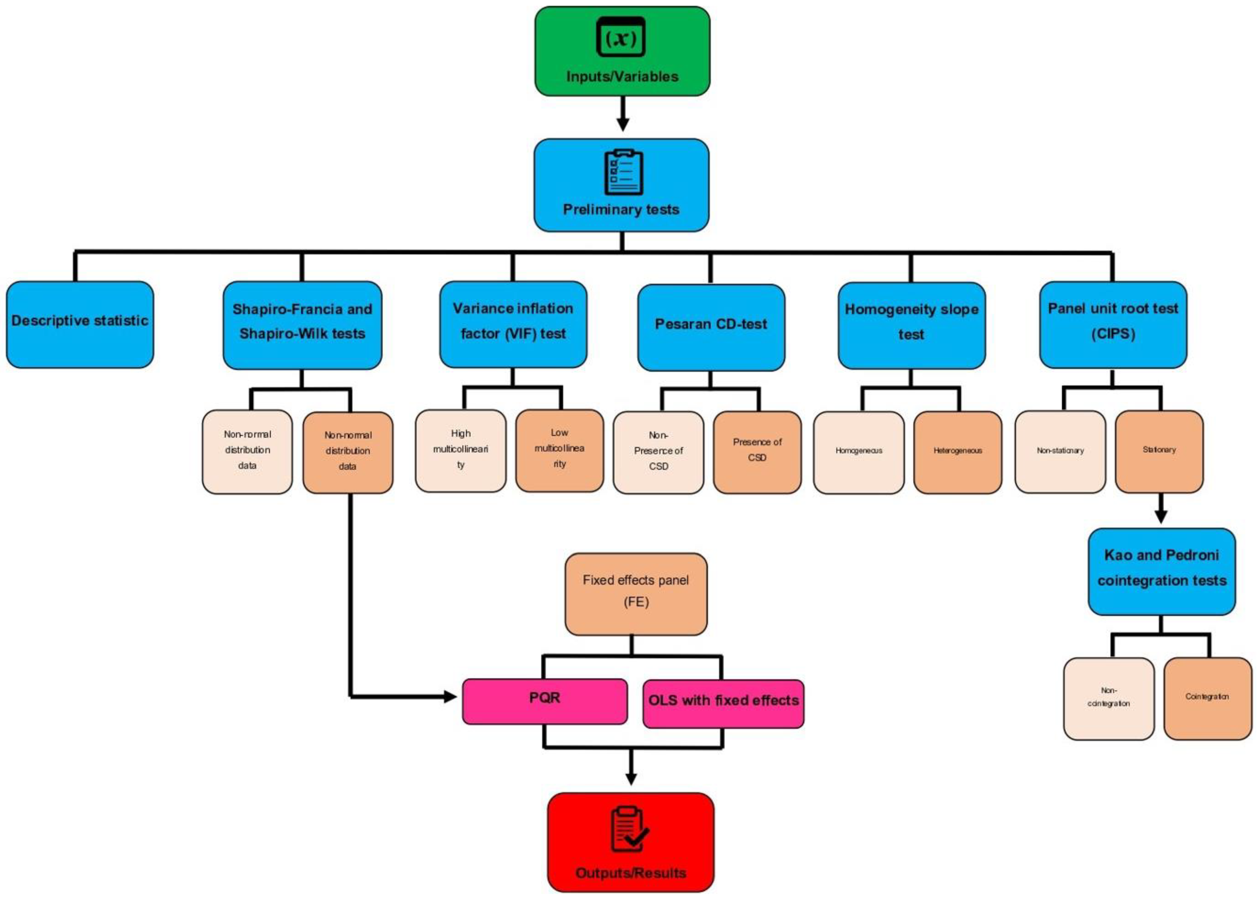
3.2. Method Approach

The method is divided into two parts: the first part explains the methodology related to the club’s convergence, and the second briefly deals with the quantile panel method. Indeed, to carry out this empirical investigation, the following methodological strategy will be used (see Figure 1 below).

3.2.1. The Club Convergence

The club convergence econometric method was created and introduced by Phillips and Sul [58]. This method, which the authors call the “log t-test”, allows the classification of countries into convergence groups or clubs. This method has numerous advantages over other existing convergence measures. For example, it is based on a time-varying and nonlinear factor model with the potential for transitional heterogeneity [59]. Furthermore, according to the club convergence hypothesis, convergence can only be achieved in groups of countries (or regions) with some common characteristics.

In this study, to examine the club convergence of the ecological footprint in global hectares (EFPG), a panel dataset at the country level is used, which is represented by the variable $X_{it}$, $i=1,\dots , N, t=1, \dots , T$, where N and T refer to the number of countries and periods, respectively. $X_{it}$ It is often decomposed into two components: Systematic $g_{it}$ and transient $a_{it}$ (Equation (1)).

$$X_{it}=g_{it}+a_{it}$$

(1)

The PS transforms Equation (1) so that the ordinary and distinct components in the panel are separated. Specifically, we decompose the $X_{it}$ panel data as follows (Equation (2)):

$$X_{it}=\left(\frac{g_{it}+a_{it}}{{\mu }_t}\right){\mu }_t={\delta }_{it}{\mu }_t. for all i,t$$

(2)

Thus, the variable $X_{it}$ has two components, common, ${\mu }_t$, and idiosyncratic, ${\delta }_{it}$. Both are time-varying. This formula makes the convergence test possible by testing whether the ${\delta }_{it}$ factor converges. To achieve this, PS defines the relative transfer parameter, $h_{it}$ (see Equation (3), below).

$$h_{it}=\frac{X_{it}}{\frac{1}{N}{\sum }_{i=1}^N{X}_{it}}=\frac{{\delta }_{it}}{\frac{1}{N}{\sum }_{i=1}^N{\delta }_{it}}$$

(3)

This transfer parameter shows the individual transfer path i concerning the panel average. This transfer path helps to obtain the cross-sectional variance of $h_{it}$ (see Equation (4), below).

$$H_t=\frac{1}{N}{\displaystyle \sum }_{i=n}^N{\left(h_{it}-1\right)}^2$$

(4)

The PS t-test is based on the idea that if $if {\delta }_{it}\to \mathsf{\delta } as t\to \infty then h_{it}\to 1$ and at the same time $H_t\to 0$, which guarantees convergence. PS shows that the transmission distance H_t has a finite shape (see Equation (5), below).

$$H_t~\frac{A}{L{\left(t\right)}^2{t}^{2\propto }} as t\to \infty$$

(5)

where A is a positive component, L(t) is a function that changes slowly and shows ∝ convergence speed. To test the Null convergence hypothesis (see Equation (6), below).

$$\begin{gathered} H_0:{\delta }_i=\delta and \alpha \ge 0 \\ {H}_A:{\delta }_i\ne \delta for all i. or \propto <0 \end{gathered}$$

(6)

We test this hypothesis with the regression model (see Equation (7), below).

$$\begin{gathered} \log \left(\frac{H_1}{H_t}\right)-2\log L\left(t\right)=a+b.\log \left(t\right)+{\epsilon }_t \\ For=\left[rT\right]. \left[rT\right]+1, \dots \dots T with r>0 \end{gathered}$$

(7)

Indeed, according to PS, $b=2a$ and r represent the fraction of the sample that should be discarded for regression analysis. The result of this regression is sensitive to the sample fraction r. Monte Carlo experiments show that r ∈ [0.2, 0.3] achieves good performance. It is recommended to set r = 0.3 for small or medium samples and r = 0.2 for large samples (T ≥ 100). Using the usual t-statistic for t_b, if $t_b<-$1.65 the null convergence hypothesis is rejected.

The identification of clubs in a panel is performed using the robust clustering algorithm method presented by [58] and is as follows:

• Sort countries based on their latest observations.
• Forming a Core Club, perform a statistical calculation of the tk convergence test for successive log(t) regressions based on the highest individuals k (2 ≤ k ≤ N) in the panel. Then, select the core size by maximizing tk with tb > −1.65.
• Add one country to the main group each time and estimate the log(t) regression in Equation (5). The decision on whether a country/territory should join the core group is based on the $\widehat{b}\le 0$ criteria.
• We repeat steps (b) and (c) for the remaining countries until we can no longer create a club, and each club has its convergence path. If the last group of the algorithm is not added, these countries form a divergent club.

3.2.2. The Panel Quantile Regression

The panel quantile regression (PQR) was introduced by Koenker and Bassett [60]. This model is based on a conditional quantitative function that minimizes the set of absolute error values in variables with asymmetric distributions. The advantage of quantile regression over ordinary least squares (OLS) is that it provides a comprehensive model by fitting multiple regression patterns to a dataset for different quantiles. This feature allows the inclusion of independent variables in all distribution parts, especially the initial and final quantiles. In addition, it does not face the limitations of conventional regression assumptions in estimating coefficients [61].

This model is a statistical method to calculate and plot different regression graphs and match different quantile points. While providing a complete and more comprehensive picture of the data, it allows the measuring of the relationship of independent variables with the desired quantiles of the dependent variable without the need for normal data even in the presence of outlier points. This regression is more powerful than the outlier data [62]. Quantile panel regression has been used in various fields (such as improving soil resources, economy, environment, climate, etc.) [29,63,64,65,66,67,68,69].

Therefore, this research applies the PQR method to evaluate the effect of ECI and EQ on the EFP. The mathematical formula of the PQR model is as follows in Equation (8).

$$\begin{gathered} y_i=x_i{b}_{\theta i}+{\mu }_{\theta i}. 0<\theta <1 \\ Quan{t}_{i\theta }\left(y_i/x_i\right)=x_i{\beta }_{\theta }, \end{gathered}$$

(8)

where x and y represent the vector of independent variables and the dependent variable, respectively; μ is a random error whose conditional quantile distribution is zero; $Quan{t}_{i\theta }\left(y_i/x_i\right)$ is the $\theta$th quantile of the explanatory variable; and the β_θ estimate shows the quantile regression θth and solves the Equation (9):

$$min{\displaystyle {\displaystyle \sum }_{yi\ge x_i^{\prime }\beta }}\theta \left|y_t-x_i^{\prime }\beta \right|+{\displaystyle \sum }_{yi<x_i^{\prime }\beta }\left(1-\theta \right)|y_t-x_i^{\prime }\beta |$$

(9)

As θ is equal to different values, different parameter estimations are obtained. The mean regression is a particular case of quantile regression under θ = 0.5 [70].

The model uses the logarithm form to remove the variables’ possible heterogeneity (Equation (10)).

$$\begin{gathered} LEFP{G}_{it}=La+{\beta }_{1}LPO{P}_{it}+{\beta }_{2}LGD{P}_{it}+{\beta }_{3}LEC{I}_{it}+{\beta }_{4}LNONRE{C}_{IT}+{\beta }_{5}LE{Q}_{it}+{\beta }_{6}LUR{B}_{it} \\ {\beta }_{7}LT{O}_{it}+{\delta }_{it.} \end{gathered}$$

(10)

where EFPG represents the ecological footprint measured in global hectares; POP is total population; GDP is Gross Domestic Product; ECI denotes economic complexity; NONREC is non-renewable energy consumption (which includes oil, gas, and coal) calculated in a million tonnes of oil equivalent; EQ is export quality; URB is urban population; and TO is trade openness.

Considering that the PQR model was used in this research to measure EFP, the quantile form of the equation is as follows (see Equation (11)):

$$\begin{gathered} Q_{\tau }\left(LEFP{G}_{it}\right)={(La)}_{\tau }+{\beta }_{1\tau }LPO{P}_{i\tau }+{\beta }_{2\tau }LGD{P}_{i\tau }+{\beta }_{3\tau }LEC{I}_{i\tau }+{\beta }_{4\tau }LNONRE{C}_{i\tau }+{\beta }_{5}LE{Q}_{it} \\ {\beta }_{6\tau }LUR{B}_{i\tau }+{\beta }_{7\tau }LT{O}_{i\tau }+{\delta }_{i\tau } \end{gathered}$$

(11)

In this regard, $Q_r$ means the estimation of the PQR $\tau th$ in the EFP and ${\left(la\right)}_r$ is the constant component. The coefficients ${\beta }_{1\tau },{\beta }_{2\tau },{\beta }_{3\tau },{\beta }_{4\tau },{\beta }_{5\tau }, {\beta }_{6\tau }, {\beta }_{7\tau }$ are the PQR parameters.

4. Empirical Results and Discussion

This section consists of two parts. In the first part, we check the convergence between countries using club convergence. Then, after selecting the convergent countries, we examine the effect of independent variables on the EFP using the PQR model.

4.1. Club Convergence Results

In this section, club convergence examines the convergence of the ecological footprint of 98 countries during the years 1990–2014. The results of this model are given in

Table 2. Results of the Ecological Footprint based on club convergence (98 countries).

Panel A: Club convergence tests		$\widehat{b}$ coef.	$t_{\widehat{b}}$
Full sample convergence	Countries	−0.4848	−34.5298 **
1st club	India, the United States of America, Brazil, and Canada	0.230	4.281
2nd club	Argentina, Australia, Italy, Egypt, Malaysia, France, Germany, Ghana, Indonesia, Japan, Mexico, South Africa, the United Kingdom, and South Korea	0.245	5.327
3rd club	Austria, Belgium, Bolivia, Cambodia, Cameroon, Chile, Colombia, Denmark, Ecuador, Finland, Gabon, Greece, Guatemala, Tanzania, Guinea, Israel, Singapore, Jordan, Kenya, Lebanon, Morocco, Portugal, Mozambique, the Netherlands, Oman, Peru, Poland, Qatar, Romania, Sri Lanka, Sweden, Switzerland, Spain, Tunisia, Venezuela, and Zambia	0.180	4.116
4th club	Costa Rica, Cuba, Djibouti, El Salvador, Haiti, Honduras, Hungary, Ireland, Paraguay, Liberia, Niger, Madagascar, Mauritania, New Zealand, Norway, Panama, Senegal, Sierra Leone, Philippines, and Somalia	0.227	6.310
5th club	Albania, Bhutan, Bulgaria, Burundi, Fiji, Gambia, Jamaica, Luxembourg, Myanmar, Nicaragua, North Korea, and Zimbabwe	0.123	5.140
6th club	Barbados, Malta, and Tonga	0.039	0.750
7th club	China and Cyprus	−0.878	−59.077 ***
Panel B: Club merging analysis		$\widehat{b}$ coef.	$t_{\widehat{b}}$
New club I	Merging Club 1 + 2	0.0554	1.3645
New club II	Merging Club 2 + 3	−0.1523	−4.7723 **
New club III	Merging Club 3 + 4	−0.0168	−0.5046
New club IV	Merging Club 4 + 5	0.0458	1.6717
New club V	Merging Club 5 + 6	−0.1970	−15.015 ***
New club VI	Merging Club 6 + 7	−0.7617	−291.984 ***
Panel C: Final club classifications		$\widehat{b}$ coef.	$t_{\widehat{b}}$
Club 1	Argentina, Brazil, Australia, Egypt, Canada, France, India, Indonesia, South Korea, Italy, Japan, Malaysia, Mexico, Germany, the United States, South Africa, and the United Kingdom	0.055	1.365
Club 2	Austria, Norway, Bolivia, Costa Rica, Cambodia, Belgium, Cameroon, Colombia, New Zealand, Denmark, Ecuador, Tanzania, El Salvador, Finland, Chile, Spain, Gabon, Greece, Guatemala, Guinea, Honduras, Ireland, Israel, Jordan, Kenya, Lebanon, Mauritania, Morocco, Mozambique, the Netherlands, Hungary, Oman, Panama, Romania, Paraguay, Peru, Poland, Portugal, Sri Lanka, Qatar, Senegal, Sweden, Singapore, Switzerland, Tunisia, Venezuela, and Zambia	−0.017	−0.505
Club 3	Albania, Bhutan, Bulgaria, Burundi, Fiji, Gambia, Jamaica, Luxembourg, Nicaragua, Niger, North Korea, Zimbabwe, Cuba, Sierra Leone, Haiti, and Liberia	0.123	5.140
Club 4	Barbados, Djibouti, Malta, Madagascar, Myanmar, Philippines, Somalia, and Tonga	0.039	0.750
Not convergent Group 5	China and Cyprus	−0.878	−59.077 **

Notes: For testing the one-sided null hypothesis: b ≥ 0 against b < 0, we use the critical value: t_0.05 = −1.651 in all cases; statistical significance at the (1%) and (5%) levels is denoted by *** and **, respectively, rejecting the null hypothesis of convergence.

. Therefore, in Panel A, the results of the overall convergence for all countries indicate that given $\left(t_{\widehat{b}}=-38.5298\right)$ is smaller than $t_{\widehat{b}}<-1.651$ and ($\widehat{b}=-0.4848)$ is smaller than $\widehat{b}<0$, the rejection of the null hypothesis demonstrates that there is a general convergence between all countries. Rejecting the null hypothesis for general convergence does not mean that there is no convergence in the subgroups. The result of the subgroup convergence test confirms the existence of seven subgroups and one non-convergent group. Of these seven groups, the first six are convergent among their group members, but the seventh group (China and Cyprus) is non-convergent. Convergence speed is measured by $\widehat{b}=2a$. As shown in Table 2 below, Panel A, Group 2, has the highest convergence speed.

However, in Panel B, we examine the integration of subgroups, showing that the integration of subgroups club 1 + 2, club 3 + 4, and club 4 + 5 are convergent. In addition, the integration rate in club 1 + 2 is faster than in other groups. Finally, in Panel C, we categorize the results of the final groups merging. The results of this section show four subgroups and one non-convergent group. All four subgroups are convergent. Finally, in this study, Group 2 in panel C, comprising 48 countries (e.g., Austria, Bolivia, Cambodia, Chile, Belgium, Cameroon, Colombia, Costa Rica, Denmark, Ecuador, Finland, Gabon, El Salvador, Greece, Guatemala, Guinea, Honduras, Hungary, Ireland, Israel, Jordan, Kenya, Mozambique, Lebanon, Mauritania, Morocco, New Zealand, Oman, the Netherlands, Panama, Norway, Peru, Paraguay, Poland, Portugal., Qatar, Romania, Senegal, Singapore, Spain, Sri Lanka, Sweden, Switzerland, Tanzania, Venezuela, Tunisia, and Zambia) is used to estimate the panel quantile regression model.

After identifying the convergence between groups of countries, the PQR model is used to investigate the effect of ECI and EQ on the EFP.

4.2. Panel Quantile Regression Results

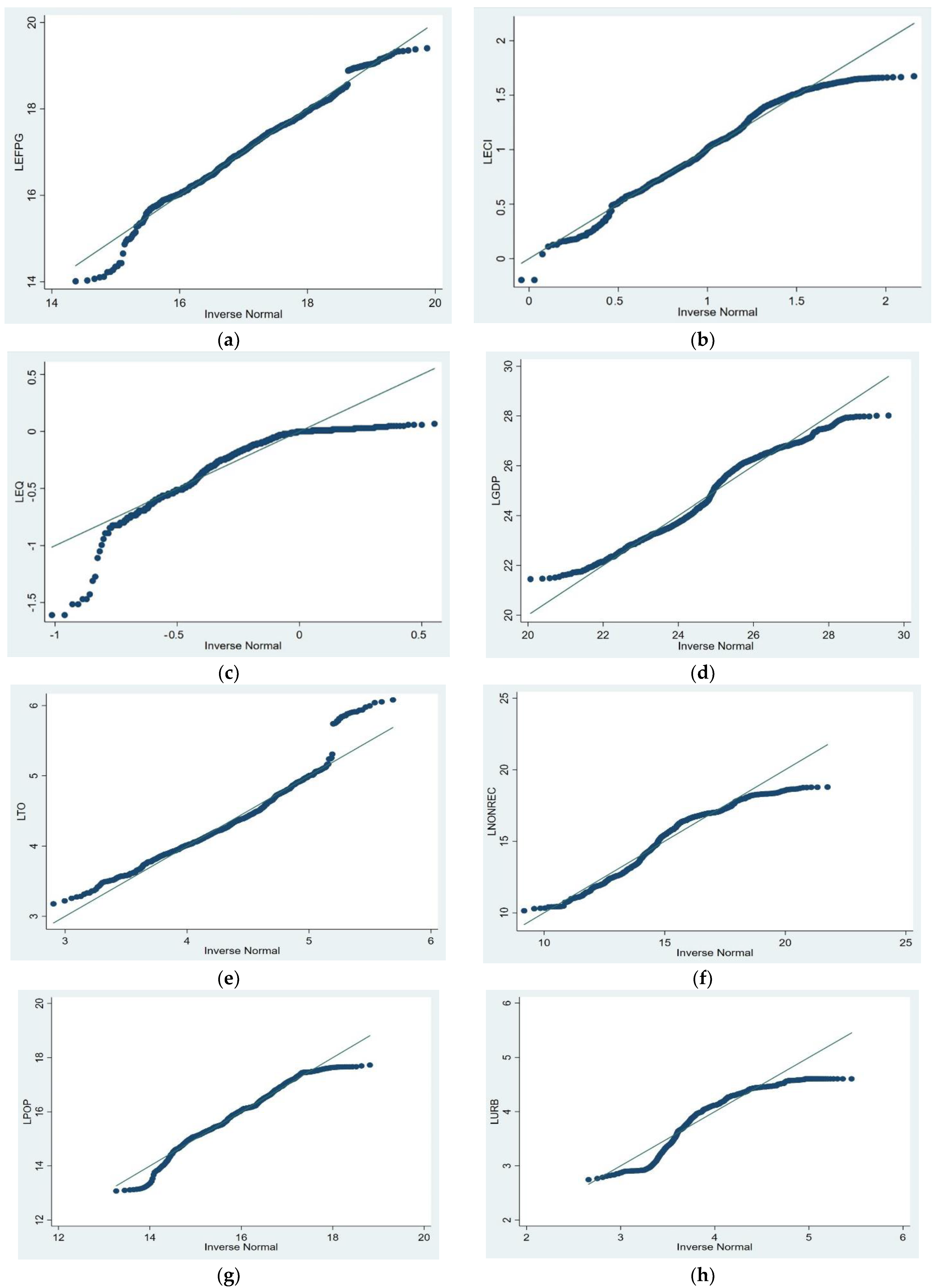
4.2.1. Pre-Estimation Tests

In this section, before performing the PQR model, we first examine the results of the preliminary testing, which include reading the normality (Royston [71]; Royston [72]), multicollinearity of the variables [73]; the existence of cross-sectional dependence [74]; the order of integration, i.e., unit roots [75]; and cointegration test [76,77]. Finally, the results of panel quantile regression estimation are given.

After selecting 48 countries based on the results of club convergence (see Table 2 above), we describe the statistics of the variables used in this study. In this context,

Table 3. Descriptive statistics.

Variables	Descriptive Statistics
	Obs.	Mean	Std.-Dev.	Min.	Max.
EFPG	1200	3.94 × 107	3.92 × 107	1216662	2.67 × 108
TO	1200	82.313	50.7916	23.98087	437.3267
EQ	1200	0.8165417	0.1739464	0.2	1.07
GDP	1200	1.59 × 1011	2.25 × 1011	2.06 × 109	1.47 × 1012
ECI	1200	3.053186	1.019706	0.8217199	5.32899
NONREC	1200	1.83 × 107	2.56 × 107	25313.77	1.44 × 108
POP	1200	1.31 × 107	1.10 × 107	476278	5.00 × 107
URB	1200	62.74421	22.13819	15.546	100

Notes: Obs. is the number of observations in the model, Std.-Dev. is the standard deviation, Min and Max are the minimum and maximum, respectively.

below shows the descriptive statistics of the variables.

After the descriptive statistics, panel quantile regression (PQR) was applied in this research. Therefore, the first test that should be checked is the normality of the data. Because the PQR method can be used when the data distribution is non-normal, in the normal distribution, there is no need to estimate with the PQR method, and the model can be estimated with OLS with fixed effects. In this research, two methods were used to check the data normality: (1) numerical method (see

Table 4. Normal distribution test.

Variables	Skewness	Kurtosis	Shapiro–Wilk Test		Shapiro–Francia Test		Obs
			Statistic		Statistic
LEFPG	−0.2046549	3.554171	0.98945	***	0.98966	***	1200
LTO	0.8929333	4.984875	0.95518	***	0.95518	***	1200
LEQ	−1.535696	6.753622	0.86400	***	0.86422	***	1200
LGDP	−0.35884	2.747878	0.96742	***	0.96836	***	1200
LECI	−0.331808	2.672438	0.97726	***	0.97778	***	1200
LNONREC	−0.581245	2.368702	0.94329	***	0.94420	***	1200
LPOP	−0.377437	3.302496	0.97973	***	0.98030	***	1200
LURB	−1.152019	3.569148	0.88414	***	0.88518	***	1200

Notes: *** denotes statistical significance at a (1%) level.

) and (2) graphical method (see Figure 2). In the numerical method, Shapiro–Francia [71] and Shapiro–Wilk [72] tests were applied to measure the normality. The results of the numerical method for both the Shapiro–Wilk and Shapiro–France tests show the non-normal distribution of the data. We also used skewness and kurtosis tests to check the normality of the data. If the skewness coefficient of the variable is equal to zero or its kurtosis coefficient is equal to three, the data normality is confirmed. According to Table 4, the skewness coefficient of all variables is non-zero, and their kurtosis coefficient is not close to 3. Therefore, it can be assured that it indicates the non-normal distribution of these variables. The results of both tests confirm the abnormal distribution of the variables.

Another way to show the normal distribution of data is to plot a graph. The Q-Q test graph is the most common method (Figure 2). If the Q-Q diagram corresponds to the straight blue line in Figure 2, it indicates the normal distribution of the data. Otherwise, the data distribution is not normal. As seen in Figure 2, the Q-Q graphs of all variables deviate from the straight line, which confirms the non-normal distribution of the data, and the PQR method can be used to estimate the model.

The next step is to explore multicollinearity using the Variance Inflation Factor (VIF) [73,78,79]. As can be seen (

Table 5. VIF, CSD, and HS tests.

Variables	VIF-Test		Cross-Sectional Dependence (CSD-Test)
	VIF	Mean VIF	CD Test	Corr	Abs (Corr)
EFPG	n.a.	2.31	79.34 ***	0.472	0.581
TO	1.54		58.91 ***	0.351	0.493
EQ	2.57		23.30 ***	0.139	0.387
GDP	3.26		155.50 ***	0.926	0.926
ECI	2.23		7.61 ***	0.045	0.393
NONREC	3.11		56.00 ***	0.339	0.649
POP	1.46		125.64 ***	0.748	0.957
URB	1.97		100.58 ***	0.634	0.825
Homogeneity Slope test
Models		Delta		Adjusted Delta
Model I		26.075 ***		28.305 ***

Notes: *** denotes statistical significance at the (1%) levels; n.a. denotes not available.

), the highest VIF value is related to GDP (3.26), and the lowest is POP (1.46). The average VIF value is also 2.31. The low value of VIFs shows no severe multicollinearity problem in the model. Then, the Pesaran CD-test [74] was applied to check the existence of cross-sectional dependence. The null hypothesis is cross-sectional independence. The results of the CD-test reject the null hypothesis for all variables, and the existence of cross-sectional dependence is confirmed. Finally, we check the homogeneity slope (HS) using the Pesaran and Yamagata [80] test. The null hypothesis is the existence of a homogeneous slope. According to the rejection of the null hypothesis, the results confirm the existence of a heterogeneous slope. The results of all three tests are given in Table 5.

The next test is to check the unit root for panel data. Considering the existence of cross-sectional dependence, Pesaran’s panel unit root test (CIPS) [75] is applied in this research. The null hypothesis of this test shows the existence of a panel unit root. As can be seen in

Table 6. Panel unit root test (CIPS).

CIPS			CIPS
Variables	Lags	(Zt-Bar)	Variables	Lags	(Zt-Bar)
EFPG	0	−1.165	LEFPG	0	−3.483 ***
	1	1.093		1	−0.537
TO	0	−1.218	LTO	0	−1.874 **
	1	−2.462		1	−3.257 ***
EQ	0	−5.871 ***	LEQ	0	−5.020 ***
	1	−3.855 **		1	−2.824 ***
GDP	0	7.423	LGDP	0	−1.161
	1	4.503		1	−2.349 ***
ECI	0	2.807	LECI	0	−1.119
	1	4.079		1	−2.469 ***
NONREC	0	4.158	LNONREC	0	−2.041 ***
	1	4.055		1	−2.483 ***
POP	0	5.117	LPOP	0	−1.408 **
	1	−8.005 ***		1	−7.868 ***
URB	0	−3.110 ***	LURB	0	−6.790 ***
	1	−2.113 **		1	−6.002 ***

Notes: “L” variables in the natural logarithms, ***, and ** denote statistical significance at the (1%) and (5%) levels, respectively.

, the results show that EFPG, TO, GDP, ECI, and NONREC variables at the level cannot reject the null hypothesis based on a unit root. However, EQ and URB with lags 1 and 2 and POP with lag 2 reject the null hypothesis at a (5%) significance level. However, after transferring the variables to a logarithmic form and performing the panel unit root test, the results indicate the stationary of all variables with lags of 1 or 2.

After confirming the stationary of all the variables in the logarithmic form, it is necessary to evaluate the long-term relationship between the variables in the next step. For this purpose, the cointegration test was applied [4,81]. In this study, the Kao [76], Pedroni [77], and Westerlund [82] cointegration tests were used to examine the long-term relationship between variables [83,84,85,86]. The null hypothesis in these tests shows the absence of cointegration. As seen in

Table 7. Kao, Pedroni, and Westerlund’s cointegration tests.

Kao Cointegration Test			Pedroni Cointegration Test
Estimators	t-Statistic	Prob.	Estimators	t-Statistic	Prob.
ADF	−5.3062	0.0000 ***	Modified Phillips–Perron t	7.0314	0.0000 ***
Residual variance	0.00164		Phillips–Perron t	−11.9530	0.0000 ***
HAC variance	0.00135		Augmented Dickey-Fuller t	−10.6734	0.0000 ***
Westerlund panel cointegration test
Statistic	Value		Z-value	Robust p−value
Gt	−2.426		0.139	0.002	***
Ga	−6.664		5.690	0.041	**
Pt	−14.757		1.557	0.080	*
Pa	−4.228		5.892	0.140

Notes: ***, **, and * are used to denote statistical significance at the (1%), (5%), and (10%) levels, respectively.

, the cointegration test results for the Pedroni, Kao, and Westerlund tests indicate the null hypothesis rejection and the existence of a long-term relationship between EFP and explanatory variables.

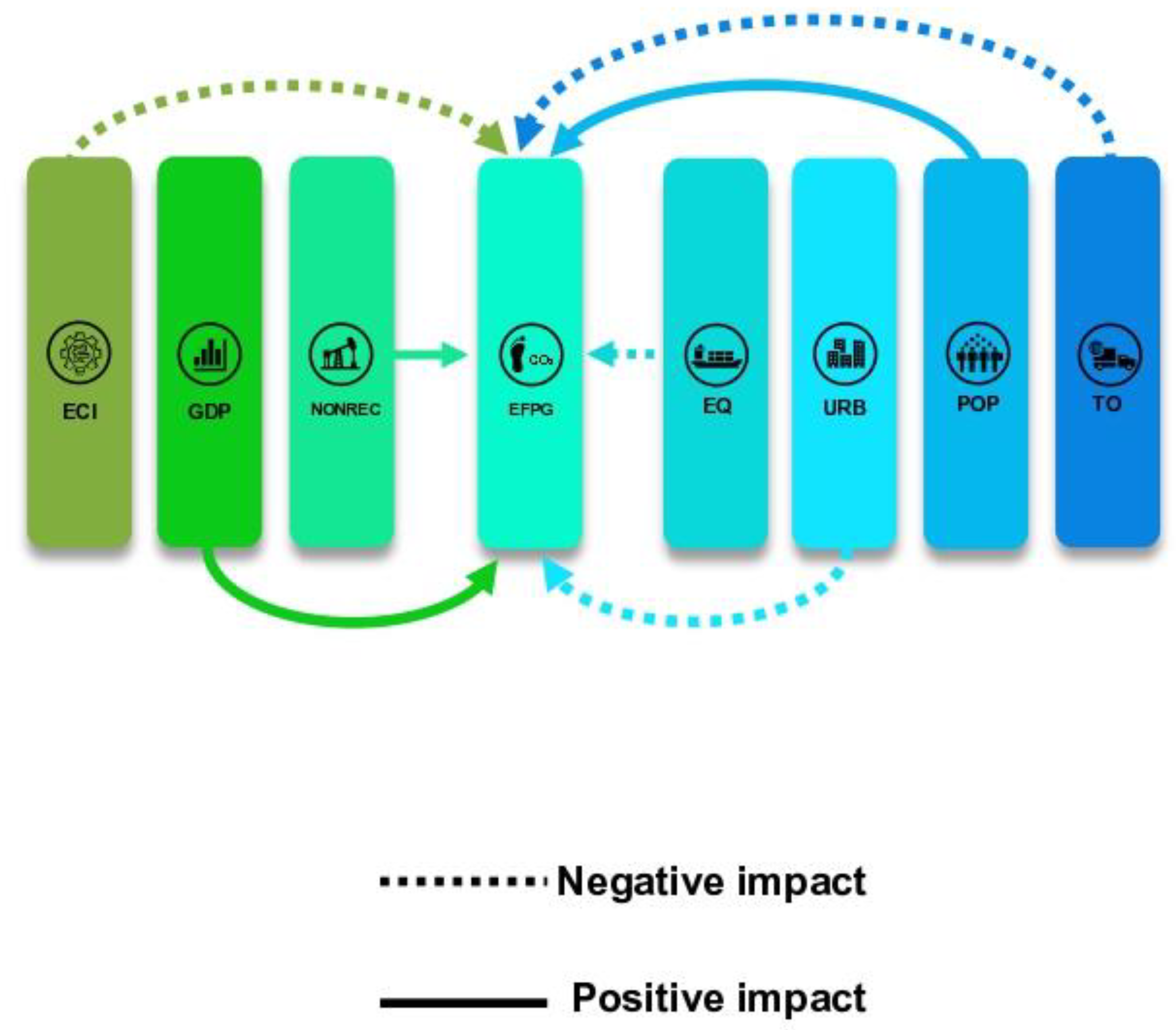
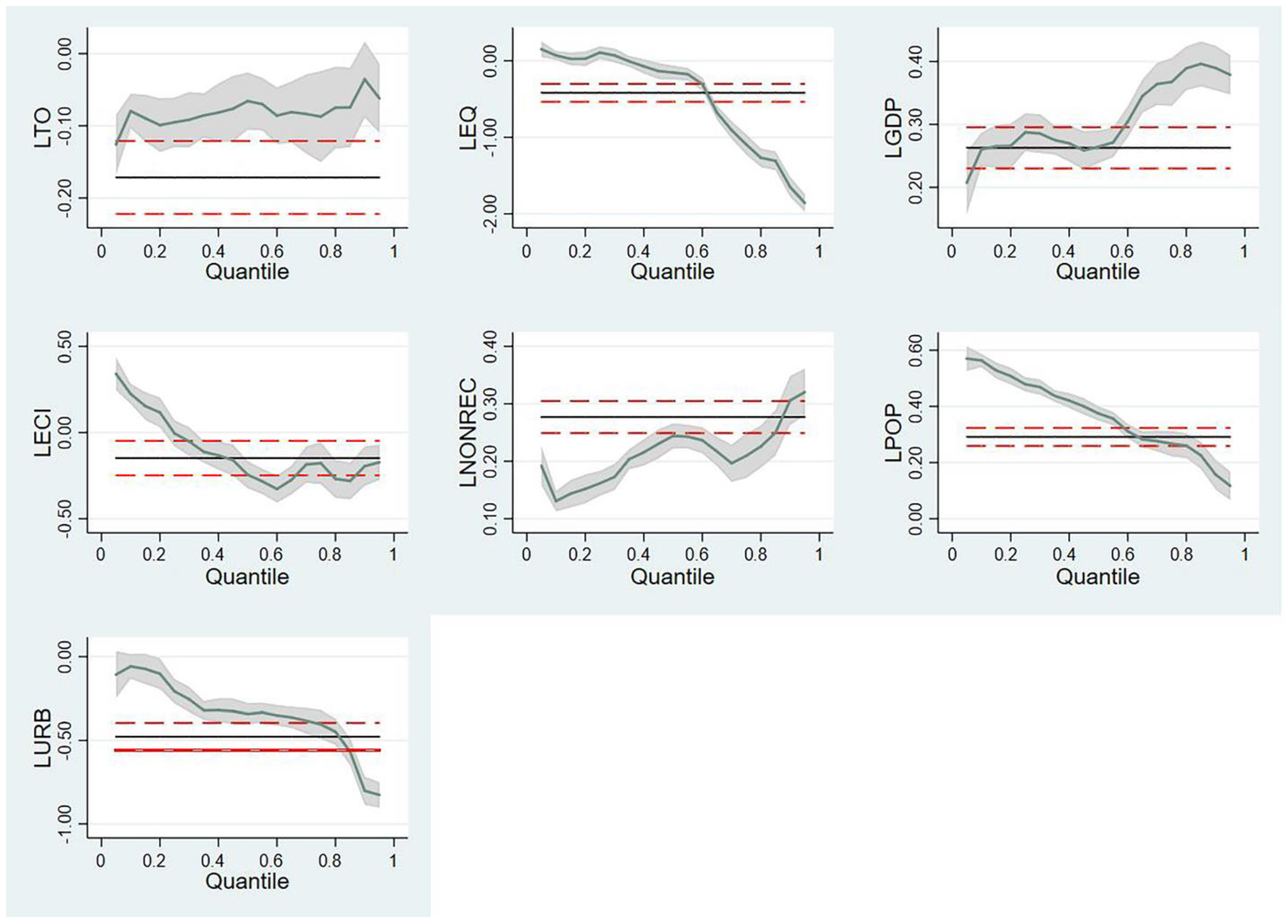
4.2.2. Panel Quantile Regression Result and Discussion

After conducting the preliminary tests, it is time to estimate the PQR model. We applied 10th, 25th, 50th, 75th, and 90th quantiles for calculation. Therefore, before assessing the model, we first divide the countries based on EFP into six groups related to these quantiles (see

Table 8. Country distribution of ecological footprint (gha).

Quantile	Country
$\mathrm{quantile} <10\mathrm{th}$	Gabon, Mauritania, Panama, and Costa Rica
$10\mathrm{th}\le \mathrm{quantile} <25\mathrm{th}$	Zambia, El Salvador, Jordan, Honduras, Guinea, Cambodia, Senegal, and Lebanon
$25\mathrm{th}\le \mathrm{quantile} <50\mathrm{th}$	Mozambique, Cameroon, Tunisia, Madagascar, Paraguay, Guatemala, Sri Lanka, New Zealand, Bolivia, Ireland, Ecuador, and Singapore
$50\mathrm{th}\le \mathrm{quantile} <75\mathrm{th}$	Oman, Norway, Finland, Israel, Kenya, Hungary, Qatar, Switzerland, Morocco, Denmark, Portugal, and Tanzania
$75\mathrm{th}\le \mathrm{quantile} <90\mathrm{th}$	Austria, Peru, Sweden, Chile, Greece, Romania, Belgium, and Venezuela
$\mathrm{quantile}\ge 90\mathrm{th}$	Colombia, the Netherlands, Poland, and Spain

Notes: According to the level of EFP, we divided the panel of 48 countries into six grades.

) below.

Table 9. Estimation results from the PQR model and panel fixed effects.

Variables	Quantiles										OLS
	10th		25th		50th		75th		90th		Fixed Effects
LTO	−0.0790	***	−0.0950	***	−0.066	**	−0.0872	**	−0.0356		−0.1775	***
LEQ	0.0700		0.1074		−0.154	***	−1.0933	***	−1.6452	***	−0.4141	***
LGDP	0.2603	***	0.2875	***	0.2646	***	0.3675	***	0.3897	***	0.2619	***
LECI	0.2243	***	−0.005		−0.245	***	−0.1779	**	−0.1949	**	−0.1476	***
LNONREC	0.1306	***	0.1617	***	0.2441	***	0.2095	***	0.3059	***	0.2774	***
LPOP	0.5836	***	0.4787	***	0.3750	***	0.2670	***	0.1575	***	0.2899	***
LURB	−0.5802	*	−0.207	***	−0.342	***	−0.4041	***	−0.8012	***	−0.4779	**
Constant	−0.3712		−0.207	***	1.6245	***	1.6225	***	1.8114	***	1.4410	***
Pseudo R2	0.9312		0.8831		0.8802		0.8519		0.8689		0.8661

Notes: ***, **, and * denote statistical significance at the (1%), (5%), and (10%) levels, respectively; “L” denotes variables in natural logarithms.

shows the results of PQR and OLS estimation with fixed effects. The OLS estimator with fixed effects is used to check the robustness of the model. The results of this model are compared with the 50th quantile.

A figure was created to summarise the effect of independent variables on the dependent ones (see Figure 3 below) to facilitate the visualisation of results found in Table 9 above.

After showing the summary of the effects, it is necessary to present the discussions and the possible explanations for the results found. As shown in Table 9, except in the 90th quantile, at other levels of quantiles, trade openness has a significant negative effect on the EFP, which means that increasing the volume of trade in these countries reduces the EFP. The results of Sbia et al. [87] confirm that trade openness improves the quality of the environment by transferring advanced and environmentally friendly technologies instead of using older technologies heavily dependent on fossil consumption. In a study of newly industrialised countries, Ahmed et al. [88] stated that open trade openness improves the quality of the environment. Aşıcı and Acar [89] also found in a study of 116 countries on the EFP that trade openness reduces environmental degradation. Zhang et al. [38], Baek et al. [90], and Frankel and Rose [91] confirmed the results. At the same time, some other studies reported opposite results. In a survey of the organisation of Islamic cooperation (OIC) countries, Ali et al. [92] said that open trade increases the EFP. Al-Mulali et al. [93] also found in a study of 58 developing and developed countries that open trade increases the EFP. In a survey of 98 countries, Le et al. [94] stated that trade openness increases particulate matter (PM₁₀) emissions.

Export quality in the EFP’s 50th, 75th, and 90th quantiles is negative and significant. The results show that this effect is greater at higher quantile levels, which means that the EFP decreases more with increasing export quality. Empirical results show that increasing the variety and quality of export products helps to improve the quality of the environment through increasing the ability to provide environmentally friendly technologies. Research findings by Doğan et al. [19] for 63 developed and developing countries confirm that trade quality reduces CO₂ emissions. Gozgor and Can [9] also confirm the research findings in a study for China, and they stated that trade quality decreases CO₂ emissions. Murshed and Dao [20] also found in a study of selected South Asian economies (e.g., Sri Lanka, Pakistan, Bangladesh, India, and Nepal) that improving export quality would reduce CO₂ emissions. Li et al. [50], in a study for China, found that by increasing export diversification, CO₂ emissions decrease, which helps to improve the quality of the environment.

In contrast, other studies have reported a positive relationship between export quality and environmental degradation. Wang et al. [48] studied the top ten renewable energy countries, and the top ten ECIs indicate that trade quality positively affects CO₂ emissions. The results of studies by Fang et al. [17] for 82 developing nations also show that export quality increases CO₂ emissions. Research findings for ten newly industrialised countries performed by Can et al. [95] indicate that export product diversification increases CO₂ emissions. The study by Shahzad et al. [96] for 63 developed and developing countries confirms that export product diversification reduces CO₂ emissions. The findings of Hu et al. [97] for 35 developed and 93 developing countries indicate that export product diversification negatively and positively impacts CO₂ emissions in developed and developing countries, respectively.

As expected, the effect of GDP on EFP is positive and significant in all quantiles. This effect is greater in higher quantiles. So that a (1%) increase in GDP in the 90th quantile causes a (0.3897%) increase in EFP. The study results of Hassan et al. [33] for Pakistan are consistent with this study’s findings. They reported that economic growth increases the EFP. In a survey of five European Union (EU) countries (e.g., Spain, Germany, Italy, France, and the United Kingdom), Balsalobre-Lorente et al. [98] confirmed that economic growth would increase CO₂ emissions. Saud et al. [99], in a study for 59 Belt and Road Initiative (BRI) countries, confirmed that economic growth causes environmental degradation. Some other studies also confirm the research findings [32,37,100]. The results of Hanif [101] for sub-Saharan Africa showed an inverse U-shape relationship between economic growth and CO₂ emissions. Sarkodie’s [102] study to investigate the effect of economic growth on environmental degradation in 17 African countries confirms the EKC hypothesis. In separate research, Haseeb et al. [103] and Alam et al. [104] demonstrate the EKC hypothesis.

The results of ECI on ecological footprint indicate that in the 10th quantile, ECI has a positive and significant effect on EFP. In contrast, the ECI on 50th, 75th, and 90th quantiles negatively and significantly affect EFP. It can be said that the low level of technology leads to the use of products with high energy consumption, which in turn leads to an increase in the EFP. In contrast, with the rise in ECI, newer and environmentally friendly technologies are being used. Moreover, this reduces the EFP. The empirical results indicate that economic complexity has asymmetric effects on the environment at the level of different quantiles. So, experimental results from a critical point of view show that production and economic structures significantly affect the environment. The findings of Kazemzadeh et al. [35] for 25 countries using the QPR model are consistent with the results of this study. They stated that low ECI increases environmental degradation, while the high quantile level of ECI helps to improve environmental quality. Findings from Doğan et al. [46] for 28 OECD countries show that ECI can help reduce environmental degradation. In a study for France, Can and Gozgor [51] confirmed that high levels of ECI reduce CO₂ emissions. Ahmed et al. [105], in a study of countries G7, found that increasing ECI causes a decrease in the ecological footprint.

In comparison, some other studies have reported a positive relationship between ECI and environmental degradation. The findings of Can et al. [95] for newly industrialized countries showed that ECI increases CO₂ emissions. The study results by Yilanci and Pata [34] for China indicate that ECI increases the ecological footprint. Doğan et al. [106], in a study of 55 countries, stated that the ECI of environmental degradation has increased in low and high-middle-income countries and has controlled CO₂ emissions in high-income countries. Rafei et al. [52], in a study of countries with different institutional qualities, discovered that increasing ECI significantly affects the ecological footprint. Shahzad et al. [53] found that increasing economic complexity increases the ecological footprint of the United States.

The results of Table 9 also show that urbanisation at all quantiles has a significant negative effect on the EFP, which is more significant at higher levels. So that (1%) increase in urbanisation causes a (0.8012%) increase in EFP. The findings of Lv and Xu [107] for 55 middle-income countries confirm the results of this study. They reported that urbanisation reduces CO₂ emissions. In a study of 19 emerging economies, Saidi and Mbarek [108] stated that urbanisation improves environmental quality. Sharma [109], in a survey of 69 countries, divided them into three sub-panel based on income level: high income, medium income, and low income found that in all three categories, urbanisation reduces CO₂ emissions.

In contrast, some other studies have identified urbanisation as one of the factors of environmental degradation. Parikh and Shukla’s [110] results for 83 countries indicate that urbanisation increases CO₂ emissions. Findings by Wang et al. [111] for the Association of Southeast Asian Nations (ASEAN) countries confirm that urbanisation increases CO₂ emissions. Wang and Dong [112], in a study of 14 sub-Saharan Africa (SSA) countries during 1990–2014, stated that urbanisation increases the ecological footprint. In addition, the PQR results are shown graphically in Figure 4.

4.2.3. Robustness Check

It is necessary to check the model’s robustness [113] to gauge its validity. For this purpose, we used three methods: (i) the robust regression estimator (MM-Estimation), (ii) fully modified ordinary least squares (FMOLS), and (iii) the dynamic ordinary least squares (DOLS) to check the robustness of the main model. If the coefficients’ direction and significance do not change, the model’s results can be trusted. The results of the robustness check of the model are given in

Table 10. Robustness check.

Variables	DOLS	FMOLS	MM-Estimation
LTO	−0.0344 **	−0.0221 **	−0.0627 ***
LEQ	−0.0163 ***	−0.0102 ***	−0.0265 **
LGDP	0.3548 ***	0.3278 ***	0.2796 ***
LECI	−0.2338 ***	−0.2660 ***	−0.1336 **
LNONREC	0.2264 ***	0.2406 ***	0.1341 ***
LPOP	0.2498 ***	0.1877 ***	0.5035 ***
LURB	−0.4917 ***	−0.4164 ***	−0.1509 ***
Constant			2.4329 ***
R2	0.9250	0.9198	0.9384

Notes: *** and ** denote statistical significance at the (1%), and (5%) levels, respectively.

.

As can be seen in Table 10, the results of the model’s robustness show that the effect of the variables (signs) and their significance on the ecological footprint are the same as in the original model. Therefore, the main model is reliable and can be used for analysis.

5. Conclusions and Policy Implications

A two-step approach was used to research the impact of economic complexity and export quality on ecological footprint. First, club convergence was applied to identify the countries that follow a similar convergence path. Second, the econometric technique of panel quantile regression was used to determine the explanatory power of two variables, economic complexity, and export quality on the ecological footprint.

Data cover the period from 1990 to 2014. Therefore, this option matches the period for which the variables are available for all countries in this panel. The club convergence method was used in 98 countries based on the ecological footprint variable. The research revealed four groups of convergent countries and one group that was not convergent. Therefore, from the 98 countries analysed, we chose to research the most numerous clubs (48 countries).

The panel quantile approach was used because of the linkage between the ecological footprint (explained variable), the trade openness, export quality index, GDP, economic complexity index, non-renewable energy consumption, the urban population as a percentage of the total population, and total population (explanatory variables) revealed to be nonlinear.

Gross Domestic Product, non-renewable energy consumption, and population damage the environment as they aggravate the ecological footprint, regardless of the quantity considered. Nevertheless, the environmental damage becomes less pronounced as we increase the quantiles. Urbanisation contributes to reducing the ecological footprint for all quantiles. It was found that export quality and trade openness lower the ecological footprint but not in all estimated quantiles. Trade openness losses the capacity to reduce footprint at the 90th quantile. Export quality becomes a reducer of footprint at quantile 50th or upper, and at upper quantiles, its contribution to reducing footprint is vast. Economic complexity reveals mixed results. Aggravate the ecological footprint in low quantile (10th), become not statistically significant at quantile 25th, and reduce the ecological footprint in upper quantiles.

The limitation of ecological footprint damage involves a wide range of policy actions. First, policymakers must recognize the effect of economic and social variables, such as consumption, on the ecological footprint. Therefore, policymakers must go further regarding the structure of their economies and promote less damaging consumption and production. Second, policymakers must promote energy policies encouraging the deployment of energy-efficient sources and accelerating the energy transition to renewable sources. These actions contribute to mitigating the ecological footprint damage. Finally, policymakers must implement measures to circumvent the population growth as it exerts an additional burden on the ecological footprint damage.

The tentative findings of this research are valuable for expanding the literature and have particular consequences for improving the policies of complex economies that have diversified export sectors and are confronted with the necessity to reduce environmental degradation. Moreover, these findings can help to develop new policies of using clean energy, reducing energy consumption, and achieving sustainable development.

The study also reveals that analysing countries with similar convergence processes can be a criterion for better identifying the factors that influence the ecological footprint. Thus, the next step should investigate the relationships between the variables in different convergence processes. However, the short period of data available imposes some limitations on our research. Therefore, further improvements in research can take advantage of econometric approaches that disentangle the total impact on its temporal dimensions, i.e., the short and long-term impacts. Furthermore, research should evolve to assess developing and developed countries’ distinctions.

It should be stressed that the conclusions of this research are probably valid only for countries that share similar patterns of convergence in their ecological footprint. Moreover, the generalization of results could be poor in the presence of relationships that are not linear in their behaviours, as is the case of possible sudden changes in the environmental situation.

References

1. Bhattacharya, M.; Churchill, S.A.; Paramati, S.R. The dynamic impact of renewable energy and institutions on economic output and CO2 emissions across regions. Renew. Energy 2017, 111, 157–167. [Google Scholar] [CrossRef]
2. Apergis, N.; Can, M.; Gozgor, G.; Lau, C.K.M. Effects of export concentration on CO2 emissions in developed countries: An empirical analysis. Environ. Sci. Pollut. Res. 2018, 25, 14106–14116. [Google Scholar] [CrossRef]
3. Acheampong, A.O. Economic growth, CO2 emissions and energy consumption: What causes what and where? Energy Econ. 2018, 74, 677–692. [Google Scholar] [CrossRef]
4. Al-Mulali, U.; Ozturk, I. The investigation of environmental Kuznets curve hypothesis in the advanced economies: The role of energy prices. Renew. Sustain. Energy Rev. 2016, 54, 1622–1631. [Google Scholar] [CrossRef]
5. Ozcan, B.; Apergis, N.; Shahbaz, M. A revisit of the environmental Kuznets curve hypothesis for Turkey: New evidence from bootstrap rolling window causality. Environ. Sci. Pollut. Res. 2018, 25, 32381–32394. [Google Scholar] [CrossRef]
6. Rahman, S.U.; Chen, S.; Saud, S.; Saleem, N.; Bari, M.W. Nexus between financial development, energy consumption, income level, and ecological footprint in CEE countries: Do human capital and biocapacity matter? Environ. Sci. Pollut. Res. 2019, 26, 31856–31872. [Google Scholar] [CrossRef]
7. Germani, A.R.; Ker, A.P.; Castaldo, A. On the existence and shape of an environmental crime Kuznets Curve: A case study of Italian provinces. Ecol. Indic. 2020, 108, 105685. [Google Scholar] [CrossRef]
8. Arango-Miranda, R.; Hausler, R.; Romero-López, R.; Glaus, M.; Pasillas-Díaz, J.R. Testing the Environmental Kuznets Curve Hypothesis in North America’s Free Trade Agreement (NAFTA) Countries. Energies 2020, 13, 3104. [Google Scholar] [CrossRef]
9. Gozgor, G.; Can, M. Does export product quality matter for CO2 emissions? Evidence from China. Environ. Sci. Pollut. Res. 2017, 24, 2866–2875. [Google Scholar] [CrossRef]
10. Chen, W.; Lei, Y. The impacts of renewable energy and technological innovation on environment-energy-growth nexus: New evidence from a panel quantile regression. Renew. Energy 2018, 123, 1–14. [Google Scholar] [CrossRef]
11. Onafowora, O.A.; Owoye, O. Bound testing approach to analysis of the environment Kuznets curve hypothesis. Energy Econ. 2014, 44, 47–62. [Google Scholar] [CrossRef]
12. Kasman, A.; Duman, Y.S. CO2 emissions, economic growth, energy consumption, trade and urbanization in new EU member and candidate countries: A panel data analysis. Econ. Model. 2015, 44, 97–103. [Google Scholar] [CrossRef]
13. Wang, Z.; Liu, W. Determinants of CO2 emissions from household daily travel in Beijing. China: Individual Travel Characteristic Perspectives. Appl. Energy 2015, 158, 292–299. [Google Scholar] [CrossRef]
14. Paramati, S.R.; Ummalla, M.; Apergis, N. The effect of foreign direct investment and stock market growth on clean energy use across a panel of emerging market economies. Energy Econ. 2016, 56, 29–34. [Google Scholar] [CrossRef]
15. Doğan, E.; Turkekul, B. CO2 emissions, real output, energy consumption, trade, urbanization and financial development: Testing the EKC hypothesis for the USA. Environ. Sci. Pollut. Res. 2016, 23, 1203–1213. [Google Scholar] [CrossRef]
16. Albulescu, C.; Tiwari, A.K.; Yoon, S.-M.; Kang, S.H. FDI, income, and environmental pollution in Latin America: Replication and extension using panel quantiles regression analysis. Energy Econ. 2019, 84, 104504. [Google Scholar] [CrossRef]
17. Fang, J.; Gozgor, G.; Lu, Z.; Wu, W. Effects of the export product quality on carbon dioxide emissions: Evidence from developing economies. Environ. Sci. Pollut. Res. 2019, 26, 12181–12193. [Google Scholar] [CrossRef]
18. Pata, U.K. Renewable and nonrenewable energy consumption, economic complexity, CO2 emissions, and ecological footprint in the USA: Testing the EKC hypothesis with a structural break. Environ. Sci. Pollut. Res. 2020, 28, 846–861. [Google Scholar] [CrossRef]
19. Doğan, B.; Madaleno, M.; Tiwari, A.K.; Hammoudeh, S. Impacts of export quality on environmental degradation: Does income matter? Environ. Sci. Pollut. Res. 2020, 27, 13735–13772. [Google Scholar] [CrossRef]
20. Murshed, M.; Dao, N.T.T. Revisiting the CO2 emission-induced EKC hypothesis in South Asia: The role of Export Quality Improvement. GeoJournal 2020, 87, 535–563. [Google Scholar] [CrossRef]
21. Shahbaz, M.; Mahali, M.K.; Shah, S.H.; Sato, J.R. Time-varying analysis of CO2 emissions, energy consumption, and economic growth Nexus: Statistical experience in next 11 countries. Energy Policy 2016, 98, 33–48. [Google Scholar] [CrossRef]
22. Neagu, O. Economic Complexity and Ecological Footprint: Evidence from the Most Complex Economies in the World. Sustainability 2020, 12, 31. [Google Scholar] [CrossRef]
23. Lin, D.; Hanscom, L.; Martindill, J.; Borucke, M.; Cohen, L.; Galli, A.; Lazarus, E.; Zokai, G.; Iha, K.; Eaton, D. Working Guidebook to the National Footprint and Biocapacity Accounts; Global Footprint Network: Oakland, CA, USA, 2020; Available online: http://www.footprintnetwork.org (accessed on 1 August 2022).
24. Nijkamp, P.; Rossi, E.; Vindigni, G. Ecological footprints in plural: A meta-analytic comparison of empirical results. Reg. Stud. 2004, 38, 747–765. [Google Scholar] [CrossRef]
25. Al-Mulali, U.; Ozturk, I.; Lean, H.H. The influence of economic growth, urbanization, trade openness, financial development, and renewable energy on pollution in Europe. Nat. Hazards 2015, 79, 621–644. [Google Scholar] [CrossRef]
26. Mrabet, Z.; Alsamara, M. Testing the Kuznets curve hypothesis for Qatar: A comparison between carbon dioxide and ecological footprint. Energy Rev. 2017, 70, 1366–1375. [Google Scholar] [CrossRef]
27. Destek, M.A.; Ulucak, R.; Doğan, E. Analyzing the environmental Kuznets curve for the EU countries: The role of ecological footprint. Environ. Sci. Pollut. Res. 2018, 25, 29387–29396. [Google Scholar] [CrossRef]
28. Gómez, M.; Rodríguez, J.C. Analysis of the environmental Kuznets curve in the NAFTA Countries. EconoQuantum 2020, 17, 57–79. [Google Scholar] [CrossRef]
29. Gómez, M.; Rodríguez, J.C. The Ecological Footprint and Kuznets Environmental Curve in the USMCA Countries: A Method of Moments Quantile Regression Analysis. Moments Quantile Regression Analysis. Energies 2020, 13, 6650. [Google Scholar] [CrossRef]
30. Charfeddine, L.; Mrabet, Z. The impact of economic development and social-political factors on ecological footprint: A panel data analysis for 15 MENA countries. Renew. Sustain. Energy Rev. 2017, 76, 138–154. [Google Scholar] [CrossRef]
31. Alola, A.A.; Bekun, F.V.; Sarkodie, S.A. Dynamic impact of trade policy, economic growth, fertility rate, renewable and nonrenewable energy consumption on ecological footprint in Europe. Sci. Total. Environ. 2019, 685, 702–709. [Google Scholar] [CrossRef]
32. Chen, Y.; Wang, Z.; Zhong, Z. CO2 emissions, economic growth, renewable and nonrenewable energy production and foreign trade in China. Renew. Energy 2019, 131, 208–216. [Google Scholar] [CrossRef]
33. Danish Hassan, S.T.; Baloch, M.A.; Mahmood, N.; Zhang, J.W. Linking economic growth and ecological footprint through human capital and biocapacity. Sustain. Cities Soc. 2019, 47, 101516. [Google Scholar] [CrossRef]
34. Yilanci, V.; Pata, U.K. Investigating the EKC hypothesis for China: The role of economic complexity on ecological footprint. Environ. Sci. Pollut. Res. 2020, 27, 32683–32694. [Google Scholar] [CrossRef]
35. Kazemzadeh, E.; Fuinhas, J.A.; Koengkan, M. The impact of income inequality and economic complexity on ecological footprint: An analysis covering a long-time span. J. Environ. Econ. Policy 2021, 11, 133–153. [Google Scholar] [CrossRef]
36. World Bank Data (WBD). Available online: https://databank.worldbank.org/home (accessed on 23 July 2022).
37. Raza, S.A.; Shah, N. Testing environmental Kuznets curve hypothesis in G7 countries: The role of renewable energy consumption and trade. Environ. Sci. Pollut. Res. 2018, 25, 26965–26977. [Google Scholar] [CrossRef]
38. Zhang, S.; Liu, X.; Bae, J. Does trade openness affect CO2 emissions: Evidence from ten newly industrialized countries? Environ. Sci. Pollut. Res. 2017, 24, 17616–17625. [Google Scholar] [CrossRef]
39. Shahbaz, M.; Shafiullah, M.; Mahalik, M.K. The dynamics of financial development, globalisation, economic growth, and life expectancy in sub-Saharan Africa. Aust. Econ. Pap. 2019, 58, 444–479. [Google Scholar] [CrossRef]
40. Can, M.; Gozgor, G. Effects of export product diversification on quality upgrading: An empirical study. J. Int. Trade Econ. Dev. 2018, 27, 293–313. [Google Scholar] [CrossRef]
41. Rafindadi, A.A. Does the need for economic growth influence energy consumption and CO2 emissions in Nigeria? Evidence from the innovation accounting test. Renew. Sustain. Energy Rev. 2016, 62, 1209–1225. [Google Scholar] [CrossRef]
42. Gozgor, G.; Can, M. Export product diversification and the environmental Kuznets curve: Evidence from Turkey. Environ. Sci. Pollut. Res. 2016, 23, 21594–21603. [Google Scholar] [CrossRef]
43. Moghadam, H.E.; Dehbashi, V. The impact of financial development and trade on environmental quality in Iran. Empir. Econ. 2018, 54, 1777–1799. [Google Scholar] [CrossRef]
44. Neagu, O. The Link between Economic Complexity and Carbon Emissions in the European Union Countries: A Model Based on the Environmental Kuznets Curve (EKC) Approach. Sustainability 2019, 11, 4753. Available online: https://www.mdpi.com/2071-1050/11/17/4753/htm (accessed on 23 July 2022). [CrossRef]
45. Lapatinas, A.; Garas, A.; Boleti, E.; Kyriakou, A. Economic Complexity and Environmental Performance: Evidence from A World Sample. 2019. Available online: https://mpra.ub.uni-muenchen.de/92833/1/MPRA_paper_92833.pdf (accessed on 1 August 2022).
46. Doğan, B.; Driha, O.M.; Balsalobre-Lorente, D.; Shahzad, U. The mitigating effects of economic complexity and renewable energy on carbon emissions in developed countries. Sustain. Dev. 2021, 29, 1–12. [Google Scholar] [CrossRef]
47. Hausmann, R.; Hidalgo, C.A.; Bustos, S.; Coscia, M.; Simoes, A.; Yildirim, M.A. The Atlas of Economic Complexity: Mapping Paths to Prosperity; MIT Press: Cambridge, MA, USA, 2014. [Google Scholar]
48. Wang, Z.; Jebli, M.B.; Madaleno, M.; Doğan, B.; Shahzad, U. Does export product quality and renewable energy induce carbon dioxide emissions: Evidence from leading complex and renewable energy economies. Renewable Energy 2021, 171, 360–370. [Google Scholar] [CrossRef]
49. Kazemzadeh, E.; Fuinhas, J.A.; Koengkan, M.; Osmani, F.; Silva, N. Do energy efficiency and export quality affect the ecological footprint in emerging countries? A two-step approach using the SBM–DEA model and panel quantile regression. In Environment Systems and Decisions; Springer: Cham, Switzerland, 2022; pp. 1–18. [Google Scholar] [CrossRef]
50. Li, M.; Ahmad, M.; Fareed, Z.; Hassan, T.; Kirikkaleli, D. Role of trade openness, export diversification, and renewable electricity output in realizing carbon neutrality dream of China. J. Environ. Manag. 2021, 297, 113419. [Google Scholar] [CrossRef]
51. Can, M.; Gozgor, G. The impact of economic complexity on carbon emissions: Evidence from France. Environ. Sci. Pollut. Res. 2017, 24, 16364–16370. [Google Scholar] [CrossRef] [PubMed]
52. Rafei, M.; Esmaeili, P.; Balsalobre-Lorente, D. A step towards environmental mitigation: How do economic complexity and natural resources matter? Focusing on different institutional quality level countries. Resour. Policy 2022, 78, 102848. [Google Scholar] [CrossRef]
53. Shahzad, U.; Fareed, Z.; Shahzad, F.; Shahzad, K. Investigating the nexus between economic complexity, energy consumption and ecological footprint for the United States: New insights from quantile methods. J. Clean. Prod. 2021, 279, 123806. [Google Scholar] [CrossRef]
54. Kazemzadeh, E.; Fuinhas, J.A.; Salehnia, N.; Osmani, F. The effect of economic complexity, fertility rate, and information and communication technology on ecological footprint in the emerging economies: A two-step stirpat model and panel quantile regression. In Quality & Quantity; Springer: Cham, Switzerland, 2022; pp. 1–27. [Google Scholar] [CrossRef]
55. Global Footprint Network (GFN). Available online: https://www.footprintnetwork.org/resources/data (accessed on 23 July 2022).
56. British Petroleum (BP). Available online: https://www.bp.com/content/dam/bp/business-sites/en/global/corporate/xlsx/energy-economics/statistical-review/bp-stats-review-2020-all-data.xlsx (accessed on 23 July 2022).
57. International Monetary Fund (IMF). Available online: https://data.imf.org/?sk=3567E911-4282-4427-98F9-2B8A6F83C3B6 (accessed on 23 July 2022).
58. Phillips, P.C.; Sul, D. Transition modeling and econometric convergence tests. Econometrica 2007, 75, 1771–1855. [Google Scholar] [CrossRef]
59. Panopoulou, E.; Pantelidis, T. Club convergence in carbon dioxide emissions. Environ. Resour. Econ. 2009, 44, 47–70. [Google Scholar] [CrossRef]
60. Koenker, R.; Bassett, G., Jr. Regression quantiles. Econom. J. Econom. Soc. 1978, 46, 33–50. [Google Scholar] [CrossRef]
61. Koenker, R. Quantile regression for longitudinal data. J. Multivar. Anal. 2004, 91, 74–89. [Google Scholar] [CrossRef]
62. Buchinsky, M. Recent Advances in Quantile Regression Models: A Practical Guideline for Empirical Research. J. Hum. Resour. 1998, 33, 88–126. Available online: http://www.jstor.org/stable/pdfplus/146316 (accessed on 23 July 2022). [CrossRef]
63. Koengkan, M. The positive influence of urbanization on energy consumption in Latin American countries. Rev. De Estud. Sociais 2018, 20, 4. Available online: https://dialnet.unirioja.es/servlet/articulo?codigo=6637808 (accessed on 30 August 2022).
64. Fuinhas, J.A.; Koengkan, M.; Santiago, R. The capacity of energy transition to decrease deaths from air pollution: Empirical evidence from Latin America and the Caribbean countries. In Physical Capital Development and Energy Transition in Latin America and the Caribbean; Elsevier: Amsterdam, The Netherlands, 2021; pp. 185–205. [Google Scholar] [CrossRef]
65. Steers, R.J.; Funk, J.L.; Allen, E.B. Can resource-use traits predict native vs. exotic plant success in carbon amended soils? Ecol. Appl. 2011, 21, 1211–1224. [Google Scholar] [CrossRef]
66. Zhu, H.; Duan, L.; Guo, Y.; Yu, K. The effects of FDI, economic growth and energy consumption on carbon emissions in ASEAN-5: Evidence from panel quantile regression. Econ. Model. 2016, 58, 237–248. [Google Scholar] [CrossRef]
67. Xu, R.; Xu, L.; Xu, B. Assessing CO2 emissions in China’s iron and steel industry: Evidence from quantile regression approach. J. Clean. Prod. 2017, 152, 259–270. [Google Scholar] [CrossRef]
68. Paltasingh, K.R.; Goyari, P. Statistical Modeling of Crop-Weather Relationship in India: A Survey on Evolutionary Trend of Methodologies. Asian J. Agric. Dev. 2018, 15, 43. Available online: http://ageconsearch.umn.edu/record/275688/files/AJAD%272015_275681_Paper%275203.pdf (accessed on 23 July 2022).
69. Buhari, D.O.; Lorente, D.B.; Nasir, M.A. European commitment to COP21 and the role of energy consumption, FDI, trade and economic complexity in sustaining economic growth. J. Environ. Manag. 2020, 273, 111146. [Google Scholar] [CrossRef]
70. Xu, B.; Lin, B. What cause large regional differences in PM2. 5 pollutions in China? Evidence from quantile regression model. J. Clean. Prod. 2018, 174, 447–461. [Google Scholar] [CrossRef]
71. Royston, J. A Simple Method for Evaluating the Shapiro–Francia W′ Test of Non-Normality. J. R. Stat. Soc. Ser. D 1983, 32, 297–300. [Google Scholar] [CrossRef]
72. Royston, P. Approximating the Shapiro-Wilk W-test for non-normality. Stat. Comput. 1992, 2, 117–119. [Google Scholar] [CrossRef]
73. Belsley, D.A.; Kuh, E.; Welsch, R.E. Regression Diagnostics: Identifying Influential Data and Sources of Collinearity; John Wiley & Sons: Hoboken, NJ, USA, 2005. [Google Scholar] [CrossRef]
74. Pesaran, H. General diagnostic tests for cross-sectional dependence in panels. University of Cambridge, Cambridge Working Papers in Economics. 2004. Available online: https://www.econstor.eu/bitstream/10419/18868/1/cesifo1_wp1229.pdf (accessed on 23 July 2022).
75. Pesaran, M.H. A simple panel unit root test in the presence of cross-section dependence. J. Appl. Econom. 2007, 22, 265–312. [Google Scholar] [CrossRef]
76. Kao, C. Spurious regression and residual-based tests for cointegration in panel data. J. Econom. 1999, 90, 1–44. [Google Scholar] [CrossRef]
77. Pedroni, P. Critical values for cointegration tests in heterogeneous panels with multiple regressors. Oxf. Bull. Econ. Stat. 1990, 61, 653–670. [Google Scholar] [CrossRef]
78. Fuinhas, J.A.; Koengkan, M.; Santiago, R. The role of public, private, and public-private partnership capital stock on the expansion of renewable energy investment in Latin America and the Caribbean region. In Physical Capital Development and Energy Transition in Latin America and the Caribbean; Elsevier: Amsterdam, The Netherlands, 2021; pp. 117–137. [Google Scholar] [CrossRef]
79. Koengkan, M. O Nexo entre o Consumo de Energia Primária e o Crescimento Económico nos Países da América da Sul: Uma Análise de Longo Prazo. Cad. UniFOA 2017, 12, 63–74. [Google Scholar] [CrossRef]
80. Pesaran, M.H.; Yamagata, T. Testing slope homogeneity in large panels. J. Econom. 2008, 142, 50–93. [Google Scholar] [CrossRef] [Green Version]
81. Wang, S.; Li, G.; Fang, C. Urbanization, economic growth, energy consumption, and CO2 emissions: Empirical evidence from countries with different income levels. Renew. Sustain. Energy Rev. 2018, 81, 2144–2159. [Google Scholar] [CrossRef]
82. Westerlund, J. Testing for error correction in panel data. Oxf. Bull. Econ. Stat. 2007, 69, 709–748. [Google Scholar] [CrossRef]
83. Santiago, R.; Fuinhas, J.A.; Marques, A.C.; Koengkan, M. What effect does public and private capital have on income inequality? The case of the Latin America and Caribbean region. Lat. Am. Econ. Rev. 2022, 31, 1–30. [Google Scholar] [CrossRef]
84. Shah, N. Impact of Working capital management on firms profitability in different business cycles: Evidence from Pakistan. J. Financ. Econ. Res. 2016, 1, 58–70. [Google Scholar] [CrossRef]
85. Azam, M.; Raza, S.A. Do workers’ remittances boost human capital development? Pak. Dev. Rev. 2016, 55, 123–149. Available online: https://www.jstor.org/stable/44986034 (accessed on 23 July 2022). [CrossRef]
86. Raza, S.A.; Karim, M. Do liquidity and financial leverage constrain the impact of firm size and dividend payouts on share price in emerging economy. J. Financ. Econ. Res. 2016, 1, 73–88. [Google Scholar] [CrossRef]
87. Sbia, R.; Shahbaz, M.; Hamdi, H. A contribution of foreign direct investment, clean energy, trade openness, carbon emissions and economic growth to energy demand in UAE. Econ. Model. 2014, 36, 191–197. [Google Scholar] [CrossRef]
88. Ahmed, K.; Shahbaz, M.; Kyophilavong, P. Revisiting the emissions-energy-trade nexus: Evidence from the newly industrializing countries. Environ. Sci. Pollut. Res. 2016, 23, 7676–7691. [Google Scholar] [CrossRef]
89. Aşıcı, A.A.; Acar, S. Does income growth relocate ecological footprint? Ecol. Indic. 2016, 61, 707–714. [Google Scholar] [CrossRef]
90. Baek, J.; Cho, Y.; Koo, W.W. The environmental consequences of globalization: A country-specific time-series analysis. Ecol. Econ. 2009, 68, 2255–2264. [Google Scholar] [CrossRef] [Green Version]
91. Frankel, J.A.; Rose, A.K. Is trade good or bad for the environment? Sorting out the causality. Rev. Econ. Stat. 2005, 87, 85–91. [Google Scholar] [CrossRef]
92. Ali, S.; Yusop, Z.; Kaliappan, S.R.; Chin, L. Dynamic common correlated effects of trade openness, FDI, and institutional performance on environmental quality: Evidence from OIC countries. Environ. Sci. Pollut. Res. 2020, 27, 11671–11682. [Google Scholar] [CrossRef]
93. Al-Mulali, U.; Solarin, S.A.; Sheau-Ting, L.; Ozturk, I. Does moving towards renewable energy cause water and land inefficiency? An empirical investigation. Energy Policy 2016, 93, 303–314. [Google Scholar] [CrossRef]
94. Le, T.-H.; Chang, Y.; Park, D. Trade openness and environmental quality: International evidence. Energy Policy 2016, 92, 45–55. [Google Scholar] [CrossRef]
95. Can, M.; Ahmad, M.; Khan, Z. The impact of export composition on environment and energy demand: Evidence from newly industrialized countries. Environ. Sci. Pollut. Res. 2021, 128, 33599–33612. [Google Scholar] [CrossRef]
96. Shahzad, U.; Ferraz, D.; Doğan, B.; do Nascimento Rebelatto, D.A. Export product diversification and CO2 emissions: Contextual evidences from developing and developed economies. J. Clean. Prod. 2020, 276, 124146. [Google Scholar] [CrossRef]
97. Hu, G.; Can, M.; Paramati, S.R.; Doğan, B.; Fang, J. The effect of import product diversification on carbon emissions: New evidence for sustainable economic policies. Econ. Anal. Policy 2020, 65, 198–210. [Google Scholar] [CrossRef]
98. Balsalobre-Lorente, D.; Shahbaz, M.; Roubaud, D.; Farhani, S. How economic growth, renewable electricity and natural resources contribute to CO2 emissions? Energy Policy 2018, 113, 356–367. [Google Scholar] [CrossRef]
99. Saud, S.; Chen, S.; Haseeb, A. Impact of financial development and economic growth on environmental quality: An empirical analysis from Belt and Road Initiative (BRI) countries. Environ. Sci. Pollut. Res. 2019, 26, 2253–2269. [Google Scholar] [CrossRef]
100. Banday, U.J.; Aneja, R. Energy consumption, economic growth and CO2 emissions: Evidence from G7 countries. World J. Sci. Technol. Sustain. Dev. 2019, 16, 22–39. [Google Scholar] [CrossRef]
101. Hanif, I. Impact of economic growth, nonrenewable and renewable energy consumption, and urbanization on carbon emissions in Sub-Saharan Africa. Environ. Sci. Pollut. Res. 2018, 25, 15057–15067. [Google Scholar] [CrossRef]
102. Sarkodie, S.A. The invisible hand and EKC hypothesis: What are the drivers of environmental degradation and pollution in Africa? Environ. Sci. Pollut. Res. 2018, 25, 21993–22022. [Google Scholar] [CrossRef]
103. Haseeb, A.; Xia, E.; Baloch, M.A.; Abbas, K. Financial development, globalization, and CO2 emission in the presence of EKC: Evidence from BRICS countries. Environ. Sci. Pollut. Res. 2018, 25, 31283–31296. [Google Scholar] [CrossRef]
104. Alam, M.M.; Murad, M.W.; Noman, A.H.M.; Ozturk, I. Relationships among carbon emissions, economic growth, energy consumption and population growth: Testing Environmental Kuznets Curve hypothesis for Brazil, China, India and Indonesia. Ecol. Indic. 2016, 70, 466–479. [Google Scholar] [CrossRef]
105. Ahmed, Z.; Adebayo, T.S.; Udemba, E.N.; Murshed, M.; Kirikkaleli, D. Effects of economic complexity, economic growth, and renewable energy technology budgets on ecological footprint: The role of democratic accountability. Environ. Sci. Pollut. Res. 2022, 29, 24925–24940. Available online: https://link.springer.com/article/10.1007/s11356-021-17673-2 (accessed on 1 August 2022). [CrossRef] [PubMed]
106. Doğan, B.; Saboori, B.; Can, M. Does economic complexity matter for environmental degradation? An empirical analysis for different stages of development. Environ. Sci. Pollut. Res. 2019, 26, 31900–31912. [Google Scholar] [CrossRef] [PubMed]
107. Lv, Z.; Xu, T. Trade openness, urbanization and CO2 emissions: Dynamic panel data analysis of middle-income countries. J. Int. Trade Econ. Dev. 2019, 28, 317–330. [Google Scholar] [CrossRef]
108. Saidi, K.; Mbarek, M.B. The impact of income, trade, urbanization, and financial development on CO2 emissions in 19 emerging economies. Environ. Sci. Pollut. Res. 2017, 24, 12748–12757. [Google Scholar] [CrossRef] [PubMed]
109. Sharma, S.S. Determinants of carbon dioxide emissions: Empirical evidence from 69 countries. Appl. Energy 2011, 88, 376–382. [Google Scholar] [CrossRef]
110. Parikh, J.; Shukla, V. Urbanization, energy use and greenhouse effects in economic development: Results from a cross-national study of developing countries. Glob. Environ. Chang. 1995, 5, 87–103. [Google Scholar] [CrossRef]
111. Wang, Y.; Chen, L.; Kubota, J. The relationship between urbanization, energy use and carbon emissions: Evidence from a panel of Association of Southeast Asian Nations (ASEAN) countries. J. Clean. Prod. 2016, 112, 1368–1374. [Google Scholar] [CrossRef]
112. Wang, J.; Dong, K. What drives environmental degradation? Evidence from 14 Sub-Saharan African countries. Sci. Total. Environ. 2019, 656, 165–173. [Google Scholar] [CrossRef]
113. Koengkan, M.; Santiago, R.; Fuinhas, J.A. The impact of public capital stock on energy consumption: Empirical evidence from Latin America and the Caribbean region. Int. Econ. 2019, 160, 43–55. [Google Scholar] [CrossRef]
Figure 1. Methodology strategy. The authors created this figure.
Sustainability 14 11153 g001
Figure 2. The normal Q-Q plot of LEFPG (a), LECI (b), LEQ (c), LGDP (d), LTO (e), LNONREC (f), LPOP (g), and LURB (h).
Sustainability 14 11153 g002
Figure 3. Summary of the effects. The authors created this figure.
Sustainability 14 11153 g003
Figure 4. Quantile estimate: The red horizontal lines depict the conventional (95%) confidence intervals for the OLS coefficient.
Sustainability 14 11153 g004