Article

Hedonic Pricing of Houses in Megacities Pre- and Post-COVID-19: A Case Study of Shanghai, China

1
School of Social Development and Public Policy, Fudan University, Shanghai 200433, China
2
Graduate School of IPS, Waseda University, Kitakyushu 808-0135, Fukuoka, Japan
*
Author to whom correspondence should be addressed.
Sustainability 2022, 14(17), 11021; https://doi.org/10.3390/su141711021
Submission received: 26 July 2022 / Revised: 29 August 2022 / Accepted: 1 September 2022 / Published: 3 September 2022
(This article belongs to the Section Sustainable Urban and Rural Development)

Abstract

:
Housing price is one of the most concerning issues to the public worldwide. Studying the spatial characteristics of Shanghai’s housing prices and their explanatory factors is of great practical significance, for Shanghai is the largest city in China and serves as the national economic center and a global financial hub. By crawling the point of interest (POI) data from the Lianjia Real Estate and Gaode Map in the past decade and applying the multiscale geographically-weighted regression (MGWR) model, this study deeply explores the spatial characteristics of housing prices and their main influencing variables in Shanghai before and after the COVID-19 pandemic. Results show that housing prices in Shanghai kept rising even under the shock of the pandemic, especially in high-priced housing. After the pandemic, Shanghai’s housing price market polarization intensified. In addition, housing prices are very sensitive to location and have strong spatial heterogeneity. The influencing effects of different explanatory factors vary perceptibly in spatial heterogeneity as well as pre- and post- COVID-19.

1. Introduction

Housing prices of Chinese megacities (the central Chinese government defines a megacity as a city with permanent residents of 10 million or more in its urban area) rank among the highest in the world, which is far beyond the affordability of most families, and strongly affects not only resident’s quality of life but also business cycle dynamics [1,2,3,4,5]. As China’s biggest city and a global financial hub, the average price of new residential buildings in Shanghai has reached RMB 40,974 (USD 6351) per square meter in 2021, with the price much higher within the Inner Ring Road (RMB 123,589/m2, that is, USD 19,157/m2), while the per capita disposable income of Shanghai residents was only RMB 78,027 (USD 12,094) throughout the year [6].
Excessive housing prices are driving away innovative young people and may hinder the city’s long-term development [7,8,9]. The Seventh National Census of China (2020) showed that the per capita living area of households in Shanghai was only 32.28 m2, which ranked last among 31 mainland Chinese provinces. The impact of high housing prices involves all aspects of society and will affect the future competitiveness of cities by affecting the residence of talents. Therefore, the impact mechanism of housing prices in megacities needs to be further studied and analyzed.
The most commonly applied methods of housing price evaluation can be broadly divided into two groups: traditional and advanced methods. Traditional housing price research often regards housing as a homogeneous standard commodity, while the location characteristics, building attributes, and other differentiated characteristics are mostly ignored [10]. However, the spatial persistence of residential commodities leads to their spatial heterogeneity. The Hedonic Price Model, the most commonly-applied advanced method, was proposed as empirical research on heterogeneous entities [11,12,13,14]. Recently, some new methods like artificial neural networks [15] and the dynamic stochastic general equilibrium (DSGE) model [16] were also introduced into housing price analysis. Early research mainly focused on the city’s interior and was aimed at price differentiation and its mechanisms [12,17,18,19].
The basic hypothesis of hedonic housing models is that housing price can be considered as the willingness to pay for a bundle of characteristics. Empirical studies have generally grouped determining variables into the following subsets: first, structural attributes, describing the physical characteristics of housing, such as living area, number of bedrooms, and building age [20,21]. Second, locational attributes, containing the distance to major places of employment (e.g., CBD), traffic transfer stations (e.g., subway stations, major streets, highways, train stations, and airports), and major amenities (e.g., shopping malls, and the ocean) [22,23,24]. Third, neighborhood attributes, depicting the quality of the economic and social characteristics of the neighborhoods, such as income status and racial composition [25,26]. Fourth, environmental attributes include environmental quality and environmental amenities, such as pollution, noise, and proximity to recreational sites [27,28,29].
Several approaches have been adopted to improve the accuracy of housing price predictions. Ordinary Least Squares (OLS) regression, as one of the most commonly employed hedonic pricing approaches, assumes all the distinguishing factors are homogeneous. However, residential properties located in different geographic locations are likely to have different hedonic price combinations, making OLS regression-based empirical research incapable of revealing the heterogeneity and non-stationarity of spatial relationships among geographical data [30,31,32,33,34]. The Geographically Weighted Regression (GWR) model is an appropriate alternative to model spatially heterogeneous processes, and provides a local regression for each variable rather than a global model for the entire dataset [35,36]. However, GWR also has its limitations, and its credibility has been challenged [37]; problems including extreme coefficients [38], multicollinearity [39], and dependencies between spatial errors [40] have been uncovered in GWR. Furthermore, the MGWR model [41,42] makes its bandwidth more specific by allowing variables to have different spatial smoothing levels, which solves the problem of restricting fixed optimal bandwidth for all variables in the traditional classical GWR model. Moreover, the bandwidth of each variable can be used as the index of the spatial scale of each spatial process as well, making the spatial process model generated more realistic and useful [43,44].
Studies on housing prices in China have been numerous in the last two decades. Early research mainly focused on the real estate market on the macro level, such as spatiotemporal analysis of housing prices [45]; the relationship between housing prices, investment, wages, and pollution [46]; housing price bubble in first-tire cities [47]; and inflation capabilities of housing assets in Shanghai [48]. However, analysis of housing prices on the micro level has increased recently. Traditional OLS and GWR models were widely used to examine the dynamics of housing prices in China [2,49,50], while the MGWR model has become popular in recent years to analyze the hedonic prices of second-hand houses in Chinese cities such as Zhengzhou, Wuhan, and Beijing [44,49,51].
In the last three years, the outbreak of the COVID-19 crisis has brought great socioeconomic effects to the world [52,53]. Spatial patterns and the heterogeneous distribution of housing price changes in different countries and cities during the pandemic have been widely researched lately [54,55,56,57]. While existing studies on Shanghai lack mechanism analysis, to be more specific, how housing prices vary over space and the major influencing explanatory factors during the COVID-19 are waiting to be examined. By applying the MGWR model and big data techniques, this paper researches the newest status quo of megacity housing prices and their resilience under pandemic shock, taking Shanghai, China, as a representative example.
The research method and analysis of results may help government administration and related stakeholders better understand spatial patterns and determine factors of housing prices in Shanghai. Accordingly, they could formulate policies on urban planning, industry programming, and public services configuration, further promoting the healthy, harmonious, and sustainable development of the economy and society. Although the analysis of housing prices is limited to Shanghai in this article, the basic method can be applied to further analyze the housing prices in other megacities worldwide.
This article consists of 4 sections. In Section 2, the data set and the research methods are described. Section 3 presents the results of the spatial auto-correlation analysis, hot spot analysis, and the hedonic models estimated by MGWR. Finally, in Section 4, conclusions and suggestions are provided.

2. Data and Methods

2.1. Data

This article used 283,075 pieces of individual data from a Shanghai real estate website (https://sh.lianjia.com/chengjiao/ (accessed on 1 May 2022)), owned by Lianjia Real Estate, to analyze the spatial relation of housing prices in Shanghai. The time frame of the dataset was up to 10 years, ranging from 2011 to 2021, covering housing details before and after COVID-19. Lianjia Real Estate, founded in 2001, is a leading real estate service company in China. Its business covers a full range of real estate transactions and residential services, while second-hand housing transaction is its main business. According to Zhang [58], over 3000 real estate agency brands of various scales in Shanghai completed 84.74% of the second-hand housing transactions in Shanghai from 2014 to 2019, of which Lianjia Real Estate shares the highest market, making its data highly credible. Plenty of researchers have used Lianjia Real Estate’s data to conduct academic research [59,60,61]. Thousands of records are uploaded each day on Lianjia Real Estate’s website and presented in a mixed and disorderly way; to gather information systematically and thoroughly, we used a web crawler to acquire all the useful data. Second-hand house information included the exact address, deal price, living area, transaction time, the floor of the house, number of floors of the building, orientation, number of residential bedrooms, building age, and building type. For further research, each address of the houses was assigned a latitude and a longitude (WGS-84 coordinate system) using Python and the reverse geocoding service of the Gaode Map console.
Additionally, we crawled Shanghai’s basic POI via Python and Gaode Map. Then, using Geographical Information System (GIS)’s powerful Spatial Statistics Tools in ArcToolbox, we calculated the nearest distance of each house address to its nearby metro station, bus stop, and primary school.
The research scope includes the whole area of Shanghai’s administrative region, covering 16 districts: namely Jing’an, Huangpu, Xuhui, Changning, Putuo, Hongkou, Yangpu, Pudong, Fengxian, Minhang, Jinshan, Songjiang, Qingpu, Jiading, Baoshan, and Chongming (see Figure 1).

2.2. Explanatory Variables

The dependent variable in this paper is Shanghai’s second-hand housing price; for simplicity, the unit is RMB 10,000 per square meter. Explanatory variables influencing housing prices have been widely discussed, as described above. This paper chose 11 main factors, classified into two categories. It is worth noting that those selected variables are relatively conventional, for they are the main factors consumers and builders would consider, and that scholars would research and compare their results with former studies. The first category comprises the structural attributes: containing (1) residential (living) area of the house; (2) transaction days of the house; (3) floors of the house, which is a discrete variable where 1 represents a villa with basement, 2 represents the lower 1/3 floors of the building, 3 represents the middle 1/3 floors of the building, and 4 represents the upper 1/3 floors of the building; (4) number of floors of the building; (5) orientation of the house, which is a virtual variable where 1 represents the house containing a room facing south or east while 0 represents the lack of this; (6) number of residential bedrooms; (7) age of the building; (8) type of the building, where type 1 represents a slab-type apartment building, type 2 represents a bungalow, type 3 represents a tower-type apartment building, and type 4 represents a combination of slab-type and tower-type. The other category comprises locational attributes, including (9) distance to the nearest subway station; (10) distance to the nearest bus stop; and (11) distance to the nearest elementary school (see Table 1).

2.3. Research Method

This section first used Moran’s I to characterize the global agglomeration degree of housing prices. Next, a hot spot analysis was applied to demonstrate the local concentration of housing prices. Finally, the MGWR model was utilized to reveal the spatial heterogeneity of housing prices. Through the above methods, we could demonstrate the geographical distribution and temporal and spatial evolution characteristics of housing prices pre- and post- COVID-19.

2.3.1. Spatial Autocorrelation

According to Waldo Tobler’s first law of geography, “Everything is related to everything else, but near things are more related than distant things” [62]. Global Moran’s I is derived from the Pearson correlation, and the value range is between −1 and 1; positive values indicate positive spatial autocorrelation, while the negative ones are just the opposite [63]. The calculation was designed as follows:
I = n i = 1 n j = 1 n W i j ( x i x ¯ ) ( x j x ¯ ) i = 1 n j = 1 n W i j i = 1 n ( x i x ¯ ) 2       ( i j )
where n is the sample size; x i and x j are the observations of spatial units i and j, respectively; x ¯ is the average value of the observations, and W i j is the spatial weight matrix using inverse distance weights, W i j is equal to 1 if two spatial units are adjacent, otherwise, W i j is equal to 0.

2.3.2. Hot Spot Analysis

We used the hot spot analysis (based on Getis–Ord G i * ) and the cluster and outlier analysis (based on Anselin local Moran’s I) to measure Shanghai’s housing prices’ distribution patterns [64]. The hot spot analysis could be estimated by the following equation:
G i * ( d ) = j = 1 n W i j ( d ) X j j = 1 n X j
Z ( G i * ) = G i * E ( G i * ) V A R ( G i * )
where G i * ( d ) is the statistic of each spatial unit i based on spatial distance weights W i j ( d ) , Z ( G i * ) is the standardized statistic of the G i * ( d ) test; if the value is significantly positive, it indicates a hot spot agglomeration area, and the opposite is a cold spot agglomeration area. X j is the attribute value of spatial cell j; E ( G i * ) and V A R ( G i * ) are the mathematical expectation and coefficient of variation G i * ( d ) , respectively.

2.3.3. Multiscale Geographically Weighted Regression (MGWR)

In this paper, the multiscale geographically weighted regression (MGWR) model [41] was applied to explore the spatial heterogeneity of factors influencing second-hand housing prices in Shanghai. The formula is as follows:
y i = j = 1 k β b i j ( u i , v i ) x i j + β 0 ( u i , v i ) + ε i
where β b i j is the regression coefficient of the local variable, b i j is the bandwidth used by the regression coefficient of the variable j, ( u i , v i ) is the spatial coordinates of the sample point i, x i j is the observed value of the variable j at the sample point i, β 0 ( u i , v i ) and ε i denotes the intercept term and error term of the model, respectively.

3. Results and Findings

3.1. Basic Facts

As seen in Figure 2, the overall trend of housing prices in Shanghai through Lianjia Real Estate during the past ten years kept rising even under the shock of the epidemic, demonstrating that housing prices in Chinese megacities are extremely stable, especially among high-priced houses. The number of second-hand housing transactions, meanwhile, has generally increased. In 2016, this reached a historical peak of 59,037 houses. In 2018, it was 31,034 houses. In 2020, after the impact of COVID-19, the transaction volume of second-hand housing in Shanghai rapidly increased to 53,965 houses. Shanghai’s excellent epidemic-prevention performance in 2020 provided residents with confidence in choosing to settle in this city. In 2021, after the epidemic in China was generally under control, second-hand housing transaction volume fell to nearly 30,000 houses, which meant that the market heat had subsided.
In the following content, we set aside the years 2018 and 2021 for comparison. As researched, the COVID-19 pandemic began at the end of 2019 [65], and 2020 was the worst year since then; numerous people got infectious and even died, unfortunately. Therefore, we chose the year 2018—the year before 2019, and the year 2021—the year after 2020, as samples of pre- and post- pandemic. For further research, we delete the top 1% and bottom 99% of samples using Stata, then drop duplicated residential quarters of all the samples. Therefore, the total number of observations was 5548 in 2018 and 6042 in 2021. The average housing price per meter in Shanghai was nearly RMB 52,000 (USD 8000) in 2018 and about RMB 63,000 (USD 10,000) in 2021, which means that housing prices rose up to 21 percent during the last three years, equal to the growth of the per capita disposable income of residents and the inflation rate over the same period in Shanghai (RMB 64,183 in 2018 and RMB 78,027 in 2021).
Explanatory variables also show varying degrees of change (see Table 2). In 2018, the average living area of a house was nearly 75 square meters, while the number increased by 13 square meters in 2021, with the fact that unit prices rose sharply, altogether reflecting a further polarization of housing prices in megacities in China. In addition, the average deal days of the second-hand house were about 5 months in 2018, which quickly dropped to 3 months in 2021. Early in 2018, Shanghai’s second-hand house transactions mostly concentrated on the middle floor of the building, while the pattern changed to the low and high floors in 2021. The total floors of the building reached up to 10 floors in 2018 and nearly 11 floors in 2021. Most of Shanghai’s apartments faced south or east (the percentage was as high as 97% in 2018 and slightly decreased to 96% in 2021), owned no more than 2 rooms, were aged more than 20 years (20 in 2018 and 23 in 2021), and building type was slab-type or a combination of slab-type and tower-type. Distance to the nearest metro station was 1211 m in 2018 and decreased to 1183 m in 2021, and the distance to the nearest bus station was 176 m in 2018 and decreased to 167 m in 2021, altogether reflecting better transportation convenience. The distance to the nearest primary school was 544 m in 2018, increasing to 550 m in 2021.

3.2. Spatial Auto-Correlation

As seen in Figure 3, second-hand housing prices in Shanghai are centered in the city’s downtown, spreading radially to the surrounding areas, with suburbs’ houses distributed mainly along the subway branch line, and remaining stable before and after the pandemic.
Specifically, in 2018, when classifying Shanghai’s housing prices into 5 groups using Jenks, the highest rank was more than RMB 83,000, with the highest price reaching up to RMB 112,000; while the lowest rank was less than RMB 35,000 with the lowest price as low as RMB 16,000. The gap between Shanghai’s most expensive house and the cheapest one reached as high as RMB 100,000 per square meter, more than the per capita disposable income of Shanghai residents throughout the year, revealing the huge spatial heterogeneity of Shanghai’s housing prices, prompting researchers to figure out its major influencing factors.
Similarly, Shanghai’s 5 grouped housing prices in 2021 also show significant polarization; the highest rank was more than RMB 96,000, with the highest price reaching up to RMB 127,000; while the lowest rank was less than RMB 39,000 with the lowest price as low as RMB 14,000. The gap between Shanghai’s most expensive house and the cheapest one further expanded. In addition, the higher level became more expensive compared to three years ago. In comparison, the lower level became cheaper, demonstrating that the polarization of housing prices in Shanghai further intensified.
Table 3 shows global Moran’s I of the second-hand housing prices in Shanghai in 2018 and 2021. It is worth noting that the Moran’s I index is only appropriate for polygons; we clustered housing points into 215 streets/townships in Shanghai and calculated the results. The p-value, which was almost zero for both years, indicates that both years’ housing prices were significantly positive at the level of 1%, which means these data are not a result of a random spatial process. The Moran’s I, which is 0.579 and 0.603 in the year 2018 and 2021, respectively, implies that expensive houses tend to cluster together, and so do the cheap ones. Moreover, the spatial agglomeration degree of Shanghai’s housing prices was higher after the pandemic. Therefore, the spatial autocorrelation may affect the subsequent analysis.

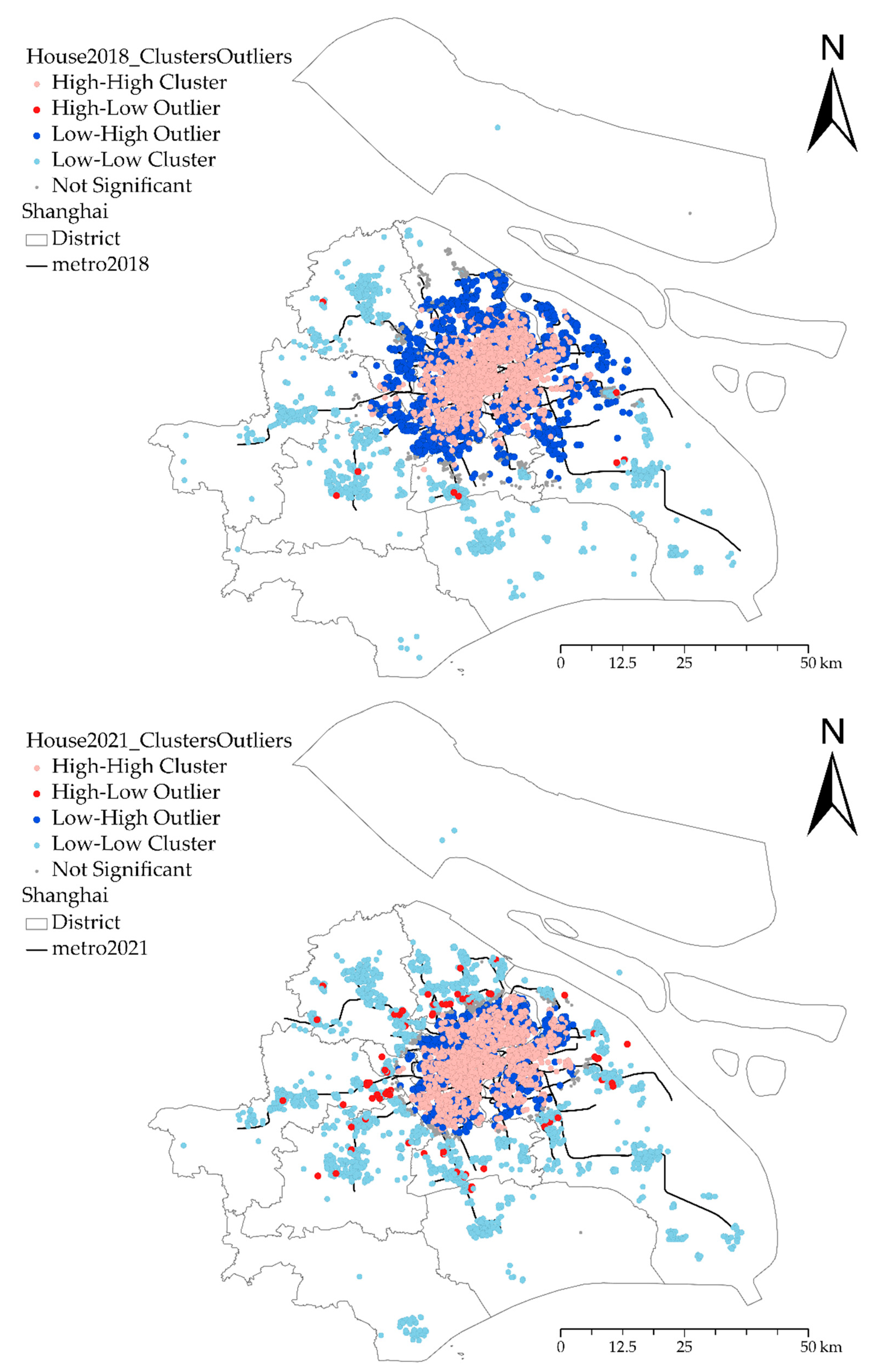
3.3. Hot Spot Analysis
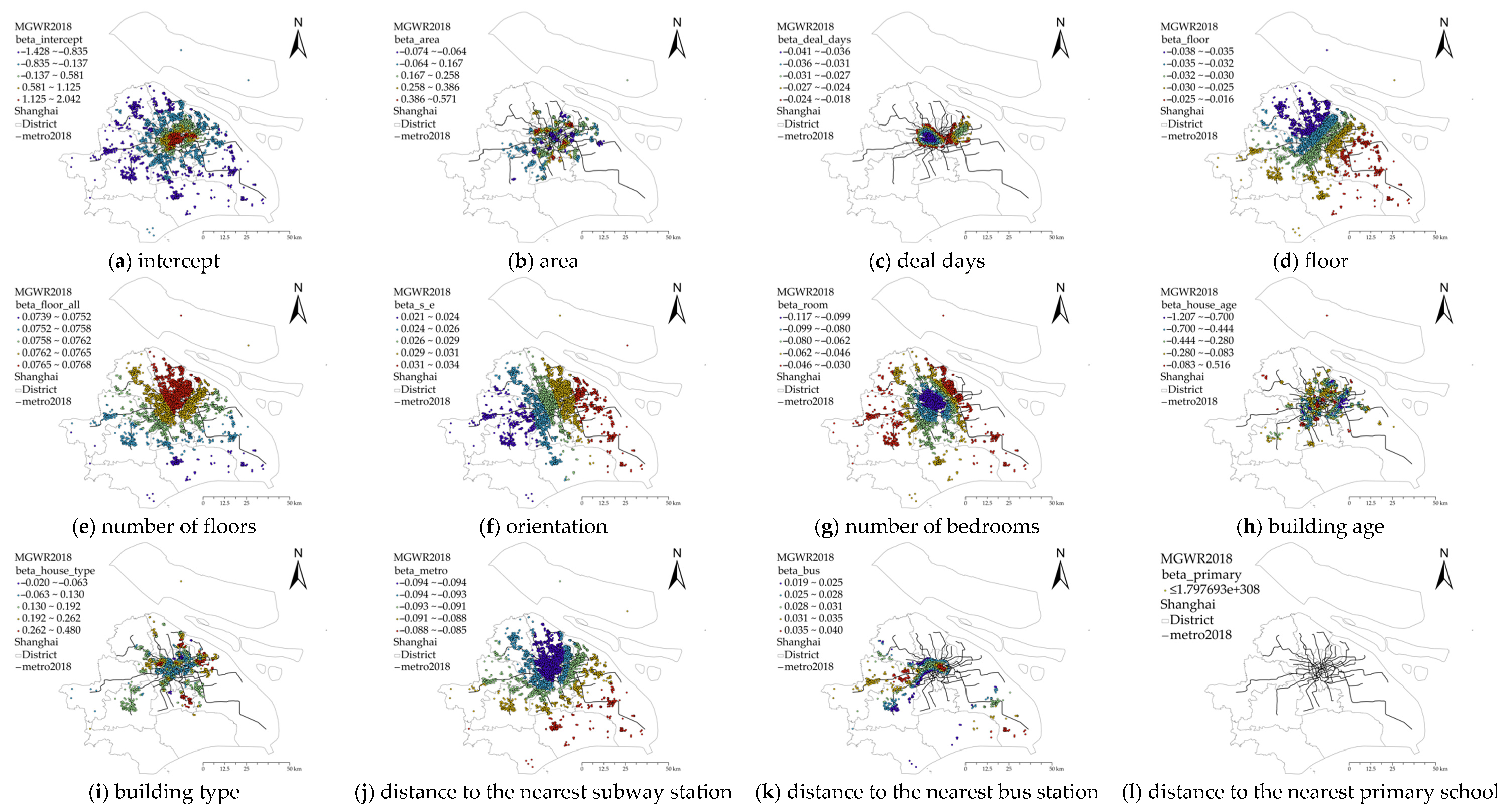
Results of a hot and cold spot analysis of Shanghai’s second-hand housing prices in 2018 and 2021 are shown in Figure 4. Almost all the area of Shanghai’s second-hand housing prices in 2018 were hot spots with 99% confidence, concentrated in a circular area about 50 km from downtown, whereas in 2021 the hot spots area sharply decreased to around only 20 km from the downtown city, the outside area being cold spots with 99% confidence.
Further examination is the cluster and outlier analysis of Shanghai’s second-hand housing prices in 2018 and 2021 (see Figure 5). In 2018, High-High (HH) Clusters were mainly concentrated inside the Middle Ring Road, all the Low-Low (LL) Clusters were distributed outside the Outer Ring Road, Low-High (LH) Outfitters were mixed between the HH Clusters and LL Clusters unevenly, while High-Low (HL) Outfitters were individually distributed in the suburbs of Shanghai. In 2021, spatial distribution patterns changed significantly compared to three years ago. HH Clusters’ range remained stable compared to 2018, with a slight expansion to the Minhang District. On the other hand, LL Clusters rose sharply, even invading inside the Outer Ring Road. Meanwhile, transition regions (LH Outfitters) were compressed significantly, with numbers of HL Outfitters rising greatly, distributed along the Outer Ring Road and subway line.
The newest changing patterns of Shanghai’s second-hand housing prices before and after the COVID-19 pandemic reveal that (1) the polarization of Shanghai’s housing price market has further intensified. (2) However, Shanghai’s housing prices have shown a trend of multi-centralization, and a considerable number of high-end properties have also appeared in suburban new towns. (3) Outside the central urban area, housing affordability in Shanghai has increased.

3.4. MGWR

Results of GWR and MGWR model indexes of Shanghai’s second-hand housing prices in 2018 and 2021 can be seen in Table 4. Seemingly, in both years, the residual sum of squares of MGWR is smaller than that of classical GWR, the goodness-of-fit R2 of MGWR is significantly higher than that of classical GWR, and the AICc value is lower than that of classical GWR. Therefore, it can be concluded that the result of MGWR is better than that of classical GWR. On the other hand, from the overall regression coefficient, almost all the coefficients of MGWR were significant—only significant results were drawn on the map, as shown in Figure 6 and Figure 7. In contrast, most coefficients of classical GWR are not statistically significant (not shown due to space constraints), which is unreasonable, and implies that the classical GWR ignores the diversification of the scale of each variable, resulting in a lot of noise and bias in the regression coefficients, and finally leads to inconsistencies in the regression coefficients. Therefore, based on the analysis results of this case, it is found that the MGWR model is superior to the classical GWR model, even under the shock of the pandemic.
It can be seen from Table 5 that MGWR can directly reflect the differential action scale of different variables. In contrast, the classical GWR can only reflect the average value of the action scale of each variable. The bandwidth of the classic GWR was 398 in 2018 and 285 in 2021, which was only 7.2% and 4.7% of the total sample size. By calculating MGWR, it was found that the scale of action of different variables varies greatly.
In 2018, the MGWR regression coefficients of 11 variables (namely constant term, area, transaction days, floor, number of floors, orientation, number of bedrooms, building age, building type, distance to the nearest subway station, and distance to the nearest bus station) were significant overall. However, the regression coefficient of distance to the nearest primary school was not significant. In 2021, the MGWR regression coefficients of 11 variables were also significant overall, except for the number of bedrooms.
The constant term represents the influence of different locations on house prices when other independent variables are determined. This paper controls traffic factors, so the constant term reflects the influence of other location factors such as school district and built environment on housing prices. The action scales were 44 in 2018 and 43 in 2021, accounting for 0.8% and 0.7% of the total sample size, which was much lower than the action scale of other variables, revealing that second-hand housing prices are very sensitive to the location in Shanghai.
In 2018, the role scale of the building age, living area, and building type were very small, accounting for less than 2.0% of the total sample size, indicating that those explanatory variables have large spatial heterogeneity. Action scales of the transaction days, number of bedrooms, and distance to the nearest bus station were relatively small, and the coefficient was relatively stable in space. However, effect scales of the floor, total floors, orientation, distance to the nearest subway station, and distance to the nearest primary school were pretty large, which belong to the global scale; that is, there was almost no spatial heterogeneity. Similarly, action scales of the explanatory variables in 2021 were also classified into 3 types: (1) very small: building age, living area, and total floors of the building; (2) relatively small: distance to the nearest primary school, building type, transaction days, orientation, distance to the nearest subway station, and floor of the house; (3) pretty large: number of bedrooms and distance to the nearest bus station.
The statistical description of each coefficient of MGWR is shown in Table 6. The impact of the location reflected by the constant term on the housing price was positive inside the Middle Ring Road and negative outside the Middle Ring Road in 2018, while positive inside the Inner Ring Road and negative outside the Inner Ring Road in 2021, showing an obvious circle structure in both years and an obvious shrinking range of expensive apartments after the pandemic, as can be seen in Figure 6a and Figure 7a.
As stated above, the action scale of different explanatory factors varies. In the MGWR model, a small variable coefficient means strong spatial heterogeneity; that is to say, the influence of this variable on housing prices varies greatly in communities with different geographical locations, which is shown as a relatively scattered distribution in the images, namely in Figure 6b,h,i and Figure 7b,d,h. On the contrary, a large variable coefficient means the variable has little effect on the housing price of different geographic locations and is shown through a regular color distribution in the images, namely, Figure 6d–f,j,l and Figure 7g,k.
The living area factor significantly impacts housing prices: negative inside the Inner Ring Road and outside the Outer Ring Road, while positive between those two roads in 2018 (see Figure 6b). The above phenomenon remained largely stable in 2021, with the Pudong district changing from negative to positive inside the Inner Ring Road area (see Figure 7b). Since Shanghai was developed from the central urban area, the average residential area is relatively small downtown, whereas land supply in suburban areas is relatively sufficient; thus, the average residential area is relatively large [2]. Negative effects inside the Inner Ring Road reflect that due to the large area, high unit price, and the high total price, the demand decreases, and then the unit price decreases. On the other hand, negative effects outside the Outer Ring Road demonstrate that location advantage disappears as the living area increases, and unit prices need to decrease to appeal to consumers. Moreover, positive impacts between the Inner Ring Road and outside the Outer Ring Road reveal that those areas are most suitable for dwellers to live and work, contributing to the rise of unit prices as the living area increases.
The transaction days have a significant negative impact, meaning that the higher the unit housing price, the shorter the transaction days. In 2018, transaction days’ impact was only significant inside the Outer Ring Road, and the absolute value of the coefficient was especially smaller along the Huangpu River. Nonetheless, the overall difference was small (see Figure 6c). In 2021, the absolute value of the coefficient rose sharply compared to that of 3 years ago (see Figure 7c). This shows obvious differences spatially, and older residential areas in the city have more serious price cuts.
The floor of the house is negatively connected to the housing price (see Figure 6d and Figure 7d). The floor factor is a dummy variable, where a bigger number means a higher floor, and less than 40% of houses are equipped with an elevator. It is reasonable that the higher the floor is, the lower the unit price is. Regarding spatial heterogeneity, negative impacts were deeper in the north-west region and lighter in the south-east area in 2018, whereas deeper in the south-west region and lighter in the south-east area in 2021. On the whole, negative affection was reinforced after the pandemic.
Overall, the number of floors of the building was positively connected with the housing price; the higher the building is, the higher the unit housing price is (see Figure 6e and Figure 7e). A taller building means a higher probability of owning an elevator, thus making the positive relationship between the house’s total floor and its housing price. In 2018, all the sample’s coefficients were positive and varied little; in 2021, the significant range shrunk greatly, and few residential area coefficients turned negative.
The house orientation also positively affects the unit price of the house. As China is located in the northern hemisphere, a house facing south or east enjoys better lighting and ventilation, which makes it more comfortable to live in. The better the house orientation (facing south or east), the higher the unit price, and the influence of this factor decreases from south-east to north-west, as shown in Figure 6f and Figure 7f. The house orientation coefficient’s mean value was 0.028 in 2018 and 0.059 in 2021, meaning houses facing west or north were RMB 28/59 lower than those facing east or south (see Table 6).
The number of bedrooms had a significant and negative impact on unit housing prices in 2018 but was not significant in 2021 (see Figure 6g and Figure 7g). In 2018, taking the downtown area as the core, the number of bedrooms had the greatest negative impact on the unit price, which spread outward in a circle with a gradually decaying effect. As mentioned above, housing prices in Shanghai are roughly distributed in a single-center pattern, with the highest housing prices in urban areas, which continue to decrease in circles. Therefore, high land prices in urban areas make the unit price of houses with fewer bedrooms and relatively smaller areas higher.
The influence of building age on the unit price was significantly negative in both years (see Figure 6h and Figure 7h). The building age coefficients’ mean value was −0.182 in 2018 and −0.204 in 2021, which means that for every 1-year increase in building age, the unit price of second-hand housing decreased RMB 182/204, reflecting that the negative impact of building age on housing prices is not different in different places, and its impact strength is weak (see Table 6).
Building type is also a dummy variable; most houses in Shanghai are a combination of slab-type and tower-type. Compared to the slab-type building, the unit house price of the combination type is higher globally. At the same time, spatial heterogeneity was not significant in 2018 and was notably high in the Pudong district inside the Inner Ring Road area in 2021 (see Figure 6i and Figure 7i).
The distance to the nearest subway station negatively affected the house price, while the distance to the nearest bus station positively affected the house price in both years. The farther the distance to the nearest bus station, the higher the housing price, which means that for Shanghai, where the transportation network covers a wider area, the negative externalities (such as crowding and noise) generated by the bus station have exceeded the positive externalities (such as transportation convenience), which is consistent with previous similar research [44,66]. Accordingly, the above results demonstrate that the metro serves as Shanghai’s most important transport vehicle [67]. In 2018, the distance to the nearest primary school showed no significant influence on the house price, while in 2021, the distance to the nearest primary school negatively affected the house price inside the Outer Ring Road while positively affecting the house price outside the Outer Ring Road, which reflects that families living near downtown care more about children’s education convenience (see Figure 6j–l and Figure 7j–l).

4. Conclusions

4.1. Summary of Results

This paper first applies the MGWR and hedonic price models with statistical inference at the forefront of academia to Shanghai’s empirical research. It distinguishes the newest changes under the shock of the COVID-19 pandemic. Combined with 283,075 pieces of second-hand housing transaction data from 2012 to 2021 in Shanghai, the spatial heterogeneity and spatial scale differences were studied. The following conclusions are drawn: first, compared with the classic GWR, the results of MGWR are more reliable. Previous studies based on classical GWR may have certain instability, but multi-MGWR can capture different influence scales of different variables and avoid capturing too much noise and bias. Therefore, whether the spatial scale of the influencing factors is considered will greatly impact the results and analysis of the model. Second, unit housing prices in Shanghai are centered on the city’s downtown, spreading radially to the surrounding areas, with suburbs’ houses distributed mainly along the subway branch line, and remaining stable as time passes. After the COVID-19 pandemic, the polarization of Shanghai’s housing price market intensified; housing prices in the downtown area rose higher, while prices in the outer suburbs declined. Third, housing prices are very sensitive to location and have strong spatial heterogeneity. The impact scale of location is the smallest among all variables, close to the street/township scale—the smallest grassroots mass autonomous organization in China. Other influences with spatial heterogeneity according to their spatial scale from small to large are as follows: building age, living area, building type, transaction days, bedrooms, and distance to the nearest bus stop in 2018; building age, living area, number of floors of the building, building type, distance to the nearest primary school, transaction days, orientation, distance to the nearest subway station, and floor of the house in 2021. The house floor, orientation, number of floors of the building, distance to the nearest subway station, and distance to the nearest primary school in 2018, as well as bedrooms, and distance to the nearest bus stop in 2021, were global-scale variables with weak spatial heterogeneity.

4.2. Policy Recommendations

4.2.1. Develop Multiple Urban Centers

Shanghai’s urban development model with the city center as a single center has reached an unsustainable level. The housing price far exceeds the income level of the working class. The salary income of ordinary employees who work for a whole year cannot afford a square meter inside Shanghai’s Inner Ring Road. Excessive housing prices are driving out innovative young people, thereby affecting the long-term development of cities [7,8,9]. Shanghai, the city with the largest population and the highest housing price in China, has realized this serious problem and has issued a multi-center urban plan of “Five New Cities” (“Shanghai Urban Master Plan (2017–2035)”) and the Pudong District’s emphasis on the Lingang area has also reached an unprecedented height (“14th Five-Year Plan for the Development of Lingang New Area of China (Shanghai) Pilot Free Trade Zone”). In the future, Shanghai’s urban development needs to further strengthen the construction of multiple urban sub-centers outside the downtown area, with industry as the guide, housing as the guarantee, and infrastructure as the support to promote more sustainable urban development.

4.2.2. Build Houses into Consumer’s Preferences in the Post-Epidemic Era

At the beginning of the COVID-19 epidemic, Shanghai, as a nationalized metropolis, took the lead in responding to various epidemic prevention policies and quickly brought the pandemic under control. Coupled with the difficult international and domestic situation, the real estate market in China’s super-first-tier cities became a relatively more secure investment channel, which has also led to a rapid increase in the transaction volume of second-hand housing in Shanghai in 2020 after the epidemic. However, in 2021, when the epidemic was relatively under control, the housing transaction volume dropped significantly again, and the housing elements that consumers cared about were more comprehensive. One of the most significant changes is the obvious increase in the living area. As of 2022, facing the sudden intensification of the epidemic situation in China, one of the measures adopted to prevent the epidemic is still closed management, where households are locked in their houses and are not allowed to go out. At present, the pandemic is still ongoing. In the face of unknown epidemic prevention policies in the future, consumers will inevitably have greater demands on the living area when purchasing a house. In the post-epidemic era, building homes outside the Inner Ring Road, which have bigger living areas, higher total floors (elevator-equipped), and are closer to subway stations (which is the most common mode of transportation for Shanghai residents to travel and go to work), will be more in line with market needs.

4.2.3. Improve Infrastructure Construction

Before and after the epidemic, the “distance to the nearest subway station” indicator significantly negatively impacted house prices and demonstrated a clear circle structure. As the economic center of the world’s largest developing country and one of the international financial hubs, Shanghai’s economic development is inseparable from the hard work of thousands of residents. The Shanghai government has built a city-wide industrial map (https://map.sheitc.sh.gov.cn/#/index (accessed on 21 July)) based on the respective endowments of the 16 administrative regions, striving to achieve differentiated and comprehensive development. However, the role of industrial agglomeration in promoting economic growth will inevitably lead to the decentralized concentration of jobs all over the city, which will impact residents’ commuting. Therefore, further improving the infrastructure construction of the whole city and building a relatively economical way of travel—mainly the subway—is still an important measure for the city’s sustainable development.

4.3. Limitations of the Study

In this study, we could only focus on Shanghai when exploring the spatial heterogeneity and main influencing factors pre- and post- COVID-19 in megacities. Although Shanghai is one of the most important cities in China and the world, its experiences can only give limited suggestions to other megacities worldwide. Specific practices should be carried out according to local economic and political situations. The MGWR model also has its limitations; in this study, the total number of observations was 5548 in 2018 and 6042 in 2021, and each year takes more than 10 h to run the model on the software MGWR (https://sgsup.asu.edu/sparc/multiscale-gwr (accessed on 5 July)). To our knowledge, this paper has the largest sample size using the MGWR model. Future research using this method might face software limitations if the sample size is too large. Additionally, we chose traditional influencing factors, which may not be comprehensive enough to explain housing prices; future researchers could explore more innovative variables.

Author Contributions

Conceptualization, Y.C.; Funding acquisition, Z.L.; Resources, Z.L.; Software, Y.C.; Supervision, Z.L.; Writing—original draft, Y.C.; Writing—review & editing, Y.C. All authors have read and agreed to the published version of the manuscript.

Funding

This research received no external funding.

Institutional Review Board Statement

Not applicable.

Conflicts of Interest

The authors declare no conflict of interest.

References

  1. He, C.; Wang, Z.; Guo, H.; Sheng, H.; Zhou, R.; Yang, Y. Driving Forces Analysis for Residential Housing Price in Beijing. Procedia Environ. Sci. 2010, 2, 925–936. [Google Scholar] [CrossRef]
  2. Huang, Z.; Chen, R.; Xu, D.; Zhou, W. Spatial and Hedonic Analysis of Housing Prices in Shanghai. Habitat Int. 2017, 67, 69–78. [Google Scholar] [CrossRef]
  3. Hui, E.C.M.; Yue, S. Housing Price Bubbles in Hong Kong, Beijing and Shanghai: A Comparative Study. J. Real Estate Financ. Econ. 2006, 33, 299–327. [Google Scholar] [CrossRef]
  4. Li, N.; Li, R.Y.M.; Pu, R. What Is in a Name? A Modern Interpretation from Housing Price in Hong Kong. Pac. Rim Prop. Res. J. 2021, 27, 55–74. [Google Scholar] [CrossRef]
  5. Piao, Y.; Chen, A.; Shang, Z. Housing Price Prediction Based on CNN. In Proceedings of the 2019 9th International Conference on Information Science and Technology (ICIST), Cairo, Egypt, 24–26 March 2019; IEEE: Hulunbuir, China, 2019; pp. 491–495. [Google Scholar]
  6. Shanghai Bureau of Statistics. A Review of Shanghai Real Estate Market in 2021. Available online: http://tjj.sh.gov.cn/tjfx/20220129/f49f612d4ec548adbe5db5c91466b324.html (accessed on 29 January 2022).
  7. Chan, S. Spatial Lock-in: Do Falling House Prices Constrain Residential Mobility? J. Urban Econ. 2001, 49, 567–586. [Google Scholar] [CrossRef]
  8. Shan, H. Property Taxes and Elderly Mobility. J. Urban Econ. 2010, 67, 194–205. [Google Scholar] [CrossRef]
  9. Yang, Z.; Pan, Y. Human Capital, Housing Prices, and Regional Economic Development: Will “Vying for Talent” through Policy Succeed? Cities 2020, 98, 102577. [Google Scholar] [CrossRef]
  10. Can, A. Specification and Estimation of Hedonic Housing Price Models. Reg. Sci. Urban Econ. 1992, 22, 453–474. [Google Scholar] [CrossRef]
  11. Court, L.M. Entrepreneurial and Consumer Demand Theories for Commodity Spectra: Part I. Econometrica 1941, 9, 135. [Google Scholar] [CrossRef]
  12. Freeman, A.M. The Hedonic Price Approach to Measuring Demand for Neighborhood Characteristics. In The Economics of Neighborhood; Elsevier: Amsterdam, The Netherlands, 1979; pp. 191–217. ISBN 978-0-12-636250-3. [Google Scholar]
  13. Rosen, S. Hedonic Prices and Implicit Markets: Product Differentiation in Pure Competition. J. Political Econ. 1974, 82, 34–55. [Google Scholar] [CrossRef]
  14. Tinbergen, J. On the Theory of Income Distribution. Weltwirtschaftliches Arch. 1956, 77, 155–175. [Google Scholar]
  15. Li, R.; Cheung, K.; Shoaib, M. Walled Buildings, Sustainability, and Housing Prices: An Artificial Neural Network Approach. Sustainability 2018, 10, 1298. [Google Scholar] [CrossRef]
  16. Wang, R.; Hou, J. Land Finance, Land Attracting Investment and Housing Price Fluctuations in China. Int. Rev. Econ. Financ. 2021, 72, 690–699. [Google Scholar] [CrossRef]
  17. Harrison, D.; Rubinfeld, D.L. Hedonic Housing Prices and the Demand for Clean Air. J. Environ. Econ. Manag. 1978, 5, 81–102. [Google Scholar] [CrossRef]
  18. Michaels, R.G.; Smith, V.K. Market Segmentation and Valuing Amenities with Hedonic Models: The Case of Hazardous Waste Sites. J. Urban Econ. 1990, 28, 223–242. [Google Scholar] [CrossRef]
  19. Straszheim, M.R. Hedonic Estimation of Housing Market Prices: A Further Comment. Rev. Econ. Stat. 1974, 56, 404–406. [Google Scholar] [CrossRef]
  20. Kain, J.F.; Quigley, J.M. Measuring the Value of Housing Quality. J. Am. Stat. Assoc. 1970, 65, 532–548. [Google Scholar] [CrossRef]
  21. Sirmans, G.S.; MacDonald, L.; Macpherson, D.A.; Zietz, E.N. The Value of Housing Characteristics: A Meta Analysis. J. Real Estate Financ. Econ. 2006, 33, 215–240. [Google Scholar] [CrossRef]
  22. Heikkila, E.; Gordon, P.; Kim, J.I.; Peiser, R.B.; Richardson, H.W.; Dale-Johnson, D. What Happened to the CBD-Distance Gradient?: Land Values in a Policentric City. Environ. Plan. A 1989, 21, 221–232. [Google Scholar] [CrossRef]
  23. Osland, L.; Thorsen, I. Effects on Housing Prices of Urban Attraction and Labor-Market Accessibility. Environ. Plan. A 2008, 40, 2490–2509. [Google Scholar] [CrossRef]
  24. Richardson, H.W.; Gordon, P.; Jun, M.-J.; Heikkila, E.; Peiser, R.; Dale-Johnson, D. Residential Property Values, the CBD, and Multiple Nodes: Further Analysis. Environ. Plan. A 1990, 22, 829–833. [Google Scholar] [CrossRef]
  25. Dubin, R.A.; Goodman, A.C. Valuation of Education and Crime Neighborhood Characteristics through Hedonic Housing Prices. Popul. Environ. 1982, 5, 166–181. [Google Scholar] [CrossRef]
  26. Gibbons, S.; Machin, S. Valuing English Primary Schools. J. Urban Econ. 2003, 53, 197–219. [Google Scholar] [CrossRef]
  27. Brasington, D.M.; Hite, D. Demand for Environmental Quality: A Spatial Hedonic Analysis. Reg. Sci. Urban Econ. 2005, 35, 57–82. [Google Scholar] [CrossRef]
  28. Das, R.C.; Chatterjee, T.; Ivaldi, E. Nexus between Housing Price and Magnitude of Pollution: Evidence from the Panel of Some High- and-Low Polluting Cities of the World. Sustainability 2022, 14, 9283. [Google Scholar] [CrossRef]
  29. Poudyal, N.C.; Hodges, D.G.; Merrett, C.D. A Hedonic Analysis of the Demand for and Benefits of Urban Recreation Parks. Land Use Policy 2009, 26, 975–983. [Google Scholar] [CrossRef]
  30. Fletcher, M.; Gallimore, P.; Mangan, J. Heteroscedasticity in Hedonic House Price Models. J. Prop. Res. 2000, 17, 93–108. [Google Scholar] [CrossRef]
  31. Goodman, A.C. Hedonic Prices, Price Indices and Housing Markets. J. Urban Econ. 1978, 5, 471–484. [Google Scholar] [CrossRef]
  32. Goodman, A.C.; Thibodeau, T.G. Dwelling-Age-Related Heteroskedasticity in Hedonic House Price Equations: An Extension. J. Hous. Res. 1997, 8, 299–317. [Google Scholar]
  33. Miller, H.J. Tobler’s First Law and Spatial Analysis. Ann. Assoc. Am. Geogr. 2004, 94, 284–289. [Google Scholar] [CrossRef]
  34. Wong, W.S.D.; Lee, J. Statistical Analysis of Geographic Information with ArcView GIS and ArcGIS; Wiley: Hoboken, NJ, USA, 2005; ISBN 0-471-46899-1. [Google Scholar]
  35. Cleveland, W.S.; Devlin, S.J. Locally Weighted Regression: An Approach to Regression Analysis by Local Fitting. J. Am. Stat. Assoc. 1988, 83, 596–610. [Google Scholar] [CrossRef]
  36. Wang, C.; Du, S.; Wen, J.; Zhang, M.; Gu, H.; Shi, Y.; Xu, H. Analyzing Explanatory Factors of Urban Pluvial Floods in Shanghai Using Geographically Weighted Regression. Stoch Env. Res Risk Assess 2017, 31, 1777–1790. [Google Scholar] [CrossRef]
  37. Wheeler, D.C.; Páez, A. Geographically Weighted Regression. In Handbook of Applied Spatial Analysis; Springer: Berlin/Heidelberg, Germany, 2010; pp. 461–486. [Google Scholar]
  38. Cho, S.; Lambert, D.M.; Kim, S.G.; Jung, S. Extreme Coefficients in Geographically Weighted Regression and Their Effects on Mapping. GIScience Remote Sens. 2009, 46, 273–288. [Google Scholar] [CrossRef]
  39. Wheeler, D.; Tiefelsdorf, M. Multicollinearity and Correlation among Local Regression Coefficients in Geographically Weighted Regression. J Geogr. Syst 2005, 7, 161–187. [Google Scholar] [CrossRef]
  40. Fotheringham, A.S.; Brunsdon, C.; Charlton, M. Geographically Weighted Regression: The Analysis of Spatially Varying Relationships; John Wiley & Sons: Hoboken, NJ, USA, 2003; ISBN 0-470-85525-8. [Google Scholar]
  41. Fotheringham, A.S.; Yang, W.; Kang, W. Multiscale Geographically Weighted Regression (MGWR). Ann. Am. Assoc. Geogr. 2017, 107, 1247–1265. [Google Scholar] [CrossRef]
  42. Oshan, T.M.; Smith, J.P.; Fotheringham, A.S. Targeting the Spatial Context of Obesity Determinants via Multiscale Geographically Weighted Regression. Int. J. Health Geogr. 2020, 19, 11. [Google Scholar] [CrossRef]
  43. Gao, L.; Huang, M.; Zhang, W.; Qiao, L.; Wang, G.; Zhang, X. Comparative Study on Spatial Digital Mapping Methods of Soil Nutrients Based on Different Geospatial Technologies. Sustainability 2021, 13, 3270. [Google Scholar] [CrossRef]
  44. Shen, T.Y.; Yu, H.C.; Zhou, L.; Gu, H.; He, H. On Hedonic Price of Second-Hand Houses in Beijing Based on Multi-Scale Geographically Weighted Regression: Scale Law of Spatial Heterogeneity. Econ. Geogr. 2020, 40, 75–83. [Google Scholar] [CrossRef]
  45. Li, S.; Ye, X.; Lee, J.; Gong, J.; Qin, C. Spatiotemporal Analysis of Housing Prices in China: A Big Data Perspective. Appl. Spat. Anal. 2017, 10, 421–433. [Google Scholar] [CrossRef]
  46. Zheng, S.; Kahn, M.E.; Liu, H. Towards a System of Open Cities in China: Home Prices, FDI Flows and Air Quality in 35 Major Cities. Reg. Sci. Urban Econ. 2010, 40, 1–10. [Google Scholar] [CrossRef]
  47. Hou, Y. Housing Price Bubbles in Beijing and Shanghai?: A Multi-indicator Analysis. Int. J. Hous. Mark. Anal. 2010, 3, 17–37. [Google Scholar] [CrossRef]
  48. Li, L.H.; Ge, C.L. Inflation and Housing Market in Shanghai. Prop. Manag. 2008, 26, 273–288. [Google Scholar]
  49. Liu, C.; Lu, J.; Fu, W.; Zhou, Z. Second-Hand Housing Batch Evaluation Model of Zhengzhou City Based on Big Data and MGWR Model. IFS 2022, 42, 4221–4240. [Google Scholar] [CrossRef]
  50. Wen, H.; Jin, Y.; Zhang, L. Spatial Heterogeneity in Implicit Housing Prices: Evidence from Hangzhou, China. Int. J. Strateg. Prop. Manag. 2017, 21, 15–28. [Google Scholar] [CrossRef]
  51. Liu, L.; Yu, H.; Zhao, J.; Wu, H.; Peng, Z.; Wang, R. Multiscale Effects of Multimodal Public Facilities Accessibility on Housing Prices Based on MGWR: A Case Study of Wuhan, China. IJGI 2022, 11, 57. [Google Scholar] [CrossRef]
  52. Jones, L.; Palumbo, D.; Brown, D. Coronavirus: How the Pandemic Has Changed the World Economy. BBC News 2021. [Google Scholar]
  53. Pak, A.; Adegboye, O.A.; Adekunle, A.I.; Rahman, K.M.; McBryde, E.S.; Eisen, D.P. Economic Consequences of the COVID-19 Outbreak: The Need for Epidemic Preparedness. Front. Public Health 2020, 8, 241. [Google Scholar] [CrossRef]
  54. Del Giudice, V.; De Paola, P.; Del Giudice, F.P. COVID-19 Infects Real Estate Markets: Short and Mid-Run Effects on Housing Prices in Campania Region (Italy). Soc. Sci. 2020, 9, 114. [Google Scholar] [CrossRef]
  55. Li, X.; Zhang, C. Did the COVID-19 Pandemic Crisis Affect Housing Prices Evenly in the U.S.? Sustainability 2021, 13, 12277. [Google Scholar] [CrossRef]
  56. Qian, X.; Qiu, S.; Zhang, G. The Impact of COVID-19 on Housing Price: Evidence from China. Financ. Res. Lett. 2021, 43, 101944. [Google Scholar] [CrossRef]
  57. Tanrıvermiş, H. Possible Impacts of COVID-19 Outbreak on Real Estate Sector and Possible Changes to Adopt: A Situation Analysis and General Assessment on Turkish Perspective. J. Urban Manag. 2020, 9, 263–269. [Google Scholar] [CrossRef]
  58. Zhang, H. Cultural Diversity, Cooperation Spirit and Team Efficiency. Bus. Manag. J. 2022, 44, 108–122. [Google Scholar] [CrossRef]
  59. Li, H.; Wei, Y.D.; Wu, Y.; Tian, G. Analyzing Housing Prices in Shanghai with Open Data: Amenity, Accessibility and Urban Structure. Cities 2019, 91, 165–179. [Google Scholar] [CrossRef]
  60. Li, H.; Chen, P.; Grant, R. Built Environment, Special Economic Zone, and Housing Prices in Shenzhen, China. Appl. Geogr. 2021, 129, 102429. [Google Scholar] [CrossRef]
  61. Yu, H.; Hou, Y. A Tale of Two Districts: The Impact of District Consolidation on Property Values in Shanghai. Reg. Sci. Urban Econ. 2021, 87, 103647. [Google Scholar] [CrossRef]
  62. Tobler, W.R. A Computer Movie Simulating Urban Growth in the Detroit Region. Econ. Geogr. 1970, 46, 234. [Google Scholar] [CrossRef]
  63. Moran, P.A.P. Notes on Continuous Stochastic Phenomena. Biometrika 1950, 37, 17. [Google Scholar] [CrossRef]
  64. Ord, J.K.; Getis, A. Local Spatial Autocorrelation Statistics: Distributional Issues and an Application. Geogr. Anal. 1995, 27, 286–306. [Google Scholar] [CrossRef]
  65. Hui, D.S.; I Azhar, E.; Madani, T.A.; Ntoumi, F.; Kock, R.; Dar, O.; Ippolito, G.; Mchugh, T.D.; Memish, Z.A.; Drosten, C.; et al. The Continuing 2019-NCoV Epidemic Threat of Novel Coronaviruses to Global Health—The Latest 2019 Novel Coronavirus Outbreak in Wuhan, China. Int. J. Infect. Dis. 2020, 91, 264–266. [Google Scholar] [CrossRef]
  66. Cui, N.; Gu, H.; Shen, T.; Zhou, L.; Cui, D. Research on the Influence of Traffic Spatial Layout on Urban Housing Price—Based on the Analysis of the Correlation between Beijing Road Network Configuration and Housing Price. Price Theory Pract. 2019, 2, 63–66. [Google Scholar] [CrossRef]
  67. Wang, Y. Study on the Temporal and Spatial Characteristics of Shanghai Residents’ Travel Based on Public Transport Big Data; Shandong Normal University: Jinan, China, 2018. [Google Scholar]
Figure 1. Map of Shanghai. Source: drawn by authors, based on Shanghai Standard Map from Shanghai Surveying and Mapping Institute (https://www.shsmi.cn/wcm.files/upload/CMSCHY/202112/202112070757044.jpg).
Sustainability 14 11021 g001
Figure 2. Boxplot of Shanghai house prices (2012–2021). Source: drawn by authors, based on Lianjia Real Estate’s data.
Sustainability 14 11021 g002
Figure 3. Shanghai second-hand house prices (2018, 2021). Source: drawn by authors.
Sustainability 14 11021 g003
Figure 4. Cold and hot spots of second-hand house prices in Shanghai (2018, 2021). Source: drawn by authors.
Sustainability 14 11021 g004
Figure 5. Clusters-Outliers of second-hand house prices in Shanghai (2018, 2021). Source: drawn by authors.
Sustainability 14 11021 g005
Figure 6. Spatial patterns of coefficients in the MGWR (2018). Source: drawn by authors.
Sustainability 14 11021 g006
Figure 7. Spatial patterns of coefficients in the MGWR (2021). Source: drawn by authors.
Sustainability 14 11021 g007
Table 1. Description of major variables (authors’ results).
Variable TypesVariableUnitDescription
Dependent variablepriceRMB 10,000/m2Shanghai’s second-hand housing prices
Structural attributesareaSquare meterResidential(living) area of the house
deal_daysDaysTransaction time of the house
floorDiscrete variableFloor of the house (villa with basement: 1; low floor: 2; middle floor: 3; high floor: 4)
floor_allFloorNumber of floors of the building (1–56)
s_eVirtual variableOrientation of the house (whether the house faces south or east, Yes: 1; No: 0)
roomRoomNumber of residential bedrooms (1–9)
house_ageYearAge of the building (years between deal year and construction year, 0–109)
house_typeDiscrete variableBuilding type of the building (slab-type apartment building: 1; bungalow: 2; tower-type apartment building: 3; combination: 4)
Locational attributesmetroMeterDistance to the nearest subway station
busMeterDistance to the nearest bus stop
primaryMeterDistance to the nearest elementary school
interceptRMB 10,000The intercept term of the model, reflecting the effect of location
Table 2. Characteristics of second-hand houses in Shanghai (2018, 2021) (authors’ results).
VariablePercentage/Mean Value
20182021
price5.196.27
area74.7087.63
deal_days144.0292.55
floor3.053.05
1: villa with basement0.030.08
2: low floor29.6332.05
3: middle floor35.7530.42
4: high floor34.6237.46
floor_all10.2110.70
s_e
03.254.24
196.7595.76
room1.801.82
house_age20.1023.13
house_type
1: slab-type9.3210.63
2: bungalow0.110.12
3: tower-type0.401.07
4: combination90.1788.18
metro1210.881182.90
bus176.43166.66
primary543.89549.68
Table 3. Results of auto-correlation analysis (authors’ results).
Variable20182021
Moran’s Index0.5790.603
Expected Index−0.005−0.005
Variance0.0000.000
z-score34.04334.019
p-value0.0000.000
Table 4. Model index of GWR and MGWR (2018, 2021) (authors’ results).
Index20182021
GWRMGWRGWRMGWR
Residual sum of squares3808.84800.964352.27876.55
Log-likelihood:−6828.94−2503.53−7582.22−2741.19
AICc:13,683.947079.4715,190.507932.55
Adj. R20.3120.8290.2780.826
Table 5. Bandwidth of GWR and MGWR (2018, 2021) (authors’ results).
Variable20182021
GWRMGWRGWRMGWR
intercept3984428543
area3987728584
deal_days3981756285508
floor39848722852176
floor_all3985546285110
s_e3985049285601
room39819562856041
house_age3984628544
house_type398111285484
metro39855462851005
bus39819572856041
primary3985546285478
Table 6. Statistical description of MGWR coefficient (authors’ results).
MeanSTDMinMedianMax
Year 2018
intercept−0.0010.849−1.428−0.0092.042
area0.0670.163−0.7380.0650.571
deal_days−0.0140.015−0.041−0.0140.014
floor−0.0310.004−0.038−0.032−0.016
floor_all0.0760.0000.0740.0760.077
s_e0.0280.0030.0210.0280.034
room−0.0690.028−0.117−0.068−0.018
house_age−0.1820.227−1.207−0.1460.516
house_type0.1040.099−0.3110.1040.480
metro−0.0930.002−0.095−0.093−0.085
bus0.0170.011−0.0090.0190.040
primary−0.0090.001−0.012−0.009−0.007
Year 2021
intercept−0.1660.733−1.847−0.1241.729
area0.0390.166−0.4100.0310.579
deal_days−0.0990.041−0.218−0.1000.014
floor−0.0350.013−0.065−0.0370.000
floor_all0.0780.094−0.1800.0720.399
s_e0.0590.041−0.0630.0560.175
room−0.0040.000−0.005−0.005−0.002
house_age−0.2040.239−1.286−0.1660.735
house_type0.1340.051−0.0120.1370.287
metro−0.7880.330−1.266−0.911−0.103
bus0.0160.0000.0150.0160.017
primary−0.0450.076−0.287−0.0290.174
Publisher’s Note: MDPI stays neutral with regard to jurisdictional claims in published maps and institutional affiliations.

