Experimental Validation of a High Precision GNSS System for Monitoring of Civil Infrastructures
Abstract
:1. Introduction
2. Materials and Methods
2.1. Benchmark Structure and Test Configuration
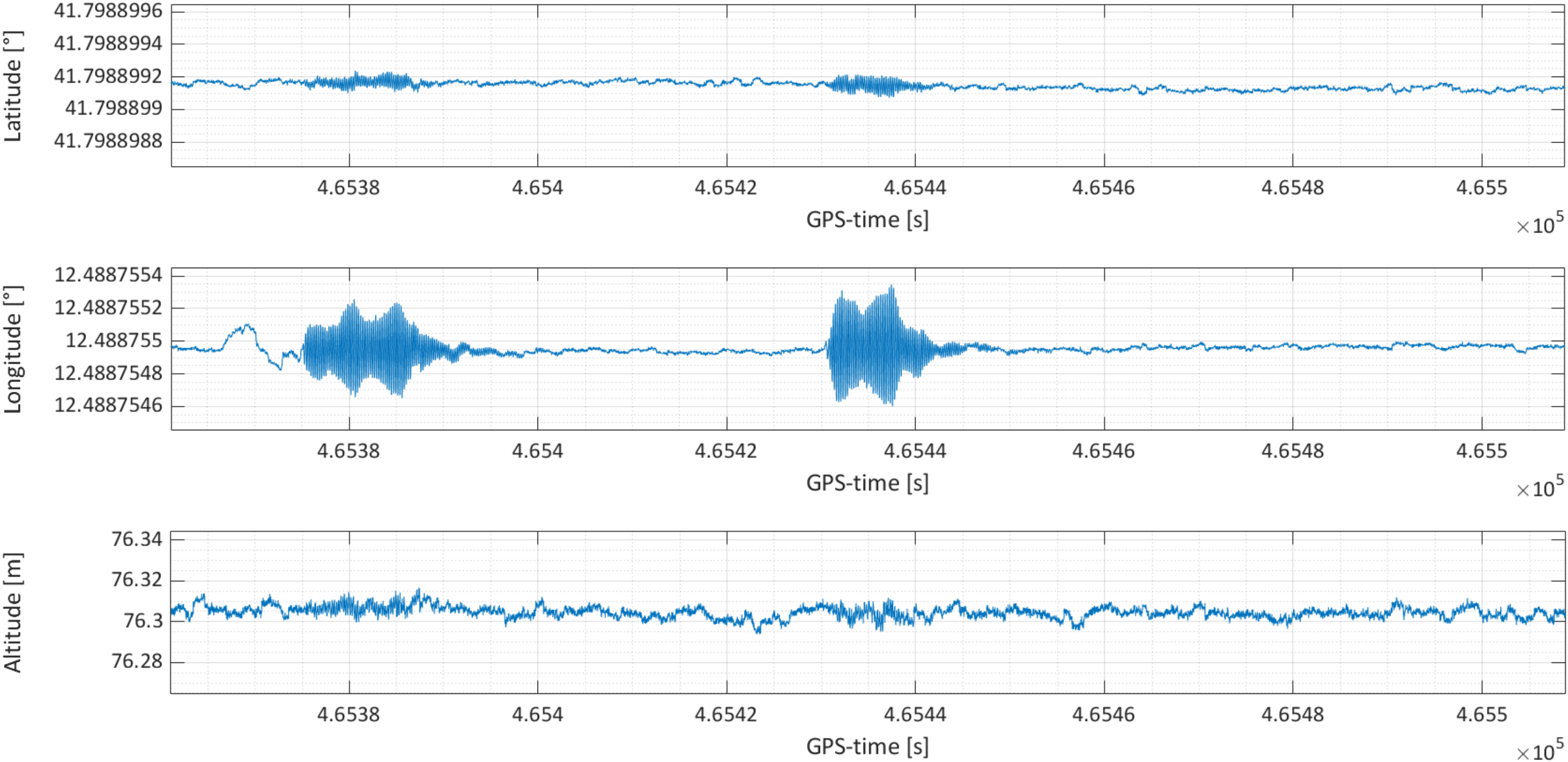
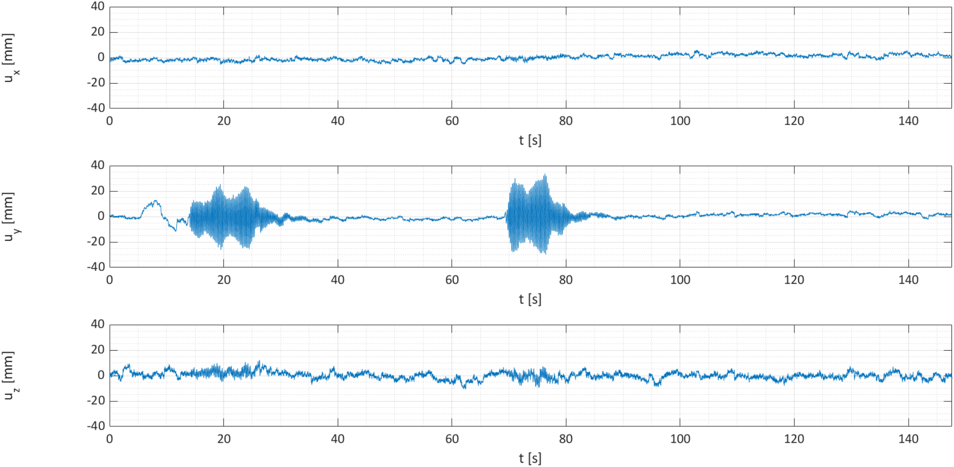
2.2. Analysis of the GNSS Signal
2.3. Validation
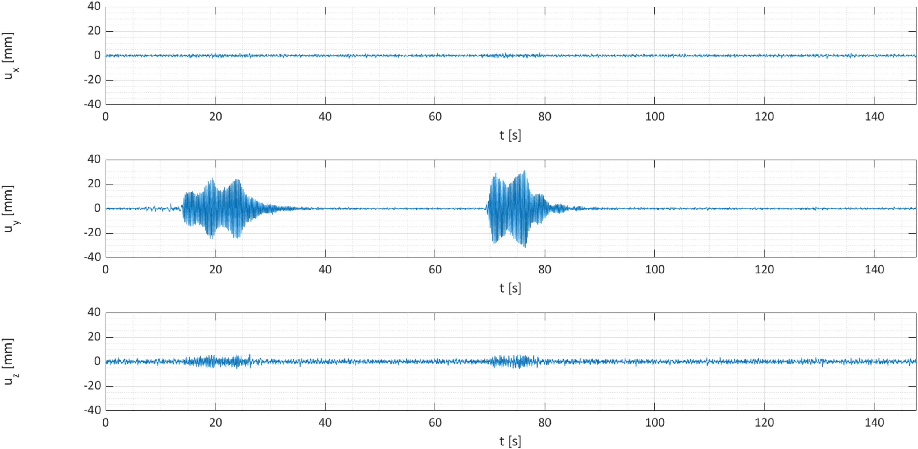
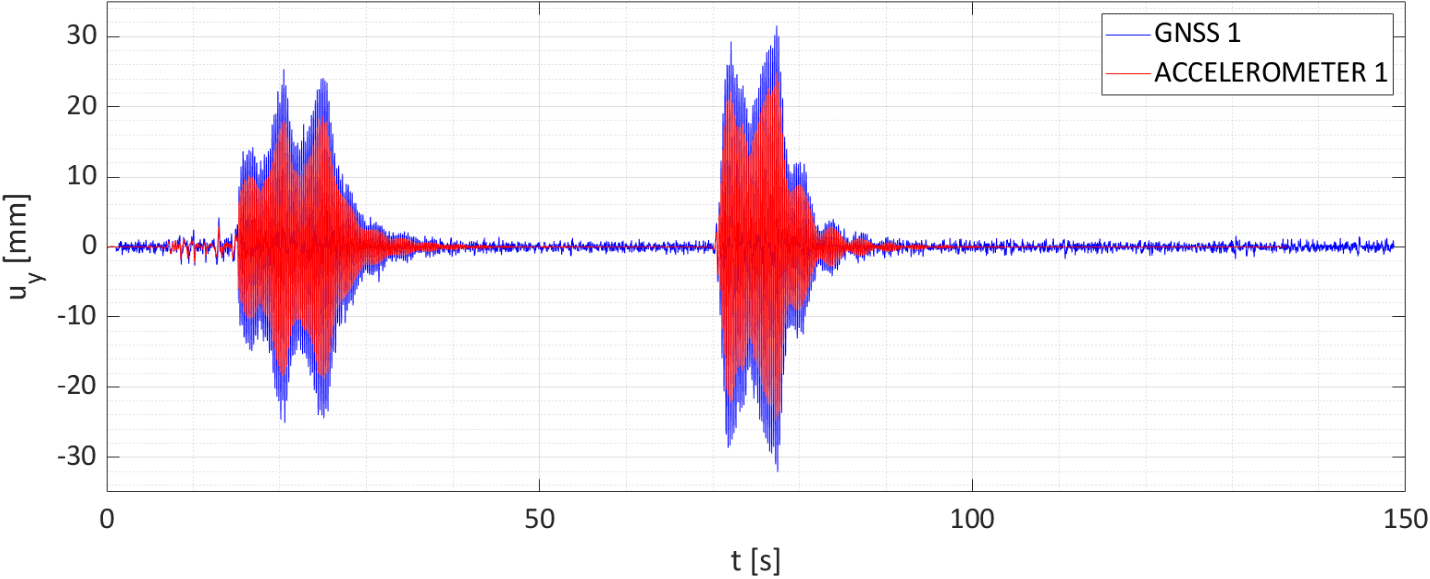
2.3.1. Time Domain
2.3.2. Frequency Domain
3. Results on a Real Bridge
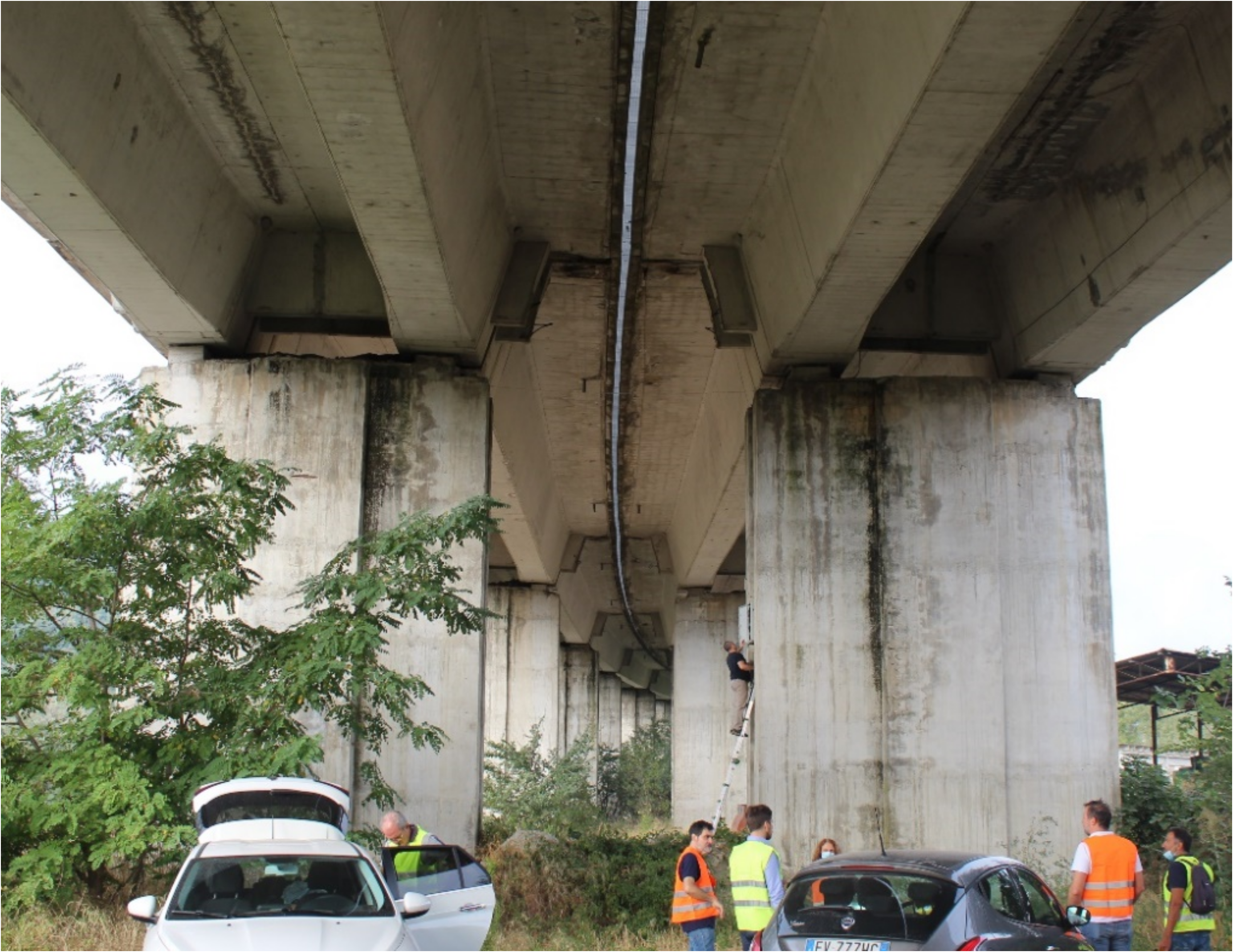
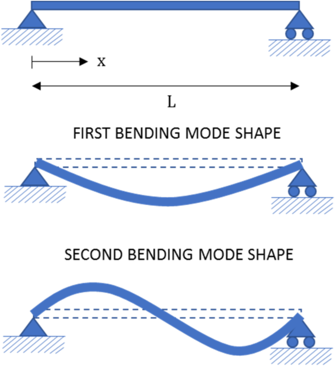
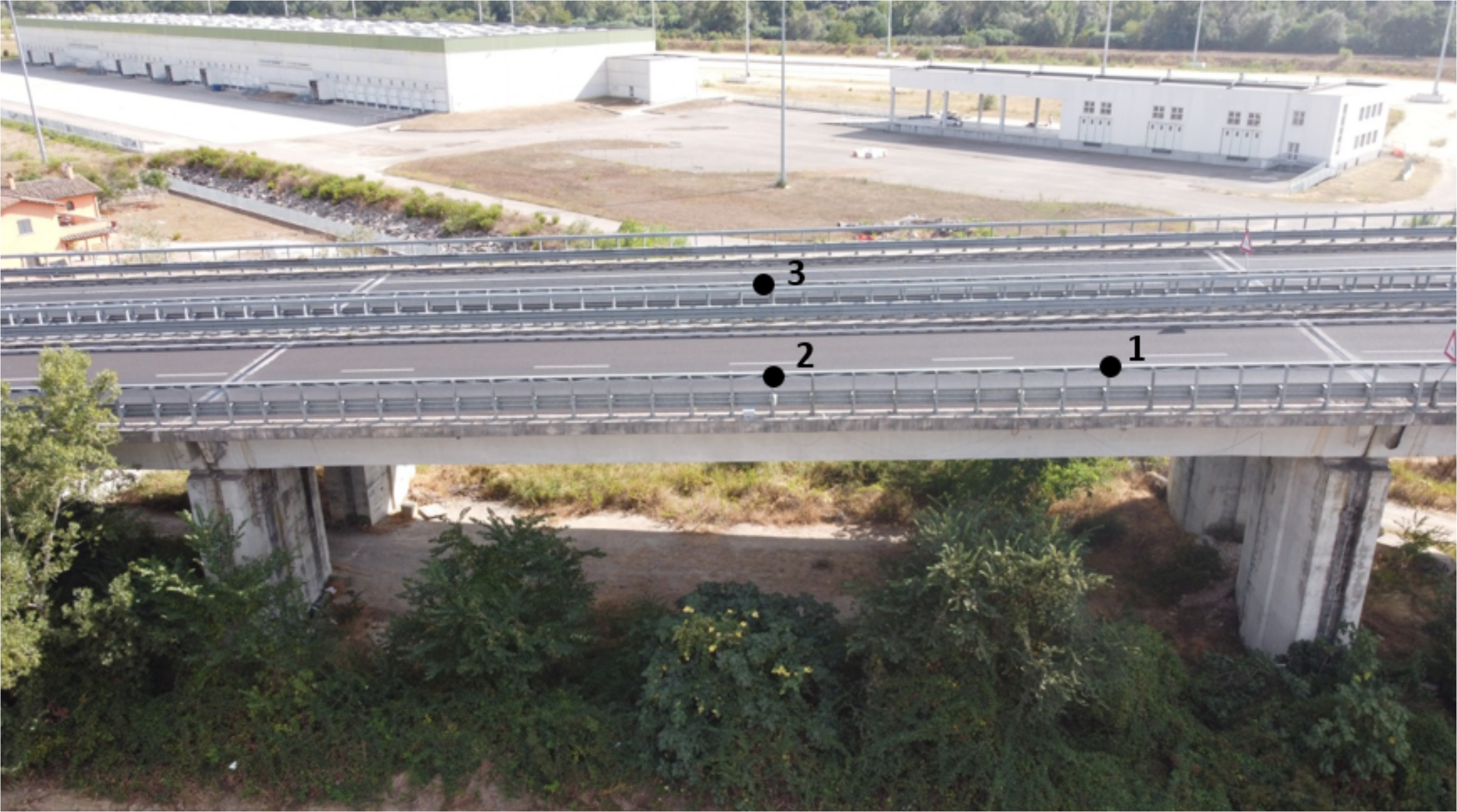
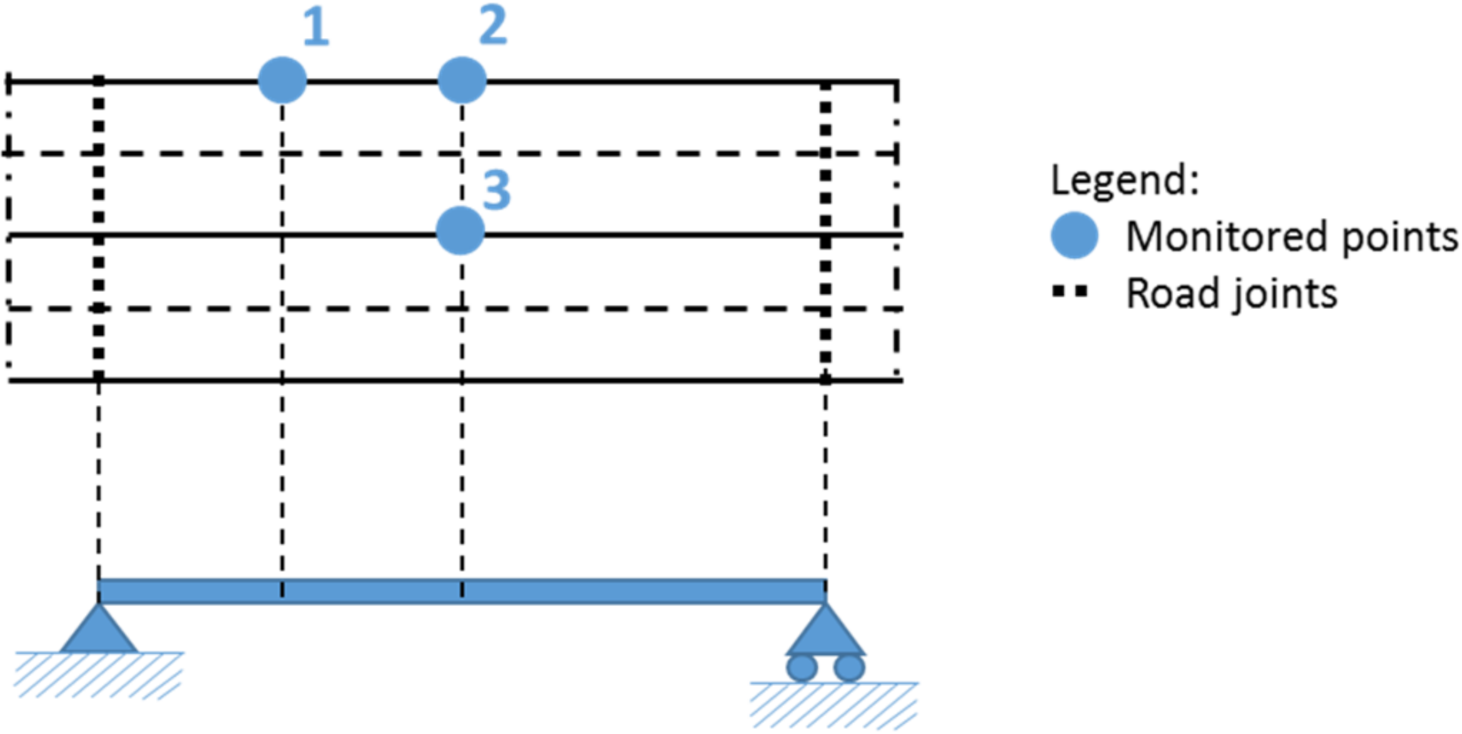
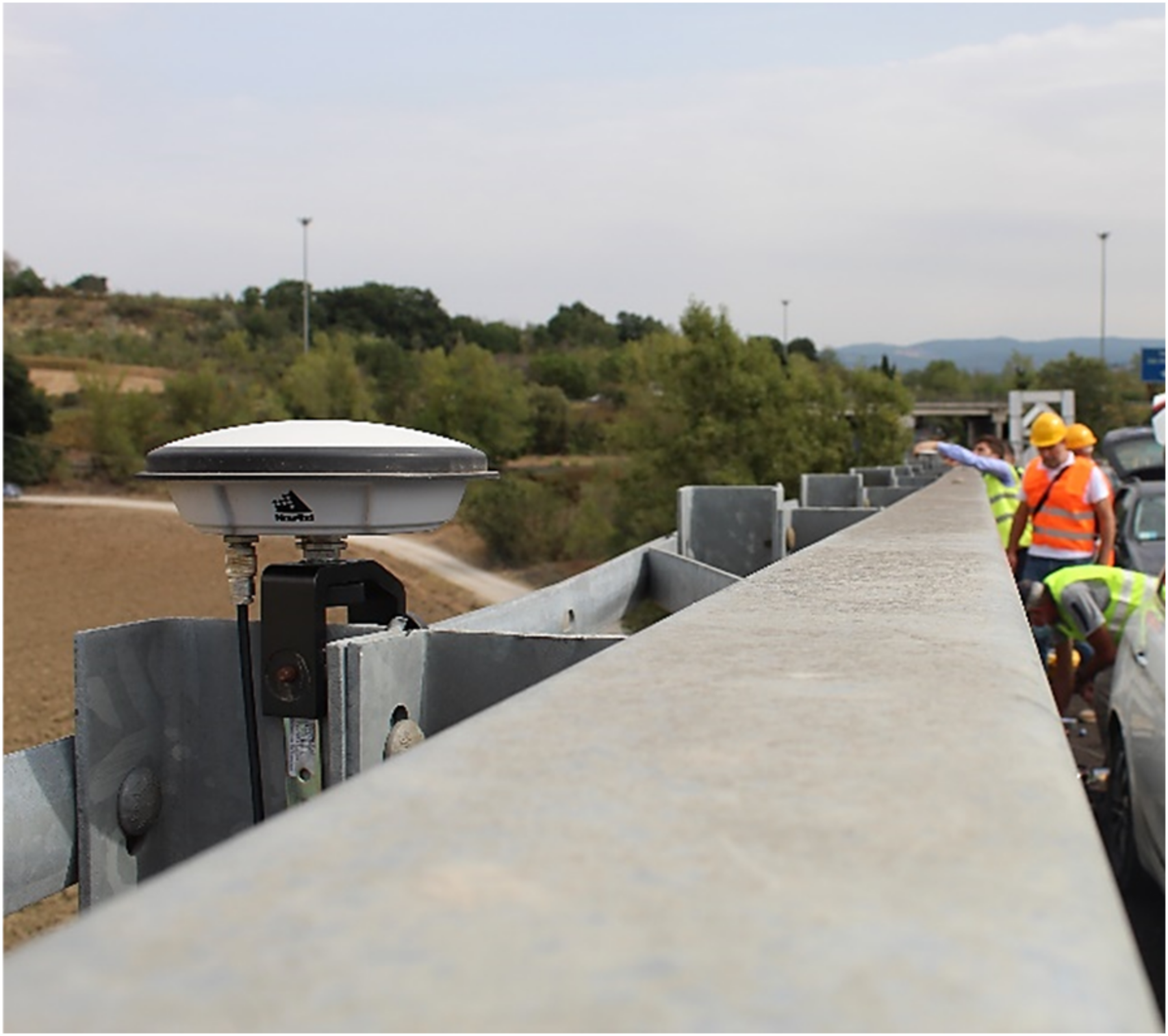
3.1. Benchmark Structure and Test Configuration
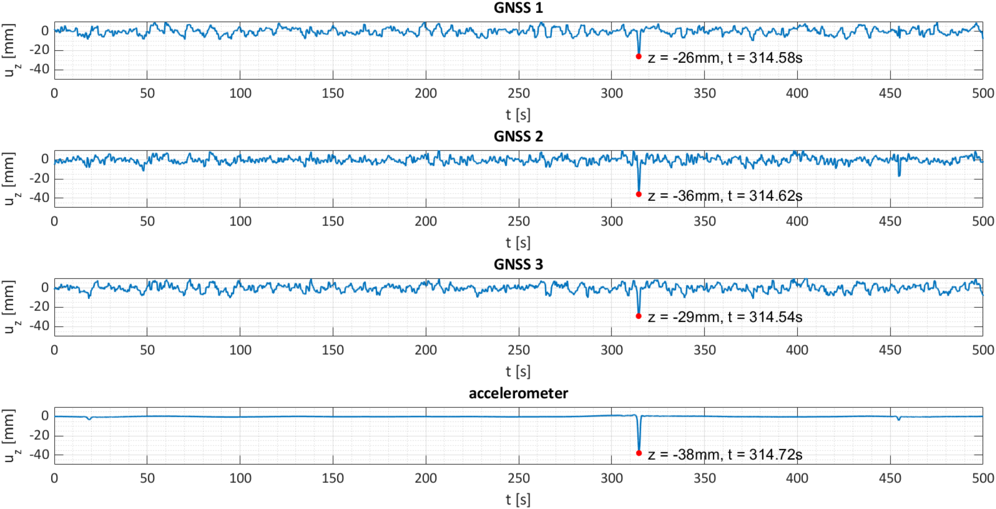
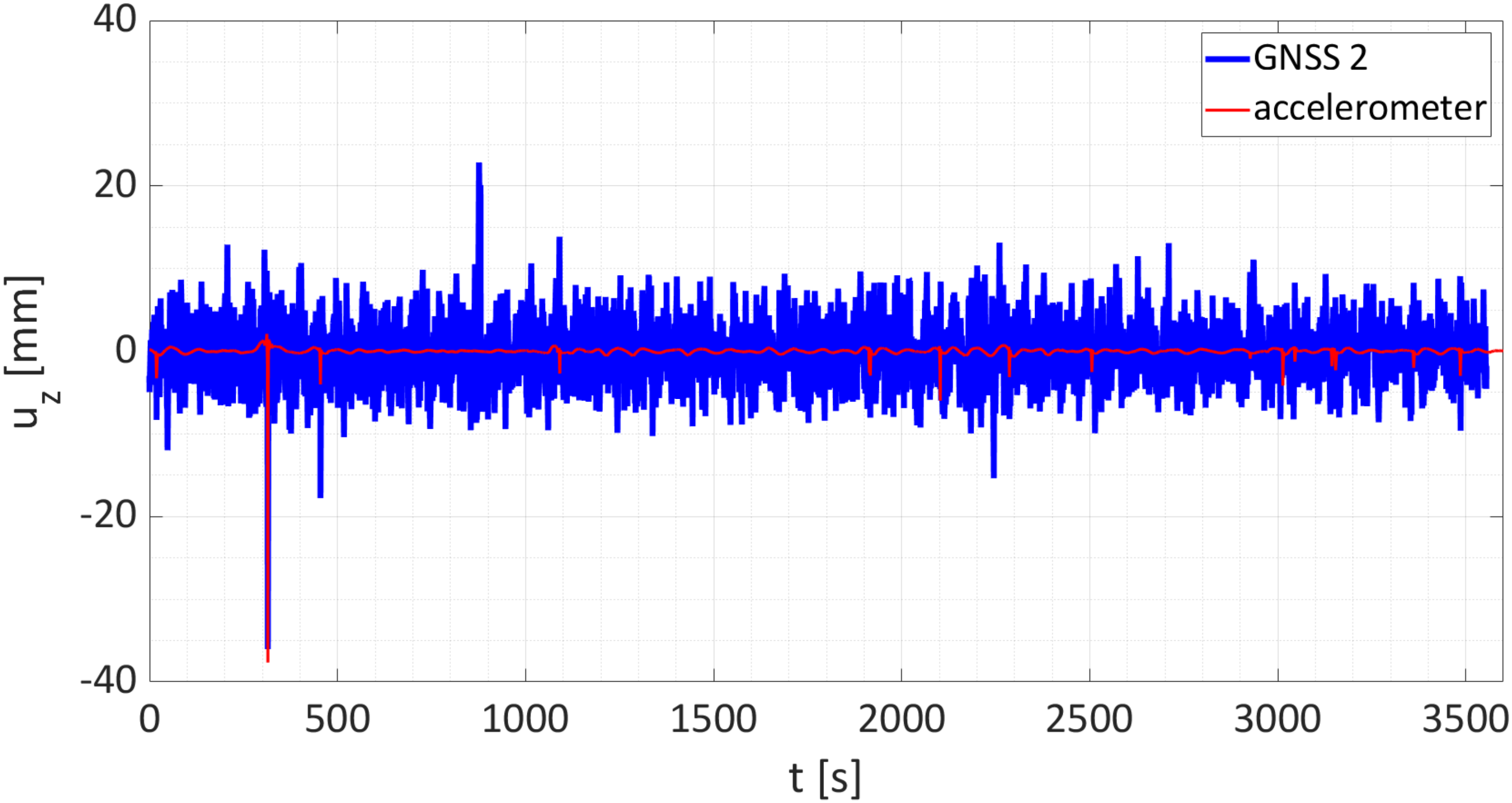
3.2. Validation
4. Discussion
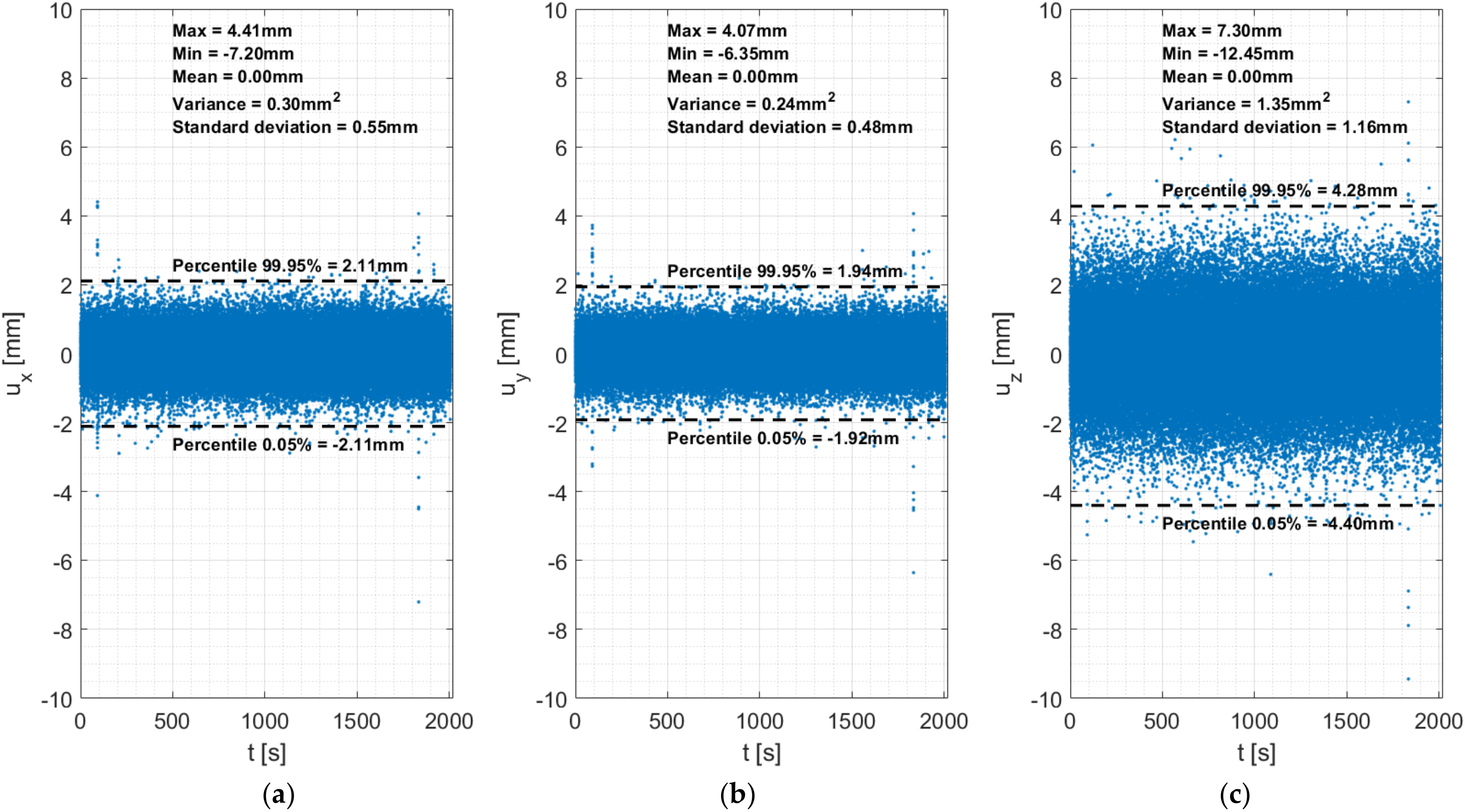
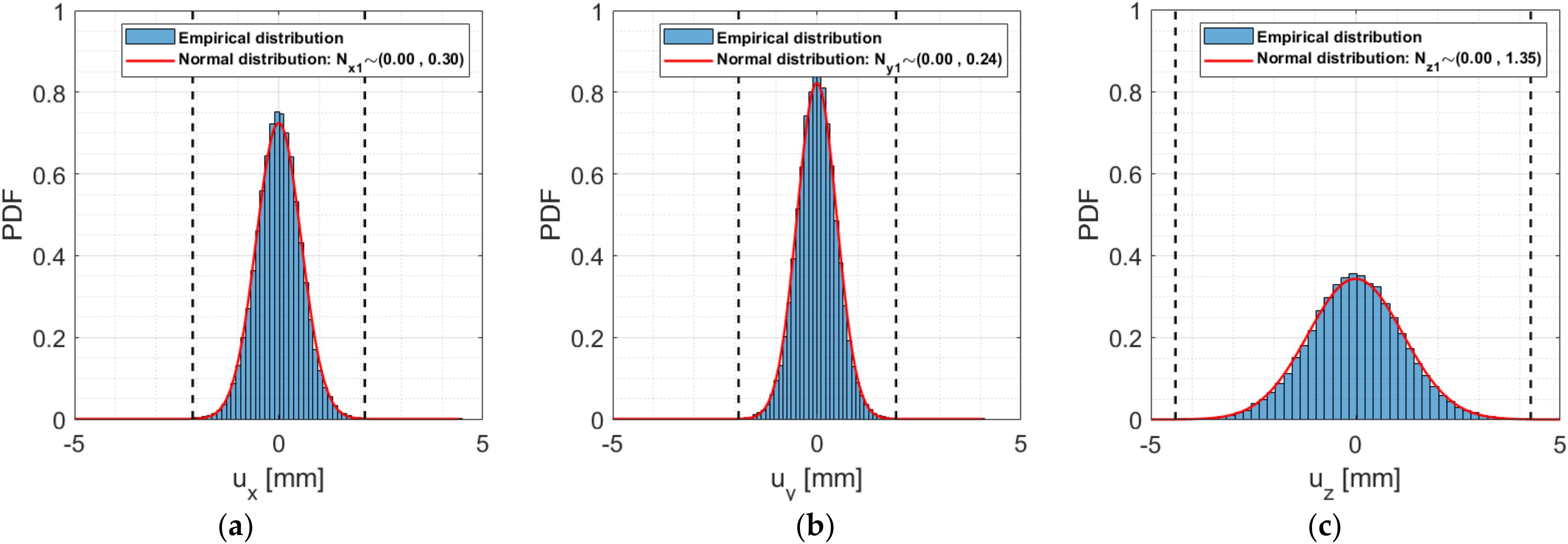
4.1. Statistical Analysis of the Noise of the GNSS Signal
4.1.1. Small Scale Benchmark Structure
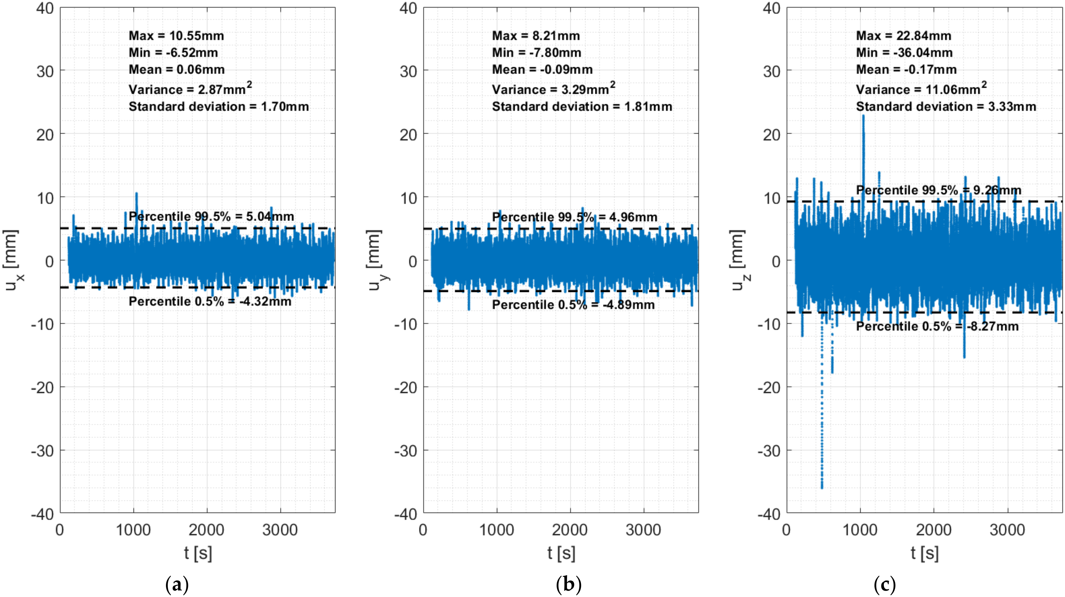
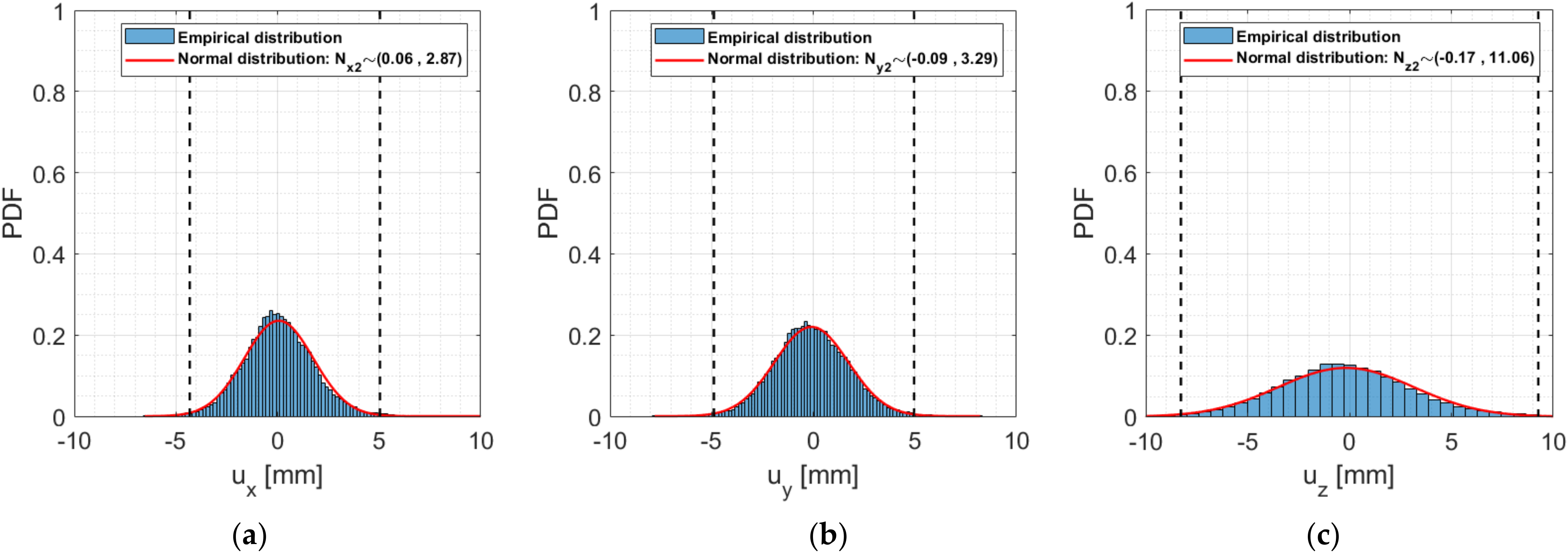
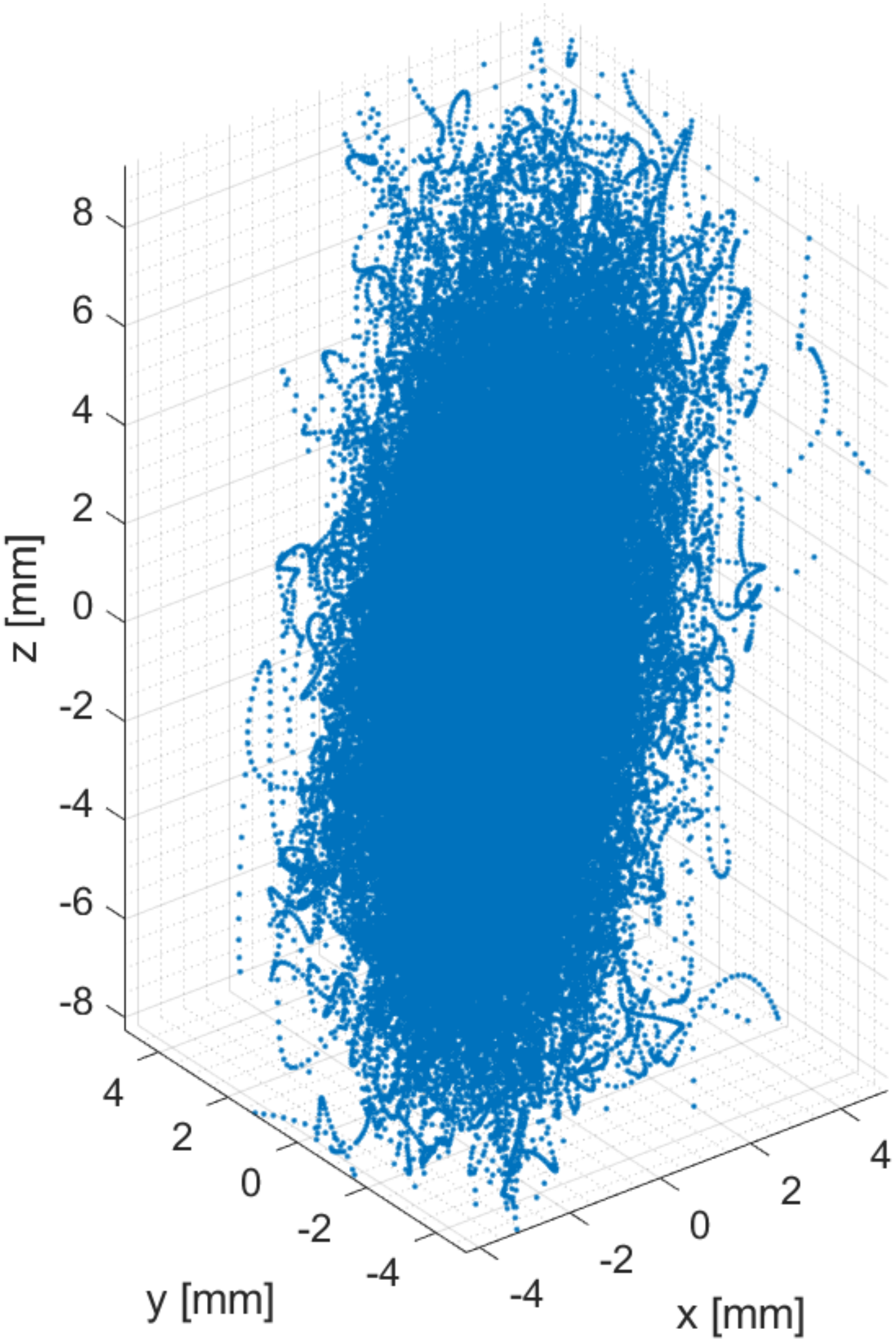
4.1.2. Road Bridge
Author Contributions
Funding
Institutional Review Board Statement
Informed Consent Statement
Data Availability Statement
Acknowledgments
Conflicts of Interest
References
- Larocca, A.P.C.; de Araújo Neto, J.O.; Trabanco, J.L.A.; dos Santos, M.C.; Barbosa, A.C.B. First Steps Using Two GPS Satellites for Monitoring the Dynamic Behavior of a Small Concrete Highway Bridge. J. Surv. Eng. 2016, 142, 04016008. [Google Scholar] [CrossRef]
- Moschas, F.; Stiros, S. Measurement of the dynamic displacements and of the modal frequencies of a short-span pedestrian bridge using GPS and an accelerometer. Eng. Struct. 2011, 33, 10–17. [Google Scholar] [CrossRef]
- Limongelli, M.P.; Çelebi, M. Seismic Structural Health Monitoring, 1st ed.; Springer: Cham, Switzerland, 2019. [Google Scholar]
- Rainieri, C.; Fabbrocino, G. Operational Modal Analysis of Civil Engineering Structures, 1st ed.; Springer: New York, NY, USA, 2014; Available online: https://link.springer.com/book/10.1007/978-1-4939-0767-0 (accessed on 29 June 2022).
- Kaloop, M.R.; Elbeltagi, E.; Wan Hu, J.; Elrefai, A. Recent Advances of Structures Monitoring and Evaluation Using GPS-Time Series Monitoring Systems: A Review. Int. J. Geo Inf. 2017, 6, 382. [Google Scholar] [CrossRef]
- Li, X.; Wang, B.; Li, X.; Huang, J.; Lyu, H.; Han, X. Principle and performance of multi-frequency and multi-GNSS PPP-RTK. Satell. Navig. 2022, 3, 1–11. [Google Scholar] [CrossRef]
- Katsigianni, G.; Loyer, S.; Perosanz, F. PPP and PPP-AR Kinematic Post-Processed Performance of GPS-Only, Galileo-Only and Multi-GNSS. Remote Sens. 2019, 11, 2477. [Google Scholar] [CrossRef]
- Glaner, M.; Weber, R. PPP with integer ambiguity resolution for GPS and Galileo using satellite products from different analysis centers. GPS Solut. 2021, 25, 1–13. [Google Scholar]
- European GNSS Agency. PPP-RTK Market and Technology Report. 2019. Available online: https://www.euspa.europa.eu/simplecount_pdf/tracker?file=calls_for_proposals/rd.03_-_ppp-rtk_market_and_technology_report.pdf (accessed on 29 June 2022).
- Fu, C.C.; Zhu, Y.; Hou, K.-Y. Utilization of Dynamic and Static Sensors for Monitoring Infrastructures. Adv. Remote Sensing Technology for Synthetic Aperture Radar Applications, Tsunami Disasters, and Infrastructure, 1st ed.; Marghany, M., Ed.; IntechOpen: London, UK, 2019; Available online: https://www.intechopen.com/chapters/65339 (accessed on 29 June 2022).
- Han, H.; Wang, J.; Meng, X.; Liu, H. Analysis of the dynamic response of a long span bridge using GPS/accelerometer/anemometer under typhoon loading. Eng. Struct. 2016, 122, 238–250. Available online: https://www.sciencedirect.com/science/article/abs/pii/S0141029616301602?via%3Dihub (accessed on 29 June 2022). [CrossRef]
- Capellari, G.; Chatzi, E.; Mariani, S. Cost–Benefit Optimization of Structural Health Monitoring Sensor Networks. Sensors 2018, 18, 2174. [Google Scholar] [CrossRef] [PubMed]
- Kaloop, M.R.; Li, H. Multi input-single output models identification of tower bridge movements using GPS monitoring system. Meas. J. Int. Meas. Confed. 2014, 47, 531–539. Available online: https://www.sciencedirect.com/science/article/abs/pii/S0263224113004843?via%3Dihub (accessed on 29 June 2022). [CrossRef]
- Notti, D.; Cina, A.; Manzino, A.; Colombo, A.; Bendea, I.H.; Mollo, P.; Giordan, D. Low-Cost GNSS Solution for Continuous Monitoring of Slope Instabilities Applied to Madonna Del Sasso Sanctuary (NW Italy). Sensors 2020, 20, 289. [Google Scholar] [CrossRef] [PubMed]
- Pehlivan, H. Frequency analysis of GPS data for structural health monitoring observations. Struct. Eng. Mech. 2018, 66, 185–193. [Google Scholar]
- Moschas, F.; Stiros, S. Dynamic Deflections of a Stiff Footbridge Using 100-Hz GNSS and Accelerometer Data. J. Surv. Eng. 2015, 141, 1–8. [Google Scholar] [CrossRef]
- Ozer Yigit, C.; Gurlek, E. Experimental testing of high-rate GNSS precise point positioning (PPP) method for detecting dynamic vertical displacement response of engineering structures. Geomat. Nat. Hazards Risk 2017, 8, 893–904. [Google Scholar] [CrossRef]
- Kaloop, M.R.; Hu, J.W.; Elbeltagi, E. Adjustment and assessment of the measurements of low and high sampling frequencies of GPS real-time monitoring of structural movement. ISPRS Int. J. Geo Inf. 2016, 5, 222. [Google Scholar] [CrossRef]
- Wang, X.; Zhao, Q.; Xi, R.; Li, C.; Li, G.; Li, L. Review of Bridge Structural Health Monitoring Based on GNSS: From Displacement Monitoring to Dynamic Characteristic Identification. IEEE Access 2021, 9, 80043–80065. Available online: https://ieeexplore.ieee.org/document/9440896 (accessed on 29 June 2022). [CrossRef]
- Portland State Aerospace Society. Conversion of Geodetic Coordinates to the Local Tangent Plane; McGraw Hill: Portland, OR, USA, 2007; Available online: https://archive.psas.pdx.edu/CoordinateSystem/Latitude_to_LocalTangent.pdf (accessed on 29 June 2022).
- Murray, C. Oracle Spatial, User’s Guide and Reference, Release 9.0.1; Part Number A88805-01. 2001. Available online: https://docs.oracle.com/cd/A91202_01/901_doc/appdev.901/a88805/sdo_cs_c.htm (accessed on 29 June 2022).
- Ruffhead, A.; Whiting, B.M. Introduction to Geodetic Datum Transformations and Their Reversibility; UEL ACE Surveying Working Paper, No 01/2020. 2020. Available online: https://www.researchgate.net/publication/339887497_Introduction_to_geodetic_datum_transformations_and_their_reversibility (accessed on 29 June 2022).
- Heiskanen, W.A.; Moritz, H. Physical Geodesy; Freeman, W.H. and Company: San Francisco, CA, USA, 1967; Available online: https://archive.org/details/HeiskanenMoritz1967PhysicalGeodesy/page/n191/mode/2up (accessed on 29 June 2022).
- Moschas, F.; Avallone, A.; Saltogianni, V.; Stiros, S.C. Strong motion displacement waveforms using 10-Hz precise point positioning GPS: An assessment based on free oscillation experiments. Earthq. Eng. Struct. Dyn. 2014, 43, 1853–1866. [Google Scholar] [CrossRef]
- Welch, P.D. The Use of Fast Fourier Transform for the Estimation of Power Spectra: A Method Based on Time Averaging Over Short, Modified Periodograms. IEEE Trans. Audio Electroacoust. 1967, 15, 70–73. Available online: https://ieeexplore.ieee.org/document/1161901 (accessed on 29 June 2022). [CrossRef] [Green Version]

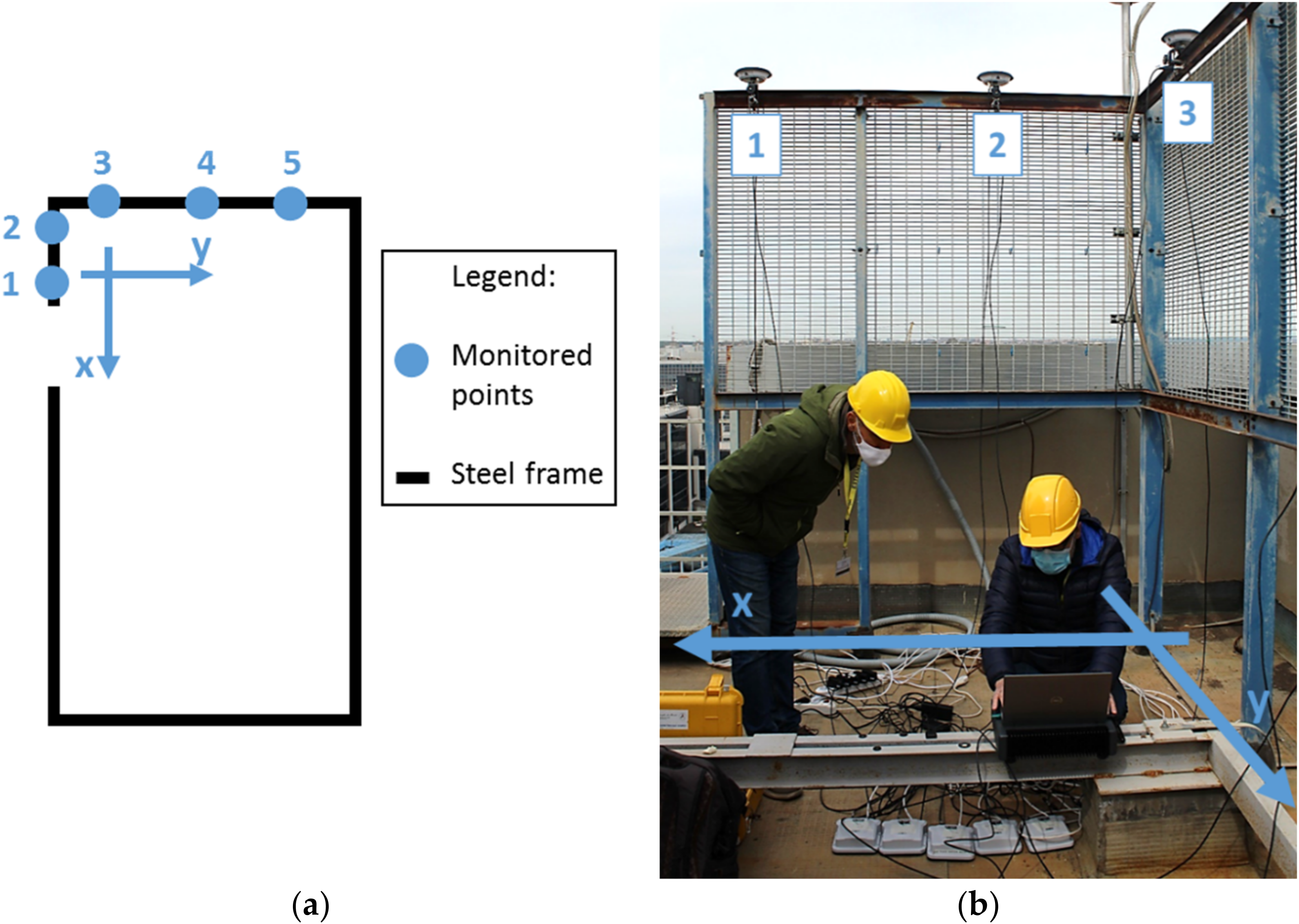
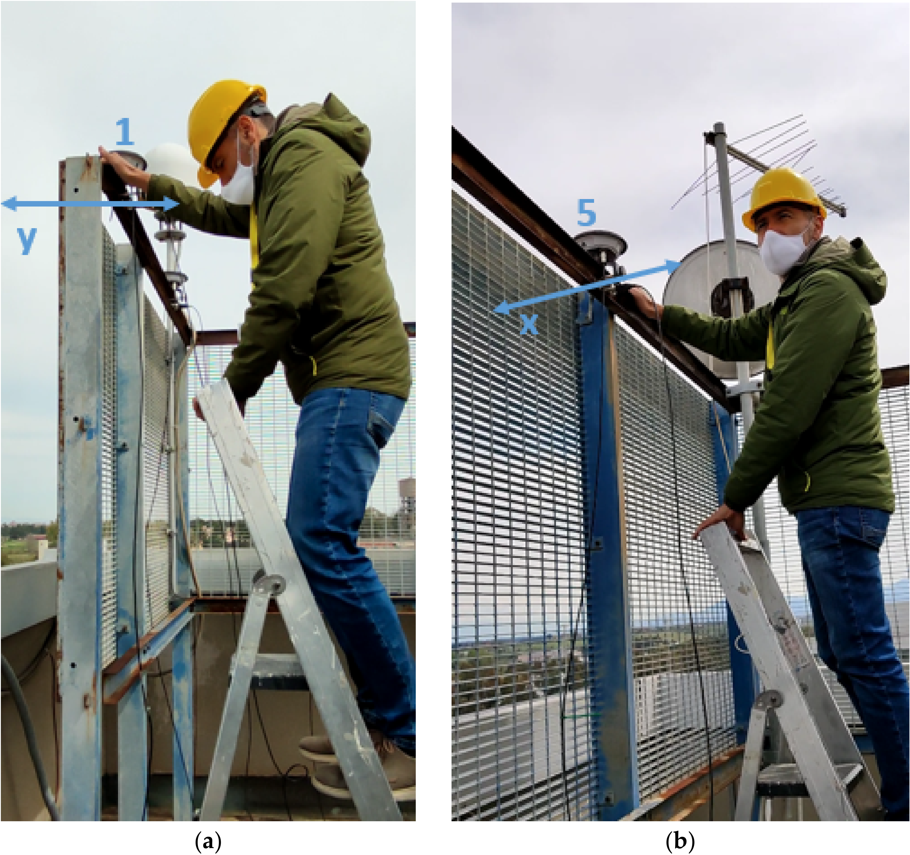
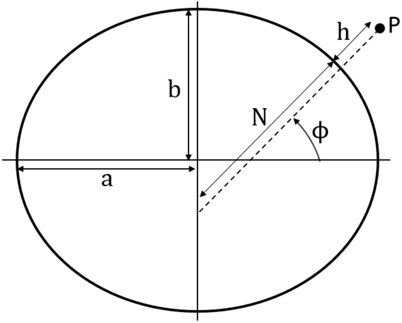

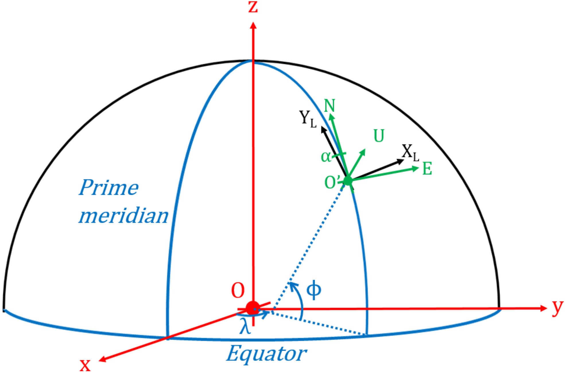
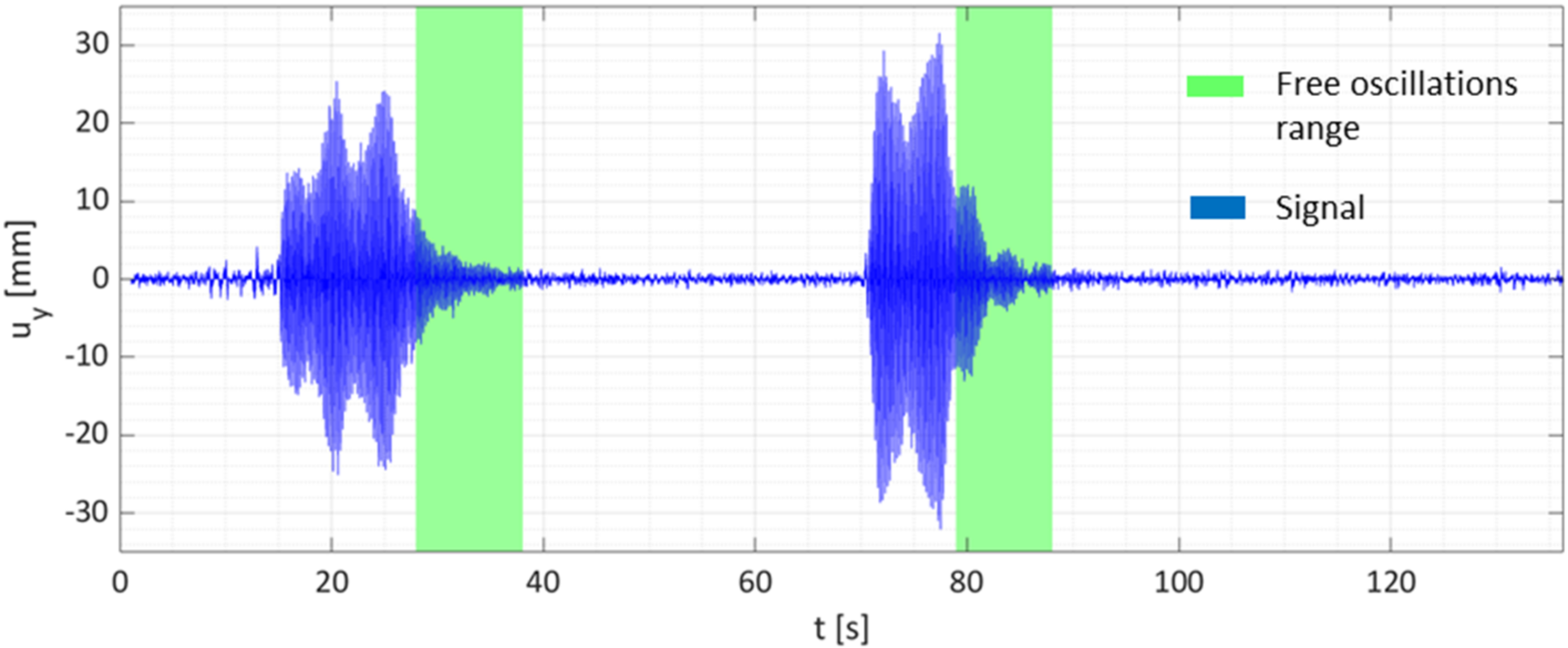
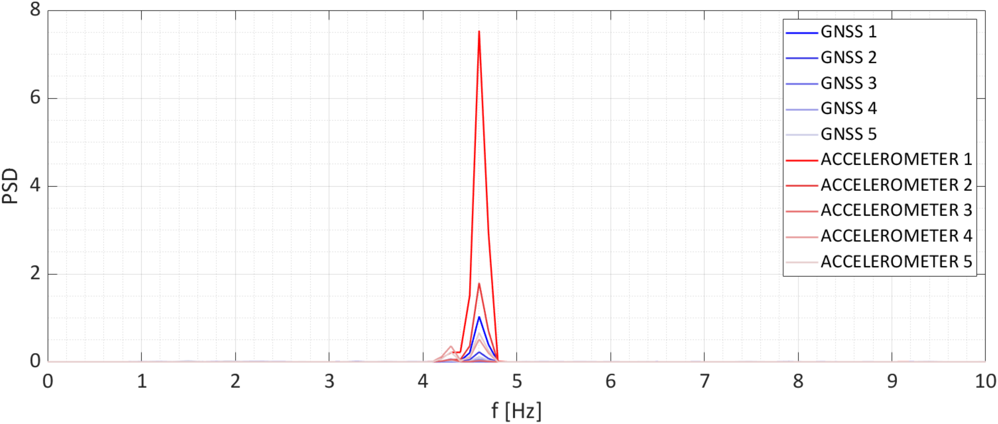
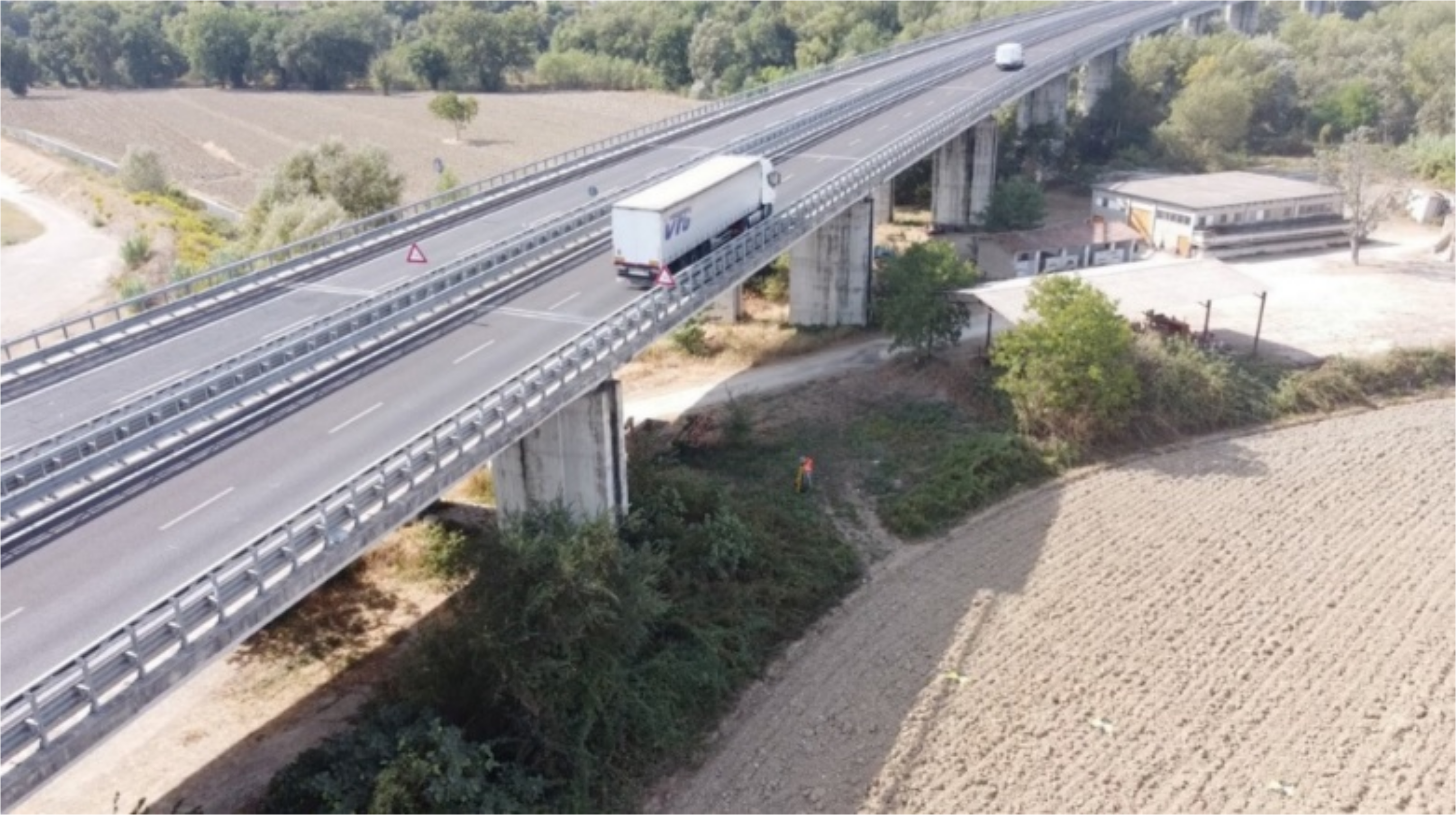

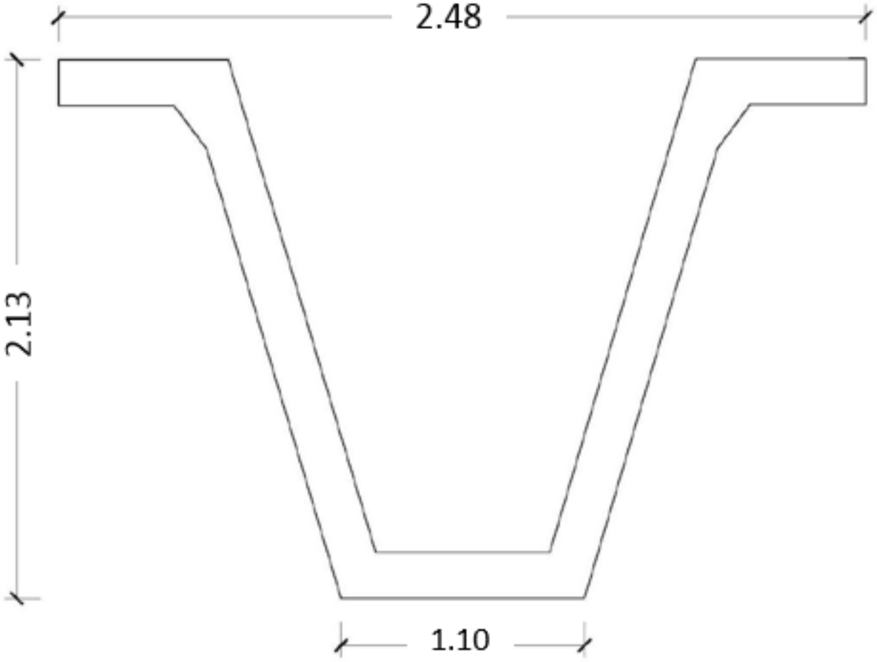

| Test | Direction of Excitation | Point of Application 1 |
|---|---|---|
| 1 | - | - |
| 2 | y | 1 |
| 3 | x | 5 |
| 4 | y | 1 |
| Name | Symbol | Value |
|---|---|---|
| Semimajor axis | a | 6,378,137 m |
| Semiminor axis | b | 6,356,752.31424518 m |
| Flatness | f | 3.3528107 × 10⁻³ |
| Eccentricity | e | 81.8191908 × 10⁻³ |
| Points | Peak Displacements [mm] | |||
|---|---|---|---|---|
| GNSS [mm] | Accelerometer [mm] | Difference [mm] | Percentage Difference [%] | |
| 1 | 25.4 | 18.7 | 6.7 | 26.4 |
| 2 | 13.2 | 8.9 | 4.3 | 32.6 |
| 3 | 5.8 | 3.4 | 2.4 | 41.4 |
| 4 | 12.8 | 9.1 | 3.7 | 28.9 |
| 5 | 14.6 | 9.9 | 4.7 | 32.2 |
| Mean values | 4.4 | 32.3 | ||
| Mean values without GNSS 3 | 4.9 | 30 | ||
| Points | Peak Frequencies | |||
|---|---|---|---|---|
| GNSS [Hz] | Accelerometer [Hz] | Difference [Hz] | Percentage Difference [%] | |
| 1 | 4.6 | 4.6 | 0.0 | 0.0 |
| 2 | 4.6 | 4.6 | 0.0 | 0.0 |
| 3 | 3.3 | 4.3 | 1.0 | 23.3 |
| 4 | 4.3 | 4.6 | 0.3 | 6.5 |
| 5 | 4.6 | 4.6 | 0.0 | 0.0 |
| Mean values | 4.28 | 4.54 | 0.26 | 6.0 |
| Mean values without GNSS 3 | 4.5 | 4.6 | 0.08 | 1.6 |
| Max | Min | Mean | Variance | Standard Deviation | Percentile 99.95% | Percentile 0.05% | Threshold | |
|---|---|---|---|---|---|---|---|---|
| [mm] | [mm] | [mm] | [mm2] | [mm] | [mm] | [mm] | [mm] | |
| x | 4.41 | −7.20 | 0.00 | 0.30 | 0.55 | 2.11 | −2.11 | +/−2.11 |
| y | 4.07 | −6.35 | 0.00 | 0.24 | 0.48 | 1.94 | −1.92 | +/−1.93 |
| z | 7.30 | −12.45 | 0.00 | 1.35 | 1.16 | 4.28 | −4.40 | +/−4.34 |
| Max | Min | Mean | Variance | Standard Deviation | Percentile 99.5% | Percentile 0.5% | Threshold | |
|---|---|---|---|---|---|---|---|---|
| [mm] | [mm] | [mm] | [mm2] | [mm] | [mm] | [mm] | [mm] | |
| x | 10.55 | −6.52 | 0.06 | 2.87 | 1.70 | 5.04 | −4.32 | +/− 4.68 |
| y | 8.21 | −7.80 | −0.09 | 3.29 | 1.81 | 4.96 | −4.89 | +/− 4.93 |
| z | 22.84 | −36.04 | −0.17 | 11.06 | 3.33 | 9.26 | −8.27 | +/− 8.77 |
Publisher’s Note: MDPI stays neutral with regard to jurisdictional claims in published maps and institutional affiliations. |
© 2022 by the authors. Licensee MDPI, Basel, Switzerland. This article is an open access article distributed under the terms and conditions of the Creative Commons Attribution (CC BY) license (https://creativecommons.org/licenses/by/4.0/).
Share and Cite
Cinque, D.; Saccone, M.; Capua, R.; Spina, D.; Falcolini, C.; Gabriele, S. Experimental Validation of a High Precision GNSS System for Monitoring of Civil Infrastructures. Sustainability 2022, 14, 10984. https://doi.org/10.3390/su141710984
Cinque D, Saccone M, Capua R, Spina D, Falcolini C, Gabriele S. Experimental Validation of a High Precision GNSS System for Monitoring of Civil Infrastructures. Sustainability. 2022; 14(17):10984. https://doi.org/10.3390/su141710984
Chicago/Turabian StyleCinque, Daniele, Mauro Saccone, Roberto Capua, Daniele Spina, Corrado Falcolini, and Stefano Gabriele. 2022. "Experimental Validation of a High Precision GNSS System for Monitoring of Civil Infrastructures" Sustainability 14, no. 17: 10984. https://doi.org/10.3390/su141710984
APA StyleCinque, D., Saccone, M., Capua, R., Spina, D., Falcolini, C., & Gabriele, S. (2022). Experimental Validation of a High Precision GNSS System for Monitoring of Civil Infrastructures. Sustainability, 14(17), 10984. https://doi.org/10.3390/su141710984


