
All-Sky Soil Moisture Estimation over Agriculture Areas from the Full Polarimetric SAR GF-3 Data


Abstract
:1. Introduction
2. Study Area and the Data Source
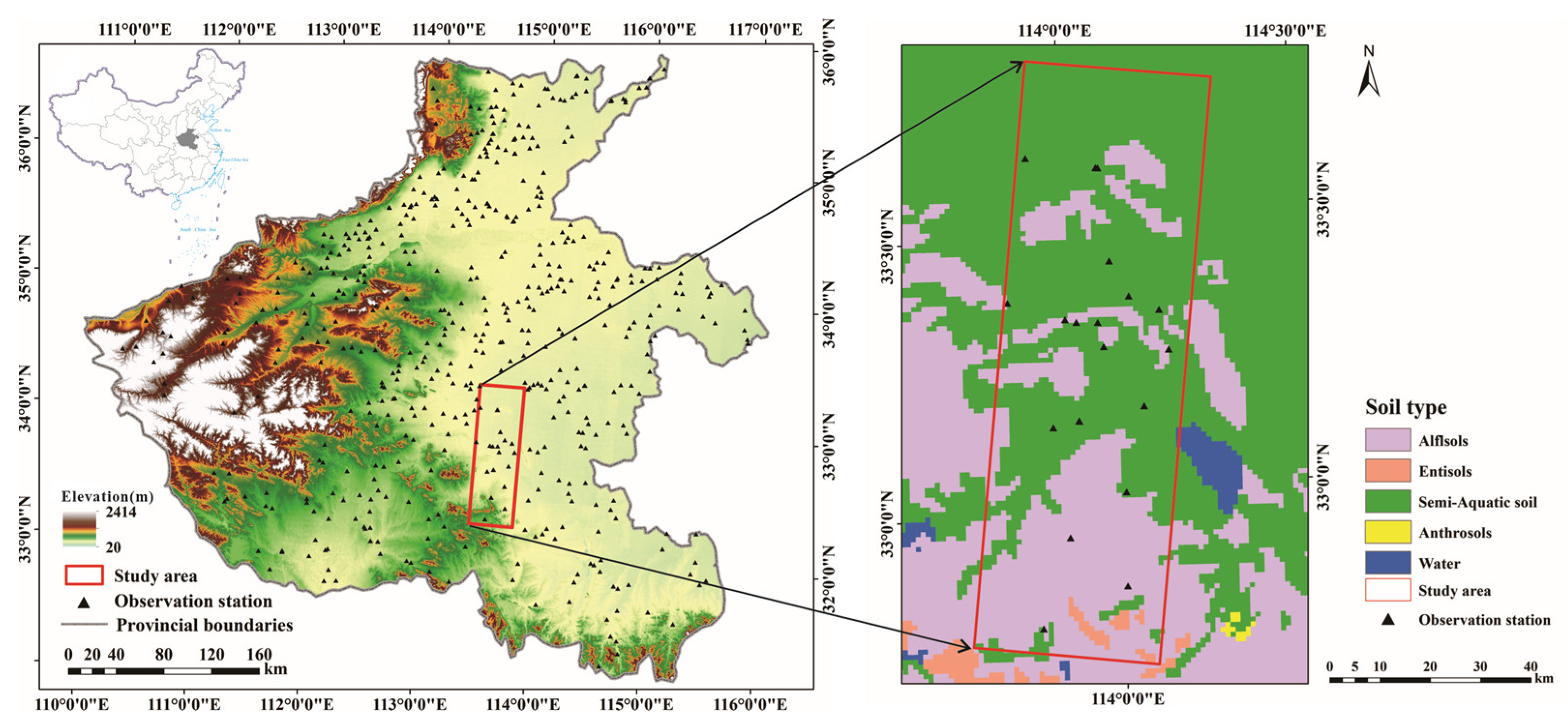
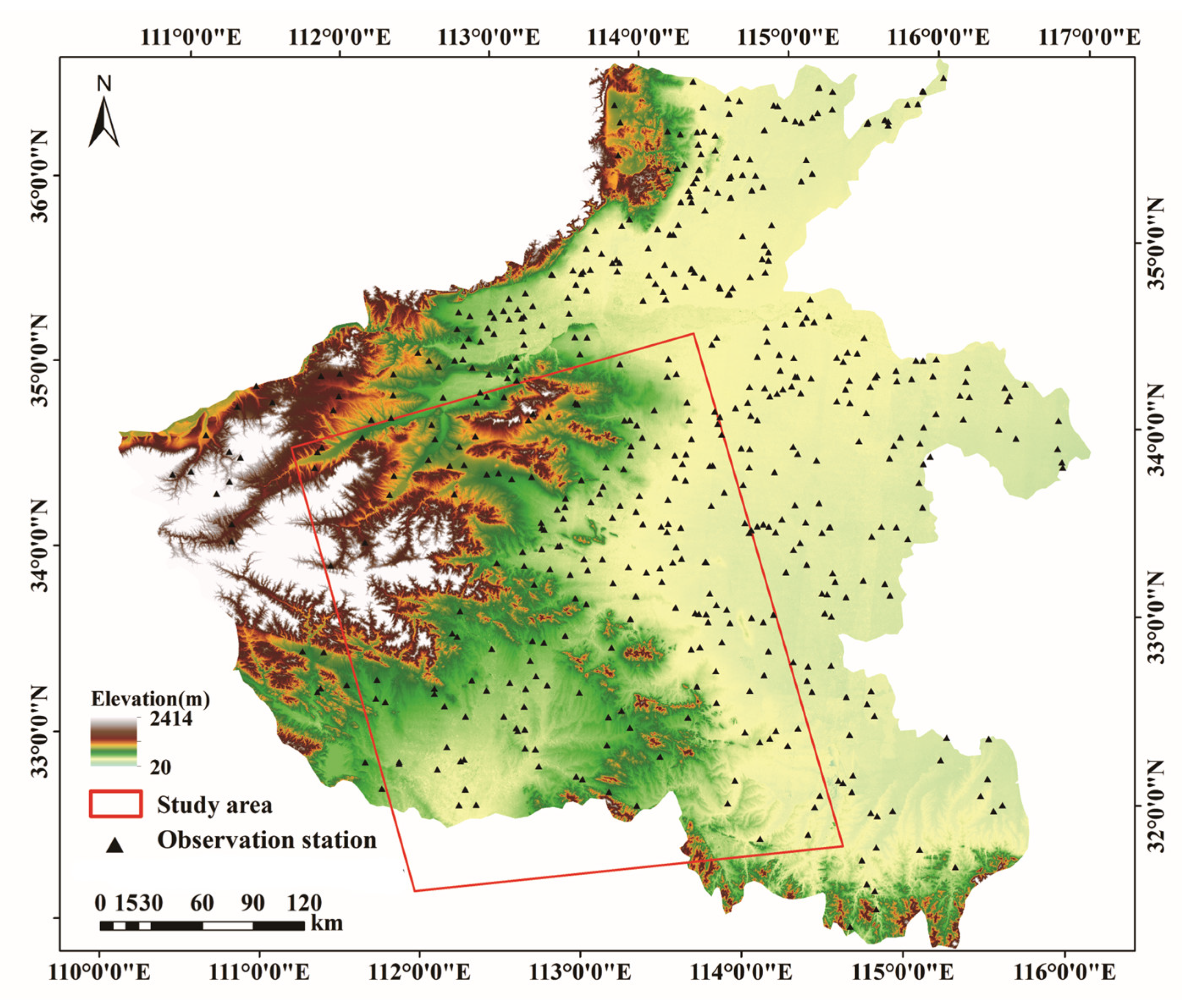
2.1. Study Area
2.2. Gaofen-3 (GF-3) Data
2.3. In Situ Measurements
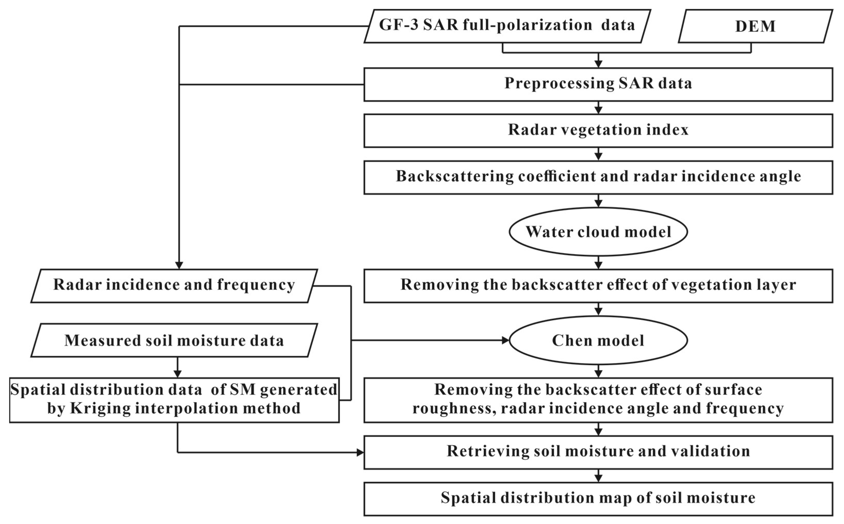
3. Methods
3.1. Radar Vegetation Index (RVI)
3.2. Water Cloud Model (WCM) and Chen Model
3.3. Validation
4. Results
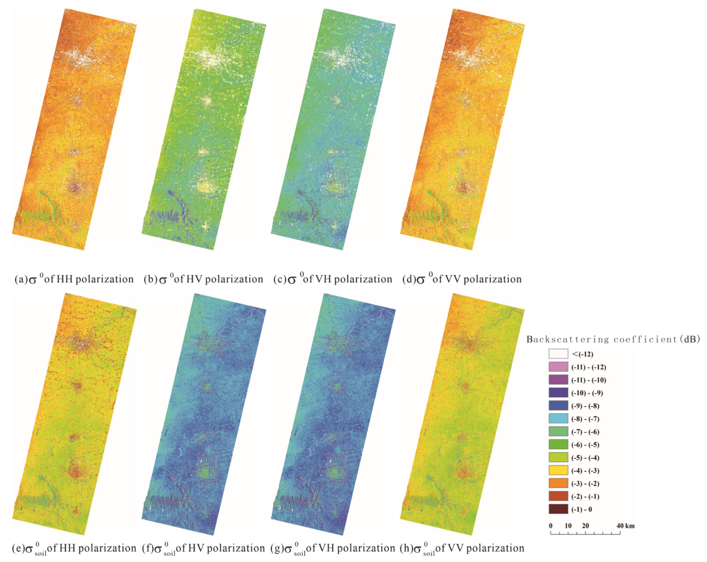
4.1. Soil Backscattering Coefficient ()
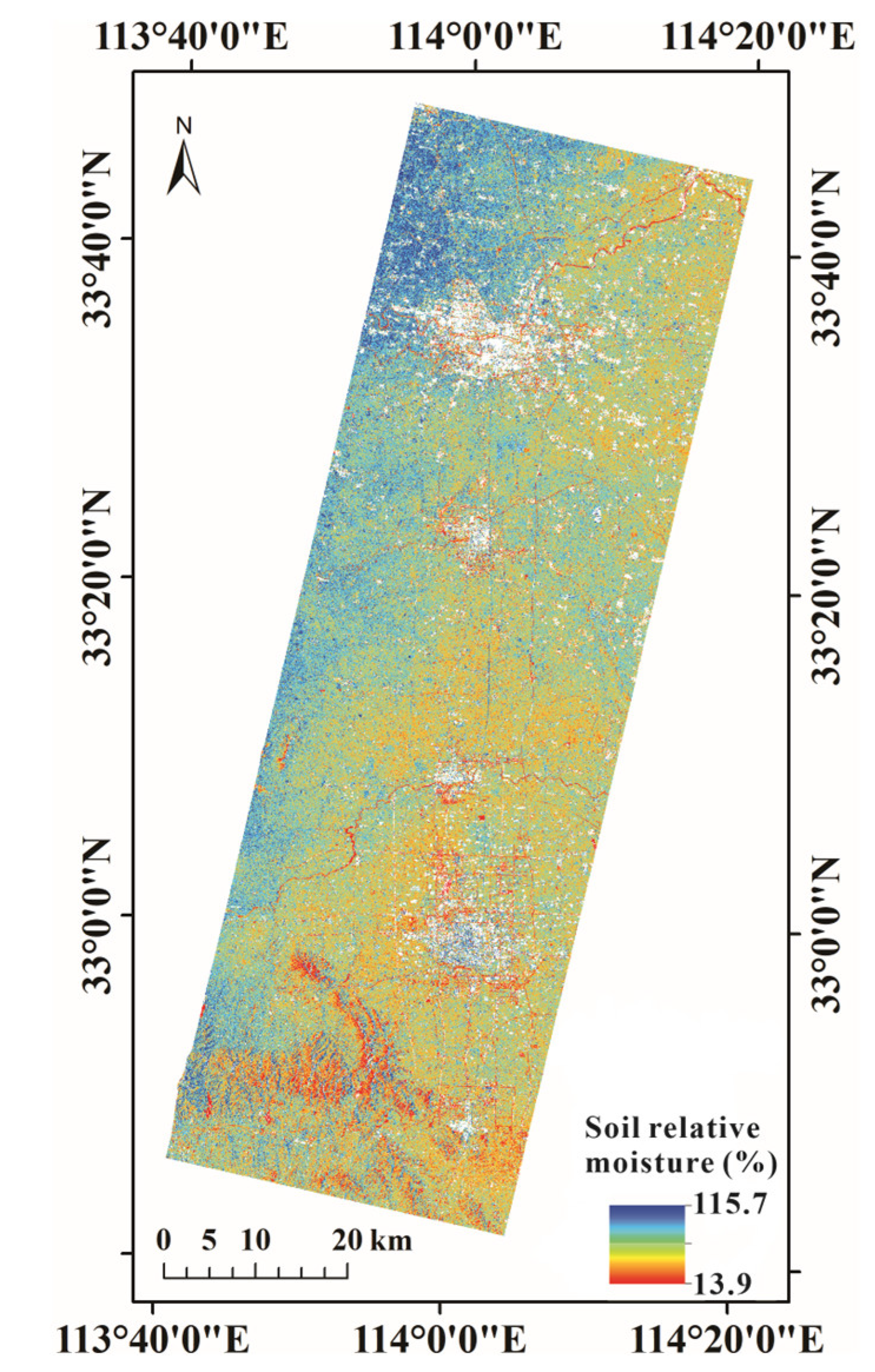
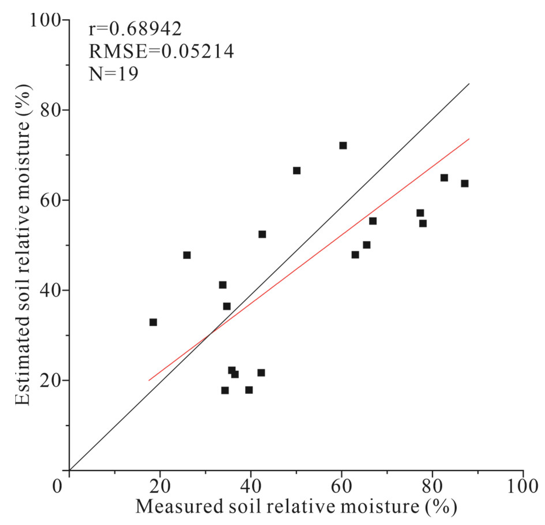
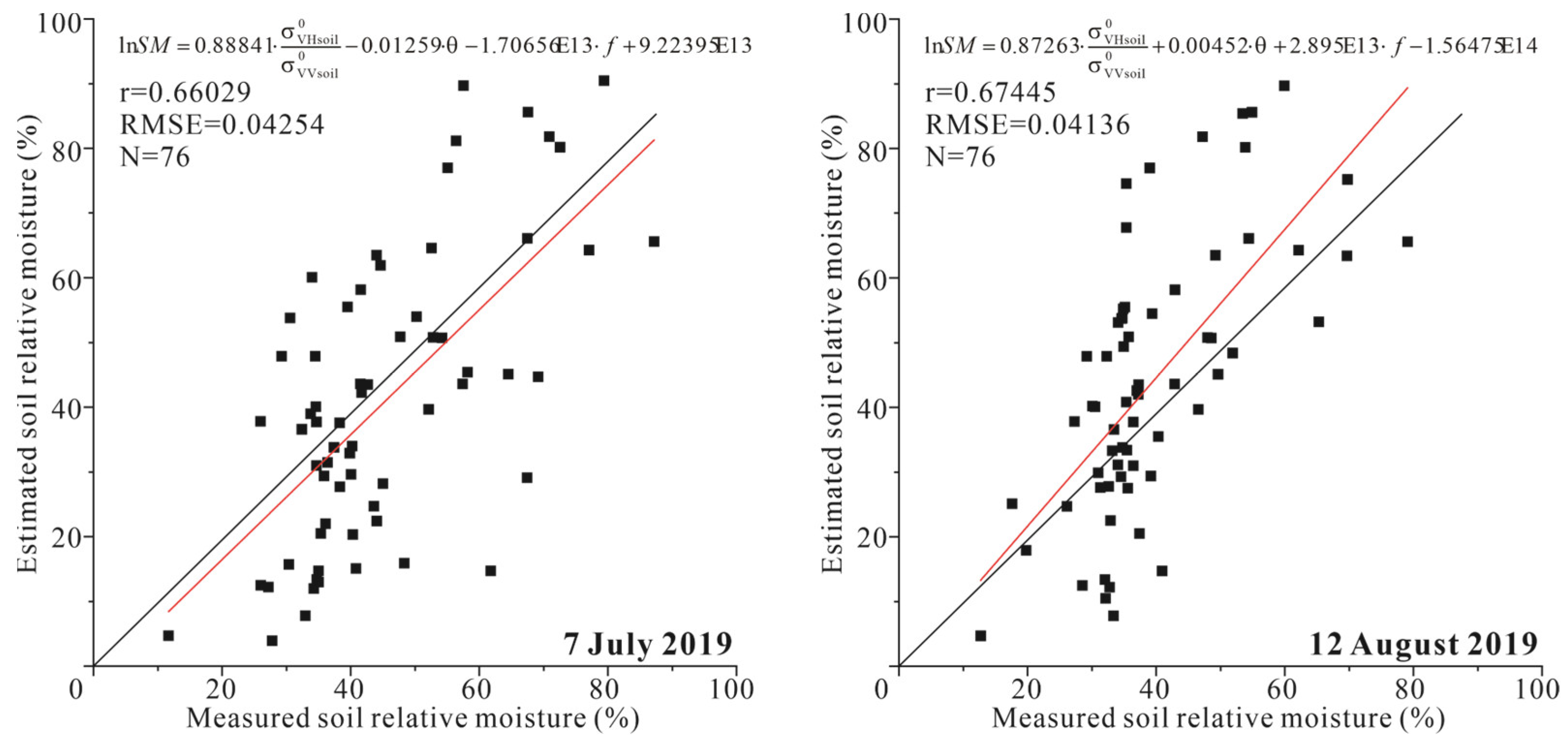
4.2. Soil Moisture Estimation and Verification
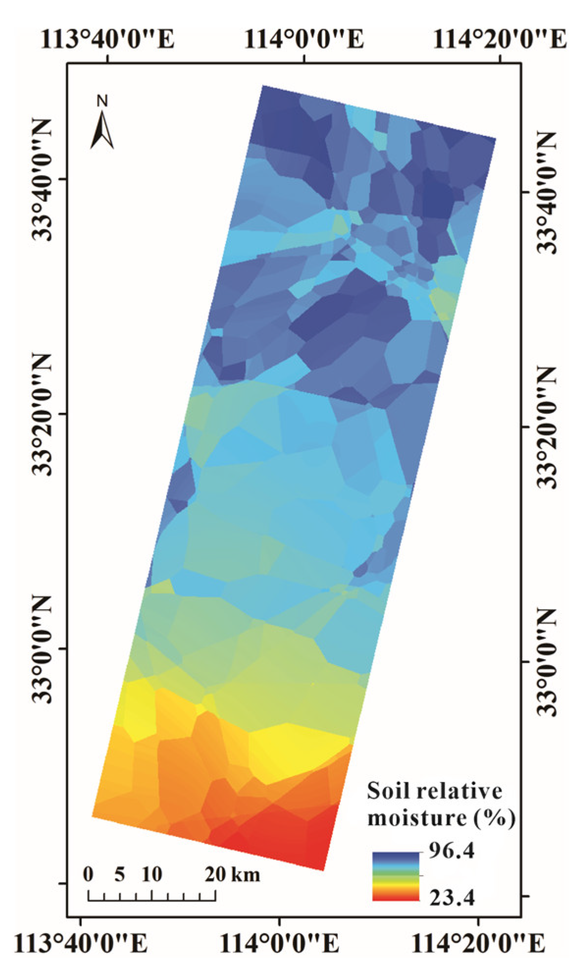
4.3. Extension of SM Estimation Model
5. Conclusions
Author Contributions
Funding
Institutional Review Board Statement
Informed Consent Statement
Data Availability Statement
Acknowledgments
Conflicts of Interest
References
- Seneviratne, S.I.; Corti, T.; Davin, E.L.; Hirschi, M.; Jaeger, E.B.; Lehner, I.; Orlowsky, B.; Teuling, A.J. Investigating soil moisture–climate interactions in a changing climate: A review. Earth Sci. Rev. 2010, 99, 125–161. [Google Scholar] [CrossRef]
- Bertoldi, G.; Chiesa, S.D.; Notarnicola, C.; Pasolli, L.; Niedrist, G.; Tappeiner, U. Estimation of soil moisture patterns in mountain grasslands by means of sar radarsat2 images and hydrological modeling. J. Hydrol. 2014, 516, 245–257. [Google Scholar] [CrossRef]
- Lin, H.; Chen, J.; Pei, Z.; Zhang, S.; Hu, X. Monitoring sugarcane growth using ENVISAT ASAR data. IEEE Trans. Geosci. Remote Sens. 2009, 47, 2572–2580. [Google Scholar] [CrossRef]
- Balenzano, A.; Mattia, F.; Satalino, G.; Davidson, M.W. Dense temporal series of C and L-band SAR data for soil moisture retrieval over agricultural crops. IEEE J. Select. Top. Appl. Earth Obs. Remote Sens. 2011, 4, 439–450. [Google Scholar] [CrossRef]
- Champagne, C.; Berg, A.; McNairn, H.; Drewitt, G.; Huffman, T. Evaluation of soil moisture extremes for agricultural productivity in the Canadian prairies. Agric. For. Meteorol. 2012, 165, 1–11. [Google Scholar] [CrossRef]
- El Hajj, M.; Baghd, A.I.N.; Zribi, M.; Belaud, G.; Cheviron, B.; Courault, D.; Charron, F. Soil moisture retrieval over irrigated grassland using x-band sar data. Remote Sens. Environ. 2016, 176, 202–218. [Google Scholar] [CrossRef]
- Gao, Q.; Zribi, M.; Escorihuela, M.J.; Baghdadi, N. Synergetic use of Sentinel-1 and Sentinel-2 data for soil moisture mapping at 100 m resolution. Sensors 2017, 17, 1966. [Google Scholar] [CrossRef]
- Mattia, F.; Satalino, G.; Pauwels, V.; Loew, A. Soil moisture retrieval through a merging of multi-temporal L-band SAR data and hydrologic modelling. Hydrol. Earth Syst. Sci. 2009, 13, 343–356. [Google Scholar] [CrossRef]
- Dey, S.; Mandal, D.; Robertson, L.D.; Banerjee, B.; Kumar, V.; McNairn, H.; Bhattacharya, A.; Rao, Y. In-season crop classification using elements of the kennaugh matrix derived from polarimetric radarsat-2 sar data. Int. J. Appl. Earth Obs. Geoinf. 2020, 88, 102059. [Google Scholar] [CrossRef]
- Rahman, M.M.; Moran, M.S.; Thoma, D.P.; Bryant, R.; Collins, C.; Jackson, T.; Orr, B.; Tischler, M. Mapping surface roughness and soil moisture using multi-angle radar imagery without ancillary data. Remote Sens. Environ. 2008, 112, 391–402. [Google Scholar] [CrossRef]
- Wei, J.; Li, P.; Yang, J.; Zhang, J.; Lang, F. A new automatic ship detection method using L-band polarimetric SAR imagery. IEEE J. Select. Top. Appl. Earth Obs. Remote Sens. 2014, 7, 1383–1393. [Google Scholar] [CrossRef]
- Shi, H.; Zhao, L.; Yang, J.; Lopez-Sanchez, J.M.; Zhao, J.; Sun, W.; Shi, L.; Li, P. Soil moisture retrieval over agricultural fields from l-band multi-incidence and multitemporal polsar observations using polarimetric decomposition techniques. Remote Sens. Environ. 2021, 261, 112485. [Google Scholar] [CrossRef]
- Aubert, M.; Baghdadi, N.; Zribi, M.; Douaoui, A.; Garrigues, S. Analysis of terrasar-x data sensitivity to bare soil moisture, roughness, composition and soil crust. Remote Sens. Environ. 2011, 115, 1801–1810. [Google Scholar] [CrossRef]
- Doubková, M.; Van Dijk, A.I.J.M.; Sabel, D.; Wagner, W.; Blöschl, G. Evaluation of the predicted error of the soil moisture retrieval from c-band sar by comparison against modelled soil moisture estimates over australia. Remote Sens. Environ. 2012, 120, 188–196. [Google Scholar] [CrossRef]
- Bauer-Marschallinger, B.; Freeman, V.; Cao, S.; Paulik, C.; Schaufler, S.; Stachl, T.; Modanesi, S.; Massari, C.; Ciabatta, L.; Brocca, L.; et al. Toward global soil moisture monitoring with Sentinel-1: Harnessing assets and overcoming obstacles. IEEE Trans. Geosci. Remote Sens. 2018, 57, 520–539. [Google Scholar] [CrossRef]
- Wang, J.; Wu, F.; Shang, J.; Zhou, Q.; Ahmad, I.; Zhou, G. Saline soil moisture mapping using Sentinel-1A synthetic aperture radar data and machine learning algorithms in humid region of China’s east coast. Catena 2022, 213, 106189. [Google Scholar] [CrossRef]
- Fung, A.K.; Li, Z.; Chen, K.S. Backscattering from a randomly rough dielectric surface. IEEE Trans. Geosci. Remote Sens. 1992, 30, 356–369. [Google Scholar] [CrossRef]
- Dubois, P.C.; Van Zyl, J.; Engman, T. Measuring soil moisture with imaging radars. IEEE Trans. Geosci. Remote Sens. 2002, 33, 915–926. [Google Scholar] [CrossRef]
- Oh, Y. Quantitative retrieval of soil moisture content and surface roughness from multipolarized radar observations of bare soil surfaces. IEEE Trans. Geosci. Remote Sens. 2004, 42, 596–601. [Google Scholar] [CrossRef]
- Chen, K.S.; Wu, T.D.; Tsang, L.; Li, Q.; Shi, J.; Fung, A.K. Emission of Rough Surfaces Calculated by the Integral Equation Method with Comparison to ThreeDimensional Moment Method Simulations. IEEE Trans. Geosci. Remote Sens. 2003, 41, 90–101. [Google Scholar] [CrossRef]
- Loew, A.; Mauser, W. A semiempirical surface backscattering model for bare soil surfaces based on a generalized power law spectrum approach. IEEE Trans. Geosci. Remote Sens. 2006, 44, 1022–1035. [Google Scholar] [CrossRef]
- Chen, S.K.; Yen, S.K.; Huang, W.P. A simple model for retrieving bare soil moisture from radar-scattering coefficients. Remote Sens. Environ. 1995, 54, 121–126. [Google Scholar] [CrossRef]
- Ulaby, F.T.; Sarabandi, K.; McDonald, K.; Whitt, M.; Dobson, M.C. Michigan Microwave Canopy Scattering Model. Int. J. Remote Sens. 1990, 11, 1223–1253. [Google Scholar] [CrossRef]
- Attema, E.P.W.; Ulaby, F.T. Vegetation modeled as a water cloud. Radio Sci. 1978, 13, 357–364. [Google Scholar] [CrossRef]
- Baghdadi, N.N.; El Hajj, M.; Zribi, M.; Fayad, I. Coupling SAR C-band and optical data for soil moisture and leaf area index retrieval over irrigated grasslands. IEEE J. Select. Top. Appl. Earth Obs. Remote Sens. 2015, 9, 1229–1243. [Google Scholar] [CrossRef]
- El Hajj, M.; Baghdadi, N.; Zribi, M.; Bazz, H. Synergic use of Sentinel-1 and Sentinel-2 images for operational soil moisture mapping at high spatial resolution over agricultural areas. Remote Sens. 2017, 9, 1292. [Google Scholar] [CrossRef]
- He, B.; Xing, M.; Bai, X. A synergistic methodology for soil moisture estimation in an alpine prairie using radar and optical satellite data. Remote Sens. 2014, 6, 10966–10985. [Google Scholar] [CrossRef]
- Jagdhuber, T.; Hajnsek, I.; Papathanassiou, K.P. An iterative generalized hybrid decomposition for soil moisture retrieval under vegetation cover using fully polarimetric SAR. IEEE J. Select. Top. Appl. Earth Obs. Remote Sens. 2014, 8, 3911–3922. [Google Scholar] [CrossRef]
- Hajnsek, I.; Jagdhuber, T.; Schon, H.; Papathanassiou, K.P. Potential of estimating soil moisture under vegetation cover by means of polsar. IEEE Trans. Geosci. Remote Sens. 2009, 47, 442–454. [Google Scholar] [CrossRef]
- Wang, Z.; Zhao, T.; Qiu, J.; Zhao, X.; Li, R.; Wang, S. Microwave-based vegetation descriptors in the parameterization of water cloud model at L-band for soil moisture retrieval over croplands. GISci. Remote Sens. 2020, 58, 48–67. [Google Scholar] [CrossRef]
- Zheng, X.; Feng, Z.; Li, L.; Li, B.; Chen, S. Simultaneously estimating surface soil moisture and roughness of bare soils by combining optical and radar data. Int. J. Appl. Earth Obs. Geoinf. 2021, 100, 102345. [Google Scholar] [CrossRef]
- Lievens, H.; Verhoest, N.E. On the retrieval of soil moisture in wheat fields from Lband SAR based on water cloud modeling, the IEM, and effective roughness parameters. IEEE Geosci. Remote Sens. Lett. 2011, 8, 740–744. [Google Scholar] [CrossRef]
- Li, J.; Wang, S. Using SAR-derived vegetation descriptors in a water cloud model to improve soil moisture retrieval. Remote Sens. 2018, 10, 1370. [Google Scholar] [CrossRef]
- Kim, Y. Radar vegetation index for estimating the vegetation water content of rice and soybean. IEEE Geosci. Remote Sens. Lett. 2012, 9, 564–568. [Google Scholar] [CrossRef]
- Mandal, D.; Kumar, V.; Ratha, D.; Dey, S.; Bhattacharya, A.; Lopez-Sanchez, J.M.; McNairn, H.; Rao, Y.S. Dual polarimetric radar vegetation index for crop growth monitoring using Sentinel-1 SAR data. Remote Sens. Environ. 2020, 247, 111954. [Google Scholar] [CrossRef]
- Liang, J.; Liang, G.; Zhao, Y.; Zhang, Y. A synergic method of Sentinel-1 and Sentinel-2 images for retrieving soil moisture content in agricultural regions. Comput. Electron. Agric. 2021, 190, 106485. [Google Scholar] [CrossRef]
- Pierdicca, N.; Pulvirenti, L.; Bignami, C. Soil moisture estimation over vegetated terrains using multitemporal remote sensing data. Remote Sens. Environ. 2010, 114, 440–448. [Google Scholar] [CrossRef]
- Prakash, R.; Singh, D.; Pathak, N.P. A fusion approach to retrieve soil moisture with sar and optical data. IEEE J. Sel. Top. Appl. Earth Obs. Remote Sens. 2012, 5, 196–206. [Google Scholar] [CrossRef]
- Zhu, Y.; Liu, K.; Myint, S.W.; Du, Z.; Li, Y.; Cao, J.; Liu, L.; Wu, Z. Integration of GF2 Optical, GF3 SAR, and UAV Data for Estimating Aboveground Biomass of China’s Largest Artificially Planted Mangroves. Remote Sens. 2020, 12, 2039. [Google Scholar] [CrossRef]
- Wang, M.; Wang, Y.; Run, Y.; Chen, Y.; Jin, S. Geometric Accuracy Analysis for GaoFen3 Stereo Pair Orientation. IEEE Geosci. Remote Sens. Lett. 2017, 15, 92–96. [Google Scholar] [CrossRef]
- Wu, Y.; Fan, B.; Wang, J. Design and implementation of Henan meteorological observation station network management system. Sci. Technol. Inf. 2019, 17, 20–26. [Google Scholar] [CrossRef]
- Fan, B. Design and Implenentation of Henan Provincial Meteoological Ohsevation Data Service Platform. Meteool. Environ. Sci. 2019, 42, 135–142. [Google Scholar] [CrossRef]
- Kim, Y.; Van, Z.J.J. A Time-Series Approach to Estimate Soil Moisture Using Polarimetric Radar Data. IEEE Trans. Geosci. Remote Sens. 2009, 47, 2519–2527. [Google Scholar] [CrossRef]
- Singh, G.; Das, N.N.; Panda, R.K.; Mohanty, B.P.; Entekhabi, D.; Bhattacharya, B.K. Yueh. Soil Moisture Retrieval Using SMAP L-Band Radiometer and RISAT-1 C-Band SAR Data in the Paddy Dominated Tropical Region of India. IEEE J. Sel. Top. Appl. Earth Obs. Remote Sens. 2021, 14, 10644–10664. [Google Scholar] [CrossRef]
- Singh, G.; Das, N.N.; Panda, R.K.; Colliander, A.; Jackson, T.J.; Mohanty, B.P.; Entekhabi, D.; Simon, H. Yueh. Validation of SMAP Soil Moisture Products Using Ground-Based Observations for the Paddy Dominated Tropical Region of India. IEEE Trans. Geosci. Remote Sens. 2019, 57, 8479–8491. [Google Scholar] [CrossRef]
- Tolometti, G.D.; Neish, C.D.; Hamilton, C.W.; Osinski, G.R.; Kukko, A.; Voigt, J.R.C. Differentiating Fissure-Fed Lava Flow Types and Facies Using RADAR and LiDAR: An Example From the 2014–2015 Holuhraun Lava Flow-Field. J. Geophys. Res. Solid Earth 2022, 127, e2021JB023419. [Google Scholar] [CrossRef]
- Singh, A.; Gaurav, K.; Rai, A.K.; Beg, Z. Machine Learning to Estimate Surface Roughness from Satellite Images. Remote Sens. 2021, 13, 3794. [Google Scholar] [CrossRef]


| Backscattering Coefficient | HH | HV | VH | VV |
|---|---|---|---|---|
| Backscattering coefficient () | 0.3860 | 0.2941 | 0.3703 | 0.5874 |
| Soil backscattering coefficient () | 0.4235 | 0.3089 | 0.4163 | 0.6084 |
Publisher’s Note: MDPI stays neutral with regard to jurisdictional claims in published maps and institutional affiliations. |
© 2022 by the authors. Licensee MDPI, Basel, Switzerland. This article is an open access article distributed under the terms and conditions of the Creative Commons Attribution (CC BY) license (https://creativecommons.org/licenses/by/4.0/).
Share and Cite
Luo, D.; Wen, X.; Xu, J. All-Sky Soil Moisture Estimation over Agriculture Areas from the Full Polarimetric SAR GF-3 Data. Sustainability 2022, 14, 10866. https://doi.org/10.3390/su141710866
Luo D, Wen X, Xu J. All-Sky Soil Moisture Estimation over Agriculture Areas from the Full Polarimetric SAR GF-3 Data. Sustainability. 2022; 14(17):10866. https://doi.org/10.3390/su141710866
Chicago/Turabian StyleLuo, Dayou, Xingping Wen, and Junlong Xu. 2022. "All-Sky Soil Moisture Estimation over Agriculture Areas from the Full Polarimetric SAR GF-3 Data" Sustainability 14, no. 17: 10866. https://doi.org/10.3390/su141710866
APA StyleLuo, D., Wen, X., & Xu, J. (2022). All-Sky Soil Moisture Estimation over Agriculture Areas from the Full Polarimetric SAR GF-3 Data. Sustainability, 14(17), 10866. https://doi.org/10.3390/su141710866