A Modified SWAT Model to Simulate Soil Water Content and Soil Temperature in Cold Regions: A Case Study of the South Saskatchewan River Basin in Canada

Abstract

Soil water content (SWC) and soil temperature are important hydrologic state variables. Accurate model simulation is critical in hydrologic regimes in cold regions dominated by spring snowmelt. In this study, we developed a combined physically-based soil temperature and energy-balance rain-on-snow (ROS) module for the Soil and Water Assessment Tool (SWAT) model and applied it to the South Saskatchewan River Basin (SSRB). We calibrated the SWAT base (SWAT-B) model and the SWAT modified (SWAT–M) model using daily measured soil temperature and SWC by hydrological response unit (HRU) for the years 2015 to 2020. The results of sensitivity analysis using the SUFI-2 technique in SWAT-CUP indicated that eight parameters have the most significant (p < 0.5) effect on streamflow, soil moisture, and snowmelt. Statistics for the SWAT-B and SWAT-M streamflow models revealed that the new module improved the Nash-Sutcliffe efficiency (NSE) from 0.39 to 0.71 and 0.42 to 0.76 for calibration and validation, respectively. The statistics for SWAT-simulated daily SWC showed that the measured data were a better fit with SWAT-M versus the SWAT-B output. Furthermore, SWAT-B values exceeded SWAT-M output and field measurements, and thus, the range of SWAT-M results was a better fit with observations. SWAT-B tended to underestimate soil temperature in the cold season, while SWAT-M significantly improved soil temperature simulation for winter. This new SWAT module simulated freeze-thaw cycles and captured the influence of snow cover on surface soil ice-water content. Spatial analysis of SWC and soil temperature across the SSRB showed that the SWAT-M model predicted more SWC and lower soil temperature in the western part of SSRB than SWAT-B, with higher soil temperature and lower SWC in the eastern region.

1. Introduction

Soil water content (SWC) and soil temperature are important hydrologic state variables that play significant roles in controlling land surface processes and interacting with the atmosphere through evaporation and plant transpiration [1,2]. SWC is a critical link between the atmosphere and biosphere that affects the actual evapotranspiration (ET) from soil, plants and crops, surface runoff, subsurface interflow, and the recharging of groundwater [3,4]. Likewise, soil temperature affects crop growth during seed germination and plant emergence directly and indirectly through its influence on soil nutrient availability [5,6]. Therefore, spatial-temporal information for SWC and soil temperature inform soil management and conservation practices, particularly in sub-humid regions, such as the South Saskatchewan River Basin (SSRB). The SSRB is one of the major river systems in western Canada, extending from the headwaters in the Rocky Mountains in southwestern Alberta and across the prairie provinces of Alberta and Saskatchewan. Since most of Canada’s agricultural land is in this region [7], changes in SWC and/or soil temperature play a significant role in dryland crop production. Multi-year droughts occur periodically in the historical record [8,9] and prior to the instrumented period [10]. Several studies [11,12] have examined meteorological and agricultural drought in the Canadian prairies region, typically using drought indices, such as the Standardized Precipitation Index (SPI) and the Standardized Precipitation Evapotranspiration Index (SPEI). Our research is unique because it focuses on characterizing agricultural droughts in the SSRB in terms of SWC and soil temperature.

The semi-distributed Soil Water Assessment Tool (SWAT) is a basin-scale, physically-based, continuous simulation model [13,14] and, as such, is widely used for simulating streamflow, SWC, and soil temperature in various climates including semi-arid regions. Calibration and validation in the SWAT model are based on streamflow. The model is further verified using measured data for each variable [15,16], particularly for state variables like SWC and soil temperature. Some researchers [3,17,18] have calibrated SWAT-simulated SWC using remote sensing data, such as the Normalized Difference Vegetation Index (NDVI) and Moderate Resolution Imaging Spectroradiometer (MODIS). The main limitation of this research is the global scale; SWC varies locally. Likewise, SWAT has been applied to simulate various parameters such as streamflow, soil moisture, and water yield in cold regions [2,19,20,21,22]. According to these studies, there are limitations to SWAT modeling in cold regions where streamflow is predominantly generated by melting snow during spring. Streamflow is underestimated due to an abrupt increase in spring snowmelt. Thus, SWAT source code needs to be modified in such regions. Few studies have added code to SWAT to improve the simulation of hydrological processes by capturing soil temperature in cold regions. Qi et al. [23] employed a new soil-temperature module for regions with seasonal snow cover. They compared the performance of an empirical versus a physically-based soil temperature module. However, the increase in global mean temperature has led to a more significant fraction of winter precipitation falling as rain instead of snow. Although rain-on-snow (ROS) events typically occur during winter in eastern and central North America [24], such events are frequently observed later in spring in the SSRB. Hence, the output of hydrological models, including SWAT, can be highly uncertain because snowpack outflow due to snowmelt is not homogeneous at the catchment scale [25], and it could cause problems for model performance in these watersheds.

The main contribution of this study is implementing a combination of a physically-based soil temperature module, instead of an empirical module, with an energy budget equation for snowmelt during a ROS event to simulate daily SWC and soil temperature. The main objectives are: (i) to investigate the ability of the new SWAT module to simulate SWC and soil temperature in a cold region and the correlation of SWC with ground measurement; (ii) to compare the new modified SWAT model to the SWAT base model for simulating SWC and soil temperature and; (iii) to assess spatial-temporal variations in SWC and soil temperature in the South Saskatchewan River Basin in western Canada.

2. Materials and Methods

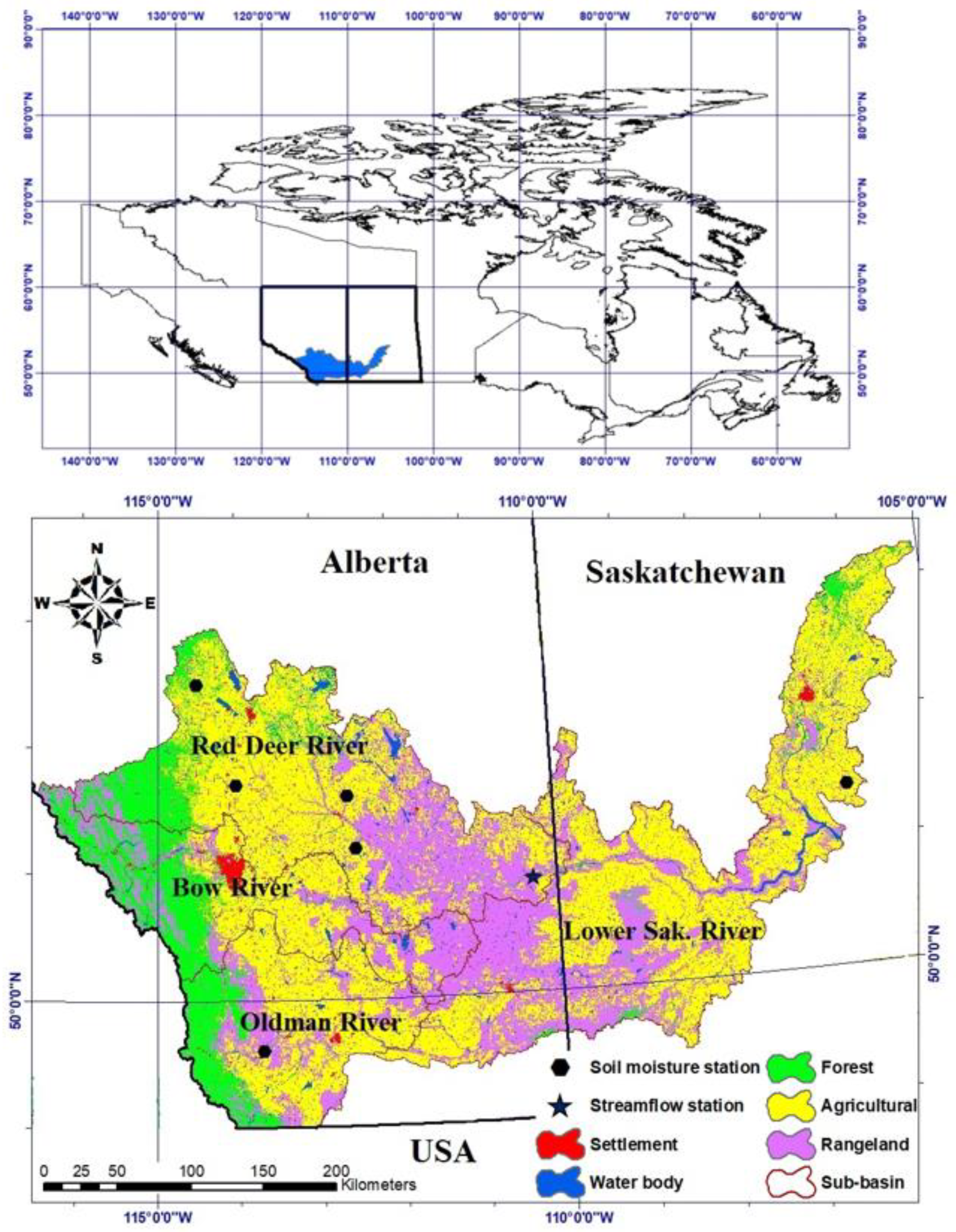
2.1. Study Area

SWC, soil temperature, and streamflow were evaluated in the SSRB (Figure 1). This region spans two provinces, Alberta and Saskatchewan, with an overall drainage area of 168,000 ${\mathrm{km}}^2$. The population of the SSRB is approximately 2.2 million; around 65% of the population is concentrated in Calgary and Saskatoon. The major sub-basins are the Red Deer River (RDR), Bow River (BR), Oldman River (OR), and Lower SSR (LSSR) [26]. The SSRB is characterized by a semi-arid continental climate with cold, dry winters and hot, humid summers. Precipitation is low due to the location of the SSRB on the leeward side of the Rocky Mountains [27]. Moreover, 80% of the annual runoff is generated by snowmelt during spring (March to April) and rainfall during summer (May to July). In summer, most of the rainfall infiltrates into the ground and evaporates from land and water surfaces and, as such, the rainfall contributes little to the overland runoff [28]. The average annual temperature ranges from 14 °C to 16 °C in summer and −2.5 to −8 °C in winter [29].

2.2. Data Description

Table 1. Input data used in SWAT model.

Data Type	Description	Information	Source
Digital Elevation Model	Watershed delineation	Raster, 30 m-resolution	Digital Elevation Model
			accessed on 24 August 2021
Land use	Land-use classification	Raster, 30 m-resolution	http://geogratis.gc.ca
			accessed on 30 August 2021
Soil type	Soil properties	Vector	http://www.agr.gc.ca
			accessed on 2 September 2021
Weather	Precipitation and temperature	Daily	https://weather.gc.ca
			accessed on 15 September 2021
Streamflow measured	Calibration and validation	Monthly	https://wateroffice.ec.gc.ca
			accessed on 4 December 2021
Soil Moisture measured	Calibration model	Daily	https://acis.alberta.ca
			accessed on 18 December 2021
Soil temperature	Calibration model	Daily	https://acis.alberta.ca
			accessed on 18 December 2021

summarizes the data used for hydrological modelling in the Arc SWAT interface. The SSRB was divided into 27 sub-basins using a 30-m resolution digital elevation model (DEM). Land use data for 2015 from Agriculture and Agri-Food Canada (AAFC) and soil data (Soil Landscapes of Canada, SLC ver. 3.2) were used for spatial discretization and modified to meet the input requirements of SWAT. Likewise, daily weather data from 1991 to 2020 were obtained for 15 stations from Environment and Climate Change Canada (ECCC). Daily stream discharge data for calibration (1993–2005) and validation (2006–2013) were obtained from the Water Survey of Canada (WSC) hydrometric database (HYDAT).

3. Methodology

In the SWAT model, a catchment or basin is integrated by delineating sub-basins based on inputs of land use, soil type and slope, which are then discretized into hydrologic response units (HRUs). The hydrologic component of SWAT is based on the water balance Equation (1) [2]:

$$S{W}_t=S{W}_o+{\displaystyle \sum }_{i=1}^t{(R_{day}-Q_{surf}-E_a-W_{seep}-Q_{gw})}_i$$

(1)

where $S{W}_t$ is the final soil water content (mm), $S{W}_o$ is the initial soil water content in day i (mm), t is the time (days), $R_{day}$ is the precipitation on day i (mm), $E_a$ is the evapotranspiration on day i (mm water), $W_{seep}$ is the amount of water entering the vadose zone from the soil profile on day i (mm), and $Q_{gw}$ is the return flow on day i (mm). A total of 4873 HRUs were delineated by defining a 2% level threshold for land use, a 5% level threshold for soil type, and a uniform slope to minimize the computational time. Six soil moisture monitoring stations from the Agricultural Drought Monitoring Network (AGDM) network are located in Alberta (Hussar AGDM, Morrin AGDM, Olds College AGDM, Leedale AGDM and Brocket AGDM). Another one is located in Saskatchewan (Kenaston). The data are recorded using the ML2X ThetaProbe soil moisture sensors from Delta-TDevice Ltd., Burwell, UK, which measure volumetric soil moisture content (θv) by responding to changes in the apparent dielectric constant, proportional to SWC. The soil temperature sensors are 107 probes manufactured by Campbell Scientific Inc. [30]. The snowmelt module in the SWAT model is divided into snow cover and snowmelt. We used the following mass balance equation at the HRU scale to monitor the snowpack for day i [31]:

$$SN{O}_i=SN{O}_{i-1}+S{F}_i-E_{subi}-SN{O}_{mlt}$$

(2)

where, for a given day i, $SN{O}_i$ and $SN{O}_{i-1}$ are the water content of the snowpack at the end of the day and the previous day ($\mathrm{mm} {\mathrm{H}}_2\mathrm{O}$), $S{F}_i$ is the total amount of snowfall ($\mathrm{m}\mathrm{m} {\mathrm{H}}_2\mathrm{O}$), $E_{subi}$ is the amount of sublimation ($\mathrm{m}\mathrm{m} {\mathrm{H}}_2\mathrm{O}$), and $SN{O}_{mlt}$ is the amount of snowmelt ($\mathrm{m}\mathrm{m} {\mathrm{H}}_2\mathrm{O}$). The timing of the onset of snowmelt is obtained using the degree-day factor method (as a sine function over time), which sets a snow-melting temperature threshold. The formula for the snowmelt calculation is as follows [19]:

$$SN{O}_{mlti}=b_{mlti}\times SN{O}_{covi}\left(\frac{T_{snow}+T_{maxi}}{2}-SMTMP\right)$$

(3)

The minimum and maximum values for a snow melt factor occur at the winter and summer solstices, respectively:

$$b_{mlti}=\frac{SMFMX+SMFMN}{2}+\frac{SMFMX-SMFMN}{2}\times \sin \left[\frac{2\pi }{365}\left(i-81\right)\right]$$

(4)

where $SMFMX$ and $SMFMN$ are the maximum and minimum snowmelt factors on 21 June and 21 December, respectively (mm H₂O·°C⁻¹·d⁻¹) and $i$ is the order of days in the calendar year.

As the initial condition of snow melting, the snowpack temperature is an average temperature of the previous day and varies as a dampened function of air temperature. The snowpack temperature is calculated as follows [31]:

$$T_{snow,t}=T_{snow,t-1}\times \left(1-TIMP\right)+T_a\times TIMP$$

(5)

where $T_{snow,t}$ is the snowpack temperature on a given day (°C), $T_{snow,t-1}$ is the snowpack temperature on the previous day (°C), $T_a$ is the average air temperature on that given day (°C) and $TIMP$ is the temperature lag factor. ROS is a common event in the SSRB. Rain falls on an existing snowpack, particularly at higher elevations in the headwaters of the SSRB. Therefore, hydrological models that do not employ ROS melt could have high errors when simulating streamflow and soil moisture. Hence, the SWAT model was modified using a snowmelt routine to include ROS melt using an energy balance equation based on a module written by Myers et al. [24]. For snowmelt during a ROS time interval ($m{m}_r, mm)$, the Equation (6) is:

$$\begin{array}{c}{M}_r=\sigma \times \Delta t_p\times (\left(T_a+273{)}^4-{273}^4\right)+0.0125\times P\times f_r\times T_r+8.5\times UADJ\times \frac{\Delta t_p}{6}\times (\left(0.9\times e_{sat}-6.11\right)\\ +0.00057\times P_a\times T_a)\end{array}$$

(6)

where $M_r$ is snow melt (mm), $\sigma$ is the ROS melt rate per temperature degree over time from radiative heat transfer ($-6.12\times {10}^{-10}\mathrm{mm}/\mathrm{K}/\mathrm{h}$; [32]); $\Delta t_p$ is the time interval of precipitation, $T_a$ is air temperature ($℃)$, $P_a$ is total precipitation and snowfall (mm/h), $f_r$ is the fraction of precipitation in the form of rain, $T_r$ is rain temperature (max of $T_a$ or 0 $℃$), $UADJ$ represents the influence of wind on ROS melt (mm/mb/6 h), $e_{sat}$ is saturation vapour pressure (mb), and $P_a$ is atmospheric pressure (mb). Moreover, $e_{sat}$ is computed from:

$$e_{sat}=2.7489\times {10}^8\times e{ }^{\frac{-4278.63}{T_{}}}$$

(7)

$$P_a=33.86(29.9-0.335H_e)+0.00022H_{e^{2.4}}$$

(8)

where $H_e$ is sub-basin elevation (m).

Soil temperature is a function of the surface temperature, mean annual air temperature and the depth of soil in the SWAT model. Soil temperature in the SWAT model is calculated for each HRU at the center of the soil layer. The formula is as follows [1]:

$$T_{soil}\left(z,d_n\right)=\gamma .T_{soil}\left(z,d_n-1\right)+\left[1-\gamma \right].\left[df.\left({\overline{T}}_{Aair}-T_{sur}\right)+T_{sur}\right]$$

(9)

where $T_{soil}\left(z,d_n\right)$ is the soil temperature (°C) at depth $z$ (mm) and day of the year $d_n$, $\gamma$ is the lag coefficient controlling the influence of previous day’s temperature on the current day’s temperature (ranging from 0 to 1), $T_{soil}\left(z,d_n-1\right)$ is the soil temperature (°C) at depth z from the previous day, $df$ is the depth factor that quantifies the influence of depth below the surface on soil temperature, ${\overline{T}}_{Aair}$ is the average annual air temperature (°C), and $T_{sur}$ is the soil surface temperature on the day. One of the drawbacks to using this empirical formula is that it is unable to simulate freeze-thaw cycles as phase changes are not considered in the SWAT model and were found severely underestimated in the winter season [1,23]. Therefore, we used a physically based soil temperature module developed by Qi et al. [23].

Yin and Arp [33] describe heat transfer in snow and soil layers by assuming that temperature changes are governed by heat conduction through the soil layers and latent heat exchange, originating from freeze-thaw cycles in the upper soil profile:

$$\frac{\partial T}{\partial t}=\frac{\partial }{\partial x}\left(\frac{k}{c}.\frac{\partial T}{\partial x}\right)\frac{s}{c}$$

(10)

where $T$ is the temperature (°C), $t$ is the time step (in days, d), $k$ is the thermal conductivity (${\mathrm{J} \mathrm{cm}}^{-1}{\mathrm{d}}^{-1}{℃}^{-1})$, $c$ is the volumetric heat capacity (${\mathrm{J} \mathrm{cm}}^{-3}{℃}^{-1})$, $x$ is the vertical distance from the air-soil or air-snow interface (cm), and $s$ represents the latent heat sink term (${\mathrm{J} \mathrm{cm}}^{-1}{\mathrm{d}}^{-1}{℃}^{-1})$.

The SWAT model simulates soil temperature per layer in the center of an HRU. The enhanced version of SWAT, with the physically-based representation of freeze-thaw cycles, has been employed to simulate soil temperature, soil thermal conditions, and freeze-thaw cycles in both small and large watersheds in North America [1,23,34,35,36]. The major difference between the SWAT-B and SWAT-M models is implementing a combination of the physically-based soil temperature module, instead of an empirical module, with an energy budget equation for snowmelt during a ROS event.

The SWC component in the SWAT model consists of soil structure elements that determine the permanent wilting point volumetric water content as a function of the clay content and bulk density. Wilting point was estimated in the SWAT model for each soil layer as Equation (11) [2]:

$$W{P}_{ly}=0.4\frac{m_c\times {\rho }_b}{100}$$

(11)

where $W{P}_{ly}$ is the water content at wilting point, $m_c$ is the clay content of the soil layer (%), and ${\rho }_b$ is the bulk density for the soil layer ($\mathrm{M}\mathrm{g}{\mathrm{m}}^{-3}$). Field capacity water content is estimated as per the following Equation (12):

$$F{C}_{ly}=W{P}_{ly}+AW{C}_{ly}$$

(12)

where $F{C}_{ly}$ is the water content at field capacity expressed as a fraction of the total soil volume, $W{P}_{ly}$ is the water content at the wilting point, and $AW{C}_{ly}$ is the available water capacity of the soil layer. Water in excess of the field capacity is available for infiltration and lateral flow except when the soil layer is frozen. In this study, we considered SWC in the warm season of April to September.

The SWAT-CUP and the Sequential Uncertainty Fitting (SUFI-2) program [37] were used for the sensitivity, calibration, and uncertainty analyses of the model runs. The SUFI-2 was applied to data for calibration and validation, with two iterations of 500 simulations. A one-factor-at-a-time (LH-OAT) and global sensitivity analysis procedure are embedded in the SWAT model. The resulting sensitive parameters were calibrated against the observed runoff data from the outlet streamflow stations [38]. During calibration and validation, SWAT model performance was evaluated through a graphical comparison of the simulated and observed monthly streamflow hydrographs and three statistical criteria for goodness-of-fit: the Nash-Sutcliffe efficiency (NSE) [39], the percent bias (PBIAS) [40], and the coefficient of correlation ($r$) [41] as follows (Equations (13)–(15)):

$$NSE=\left[1-\frac{{{\displaystyle \sum }}_{i=1}^n{\left(Q_i^{obs}-{\overline{Q}}_i^{sim}\right)}^2}{{{\displaystyle \sum }}_{i=1}^n{\left(Q_i^{obs}-Q_{mean}^{obs}\right)}^2{}^{}}\right]$$

(13)

$$PBIAS=\frac{{{\displaystyle \sum }}_{i=1}^n{\left(Q_i^{obs}-Q_i^{sim}\right)}^{}}{{{\displaystyle \sum }}_{i=1}^n{Q}_i^{obs}{}^{}}\times 100$$

(14)

$$r=\frac{{{\displaystyle \sum }}_{i=1}^n\left(Q_i^{obs}-{\overline{Q}}_i^{obs}\right).{\left(Q_i^{sim}-{\overline{Q}}_i^{sim}\right)}^{}}{\sqrt{{{\displaystyle \sum }}_{i=1}^n(}{Q}_i^{obs}-{\overline{Q}}_i^{obs}{)}^2.\sqrt{{{\displaystyle \sum }}_{i=1}^n{(Q_i^{sim}-{\overline{Q}}_i^{sim})}^2}}$$

(15)

where, ${\overline{Q}}_i^{sim}$ and ${\overline{Q}}_i^{obs}$ are the mean monthly simulated and observed discharge, $Q_i^{obs}$ is observed discharge on the ith day, $Q_i^{sim}$ is the simulated monthly discharge, n is the total number of months, and $Q_{mean}^{obs}$ is the average observed monthly streamflow. The statistical measures of these uncertainties are the P-factor (observation data in the 95% prediction uncertainty, 95PPU) and the R-factor (ratio of average width of the 95PPU band to the standard deviation of the measured data). These two factors collectively capture most of the measured data with the smallest possible uncertainty band. The best fit for calibration and prediction uncertainty is 100% for p factor and 1 for r factor. We employed multivariable calibration of monthly streamflow at the watershed outlet and of daily SWC and soil temperature at the location of the field sensors in the associated HRU (Figure 1). Given relatively long streamflow records, we were able to validate the simulation of streamflow. Validation of SWC and soil temperature was not possible, however, because the observational data were limited to five years.

4. Results

4.1. Model Sensitivity Analysis

Table 2. Performance indices of SWAT-M parameters in the SSRB.

Parameter	Range	SWAT-M				SWAT-B			Fitted Value
		Rank	p-Value	t-State	Fitted Value	Rank	p-Value	t-State
CN2	−0.2–0.2	1	0.00	7.96	0.15	1	0.00	8.32	0.18
SOL_AWC	−0.1–1.0	2	0.00	5.3	0.35	9	0.61	−0.5	−0.075
SFTMP	−5–5	3	0.01	−2.33	3.52	3	0.24	1.17	2.68
SMFMN	0–10	4	0.03	−2.09	7.42	-	-	-	-
SOL_BD	−0.1–1.0	5	0.11	−1.56	0.23	6	0.41	0.81	0.26
SOL_K	−0.1–1.0	6	0.21	1.24	0.62	5	0.29	1.04	0.62
SOL_Z	−0.1–1.0	7	0.21	−1.23	−0.05	-	-	-	-
SMTMP	−5–5	8	0.38	0.87	−4.22	12	0.84	0.19	−2.49
GWQMN	0–2	9	0.56	0.58	0.24	7	0.5	0.66	0.23
SMFMX	0–10	10	0.58	0.54	0.52	2	0.1	1.64	1.83
CH_K2	0–500	11	0.61	0.49	387	8	0.58	0.54	391
SURLAG	0–24	12	0.71	−0.36	8.33	-	-	-	-
CH_N2	0–0.3	13	0.71	−0.36	0.03	13	0.88	0.14	0.017
ESCO	0.0–1.0	14	0.8	−0.24	0.44	4	0.13	1.12	0.81
ALPHA_BF	0.0–1.0	15	0.84	0.2	0.55	10	0.71	0.36	0.52
GW_DELAY	−0.2–0.2	16	0.89	0.13	0.18	11	0.78	0.22	0.17
SUB_SMFMN	0.0–10	17	0.9	−0.12	0.63	-	-	-	-
SOL_ALB	0.0–0.25	18	0.92	0.09	0.07	14	0.96	0.04	0.07

shows the results of sensitivity analysis with the SUFI-2 method for a period of 19 years for the base and modified SWAT models. They indicate the 18 and 14 most sensitive parameters (SWAT-M and SWAT-B, respectively) for streamflow, SWC, and snowmelt simulation in the SSRB among the 30 input parameters. The t-statistic represents the degree of sensitivity (larger values are more sensitive), and p-values indicate the significance of the sensitivity (closer to zero are more significant). After modifying the SWAT model, the most sensitive parameters were curve number at moisture condition (CN2) followed by soil water content (SOL_AWC). CN2 was the most sensitive parameter in similar studies [42,43,44,45]. Four snowmelt-related parameters ranked among the ten most sensitive parameters, including snowfall temperature (°C), the snowmelt base temperature (SMTMP), and the maximum and minimum temperature-index snowmelt factors (SMFMX and SMFMN). This finding is similar to Liu et al. [46]. Generally, eight parameters with p < 0.5 were found to have the most significant effect on streamflow, soil moisture and snowmelt, and therefore, they contributed the least to model uncertainties at the catchment scale.

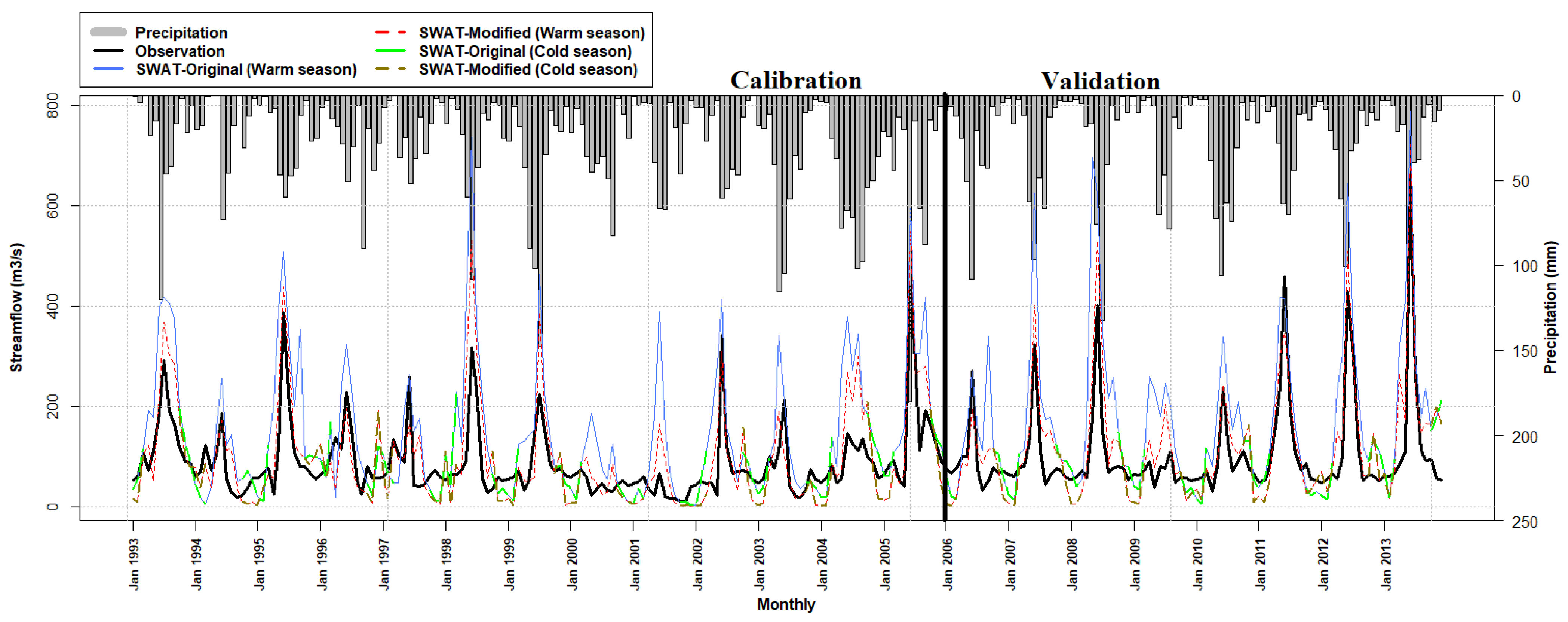
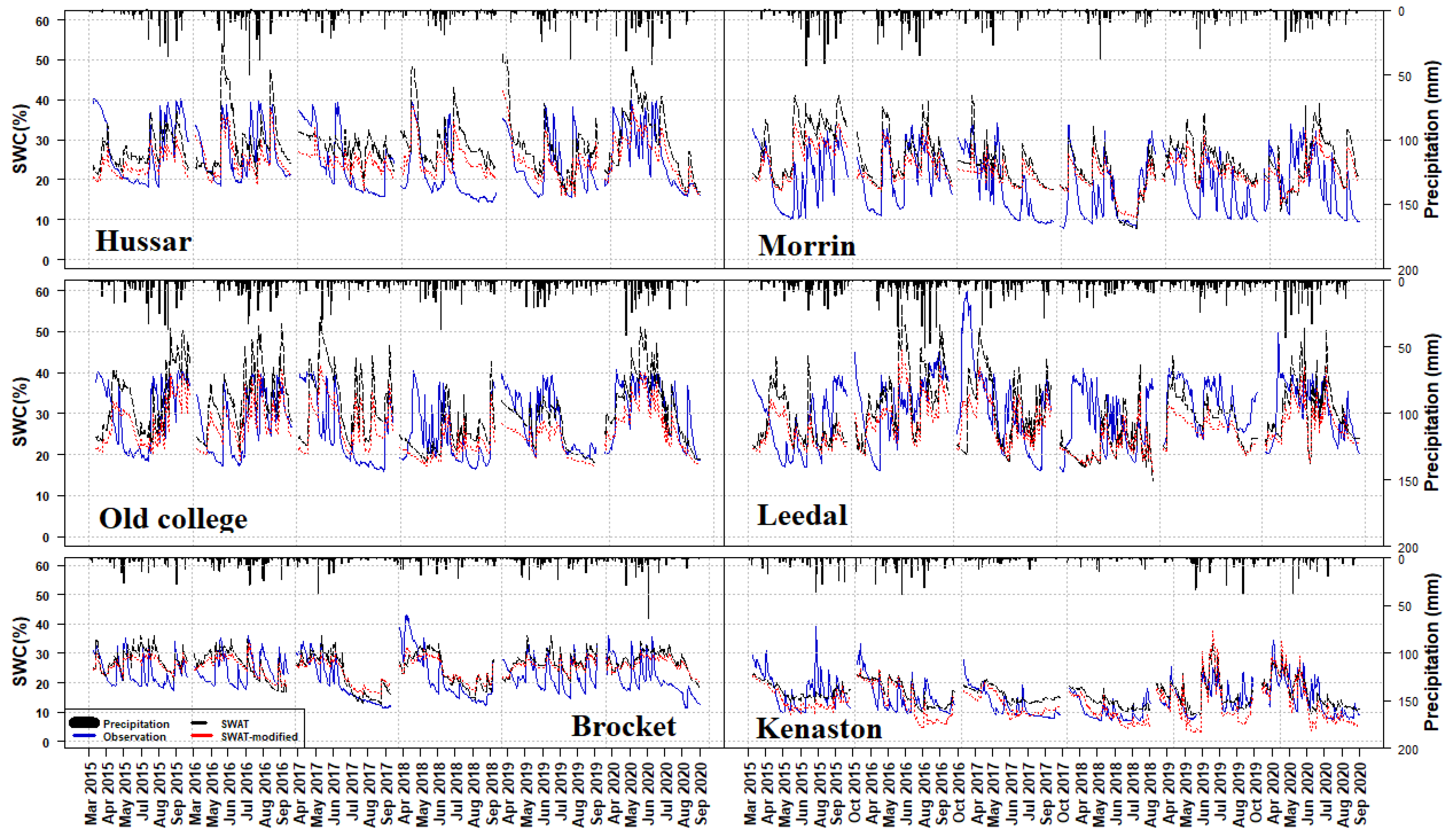
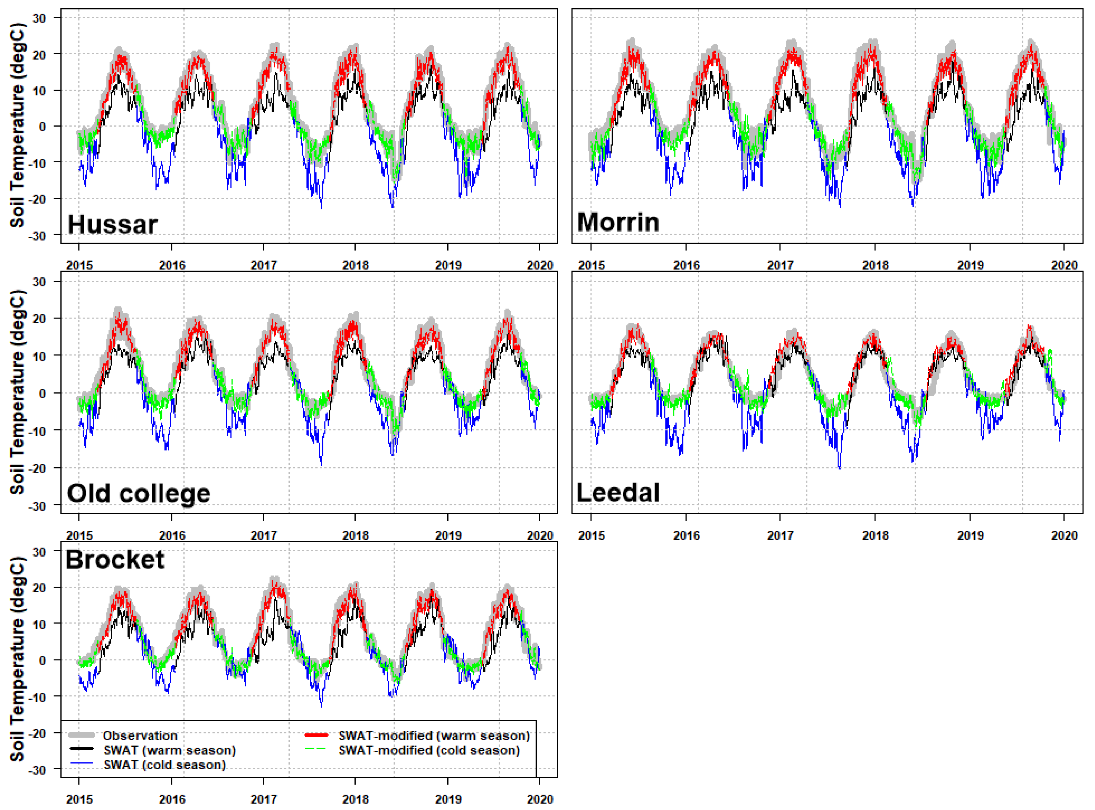
4.2. Calibration and Validation

Table 3. Monthly calibration and validation of SWAT-B and SWAT-M SWAT.

Statistics	Calibration (1993–2005)		Validation (2006–2013)
	SWAT-B	SWAT-M	SWAT-B	SWAT-M
$NSE$	0.39	0.71	0.42	0.76
$PBIAS$	−18.3	−9.3	−19.2	−8.4
$r$	0.72	0.83	0.75	0.88

gives the statistical output from the calibration and validation of the base and modified SWAT models. The results reveal NSE values between 0.39 and 0.76. A NSE greater than 0.5 indicates that the SWAT-M performance is satisfactory at the monthly time step [47]. Similarly, r values confirm good correlation between observed and simulated streamflow in SWAT-M and acceptable correlation for SWAT-B. The PBIAS factor for the two periods shows very good performance ((PBIAS < ±10%) for SWAT-M and satisfactory (±15% ≤ PBIAS ≤ ±25%) for SWAT-B. Furthermore, SWAT-M exhibited a significant improvement in statistical indices.

Figure 2 gives calibration and validation results from SUFI-2 comparing observed and simulated streamflow from 1993 to 2005 and 2006 to 2013, respectively. The monthly mean of observed streamflow was 66.58 ${\mathrm{m}}^3·{\mathrm{s}}^{-1}$ during the non-melting period (October-March), while the simulated streamflow for SWAT-B and SWAT-M was 89 and 54.22 ${\mathrm{m}}^3·{\mathrm{s}}^{-1}$, respectively. The simulation of streamflow showed an overestimate before model improvement during the cold season, which was reduced after modifying the SWAT. During the warm season (April-September), the observed monthly average streamflow was 122.86 ${\mathrm{m}}^3·{\mathrm{s}}^{-1}$ while the simulated streamflow for SWAT-B and SWAT-M was 239.12 and 159.6 ${\mathrm{m}}^3·{\mathrm{s}}^{-1}$, respectively. These results confirm that the modified SWAT model improves streamflow simulation relative to the actual measured values. Furthermore, the peak value of the SWAT-M declined compared with the SWAT-B simulation, mainly after the snowmelt period, and modified values are closer to observed values. According to Zare et al. (2022), the SWAT model tends to underestimate runoff in the early spring (April and May) due to uncertainties in input data and model structure for snowmelt and runoff season. This has been significantly adjusted here by modifying the source code.

Table 4. Daily statistical analysis between SWAT-B and SWAT-M with measurement data for SWC and soil temperature (ST).

	Statistical Indices	$\mathit{r}$		PBIAS		NSE
	Station	SWAT-B	SWAT-M	SWAT-B	SWAT-M	SWAT-B	SWAT-M
SWC	Hussar	0.48	0.55	−13.6	9.5	0.61	0.72
	Morrin	0.52	0.53	−22	−10.2	0.67	0.79
	Olds College	0.45	0.45	14	−9.1	0.49	0.61
	Leedale	0.24	0.33	16.6	15.7	0.46	0.57
	Brocket	0.5	0.57	−13.1	−8.2	0.74	0.86
	Kenaston	0.6	0.65	−11	7.1	0.64	0.78
	Mean	0.47	0.51	15.5	10	0.60	0.72
ST	Hussar	0.92	0.9	6.5	2.8	0.32	0.6
	Morrin	0.91	0.9	6.8	3.09	0.32	0.67
	Olds College	0.9	0.9	4.7	1.95	0.48	0.74
	Leedale	0.88	0.88	3.3	1.2	0.61	0.74
	Brocket	0.87	0.87	4	3.8	0.37	0.71
	Mean	0.90	0.9	5.06	2.57	0.42	0.69

summarizes the statistical performance of the SWAT-B and SWAT-M models for the warm season based on daily measurement data and three error metrics (i.e., NSE, PBIAS, and $r$). The average of PBIAS indices for all stations revealed that the SWAT-B model performance was satisfactory ($\pm 15\%\le PBIAS\le \pm 25\%)$ to simulate SWC, however, this measure is much improved for SWAT-M ($\pm 10\%\le PBIAS\le \pm 15\%)$. In all stations, calibration results showed a satisfactory fit between simulated and measured SWC. SWAT-M exhibited a significant improvement in statistical indices for all stations so that the NSE and PBIAS changed from satisfactory to good fit at some stations (Brocket, Hussar, and Kenaston). Similarly, we compared daily soil temperature from the two SWAT models to observed values. The average r values among all stations are statistically significant (p < 0.05), while SWAT-M has better results in terms of PBIAS and NSE. However, both models provide very good soil temperature estimation.

Figure 3 depicts a daily time series (warm season) of simulated SWC (SWAT-B and SWAT-M) and observations during the calibration period. The agreement validates the ability of the SWAT to model SWC. The measured data are a better fit with SWAT-M compared with SWAT-B output. SWAT-B values are higher than SWAT-M output and field measurements, while the range of SWAT-M has become a much better fit with observations.

Figure 4 shows observed, SWAT-B, and SWAT-M soil temperatures for the five stations. The results indicate that SWAT-B tends to underestimate soil temperature in the cold season while SWAT-M significantly improved soil temperature simulation for winter. The lowest simulated soil temperature by the SWAT-B model was −20 $℃$, whereas the soil temperature simulated by the SWAT-M was −3.5 $℃$ and was close to the observations in the cold season. However, both SWAT versions simulated soil temperature that were slightly less than observations in the warm season.

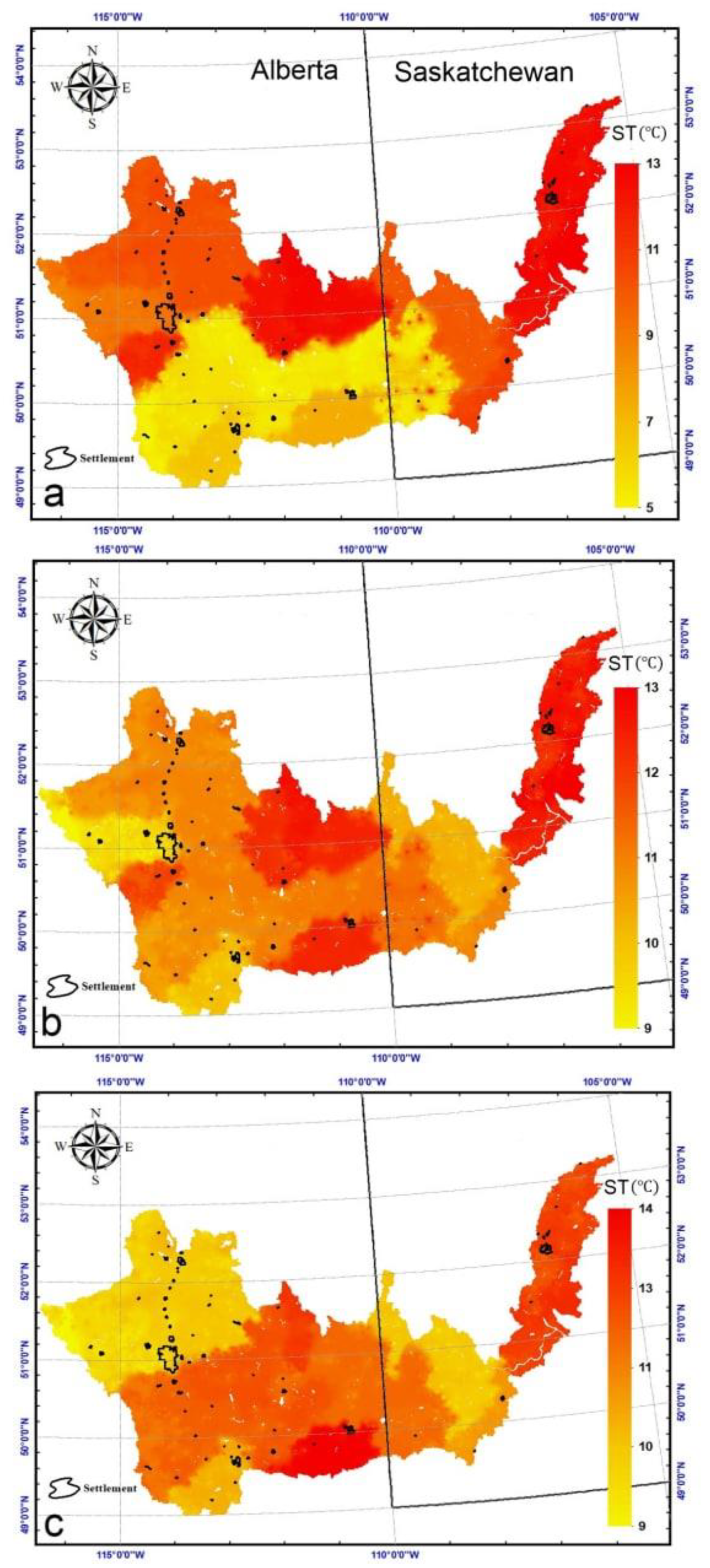
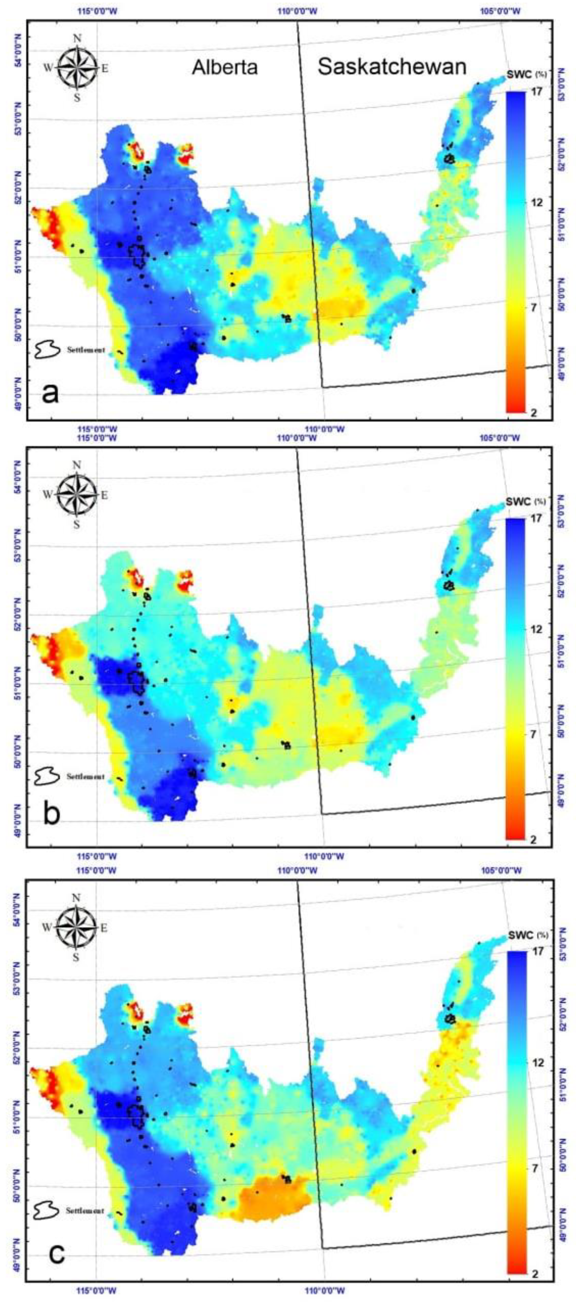
4.3. Spatial Pattern of SWC and Soil Temperature

Figure 5 and Figure 6 show the spatial-temporal patterns of soil temperature and warm-season SWC during three successive decades: 1991–2000, 2001–2010, and 2011–2020. The spatial distributions are similar for all decades; however, the temporal variations of soil temperature and SWC are different. The average SWC among all HRUs was 12.8, 10.6, and 10.9% from the first decade to the third decade. Mean soil temperature for all HRUs was 9.5, 11.8, and 11.4 °C from the first decade to the third decade. Generally, the lowest SWC appeared in the Rocky Mountains (the western SSRB), whereas high SWC was observed in the southern area, particularly nearby Lethbridge for all decades. Moreover, there are apparent changing trends from the first to the third decade in the east and south, which become much drier. The highest soil temperature was from Swift Current to Saskatoon for all decades, and the lowest soil temperature was in the center of the basin and to the south in the first decade, although it increased in the last decade. The eastern part of the SSRB is much drier than the higher elevations to the west [12,48].

5. Discussion

The SWAT-M module is able to simulate freeze-thaw cycles and capture the impact of snow cover on frozen water content variation in the surface soil. For this reason, it overcomes the drawback of the SWAT-B for the simulation of streamflow and soil temperature in the cold season, as reported by some researchers [2,23,49]. The SWAT-M subroutine simulated soil temperature and SWC that compare very well with observational data in the cold region SSRB of western Canada. The module gave better results for soil temperature and streamflow, although slightly underestimating soil temperature and particularly SWC in the warm season. This might be attributed to the uncertainty in soil properties, including density, texture, permeability, and organics, all of which affect the range of expected soil moisture variations. This finding is similar to Qi et al. [50], having underestimated SWC due to uncertainty in soil data. Assimilating remote sensing data, such as SMAP, and field data could overcome this problem. Furthermore, a good fit among SWC simulations was observed in the farming season (from May to September); the best correlation occurred when vegetation reached the peak growth rate. Crops play a significant role in the surface energy balance, affecting soil temperature and moisture via their interaction with convective heat transfer [51,52]. One of the soil physical parameters that can be adjusted is soil thermal conductivity coefficient $k_{coe}$. This parameter is assigned a value of one (=1) in the SWAT model. Qi et al. [2] recommended that the value of $k_{coe}$ should be changed based on humidity and surface cover. The results showed a better simulation when this value was less than the default. It better addressed crop residue in the surface layers in the warm season, particularly the growing season; statistical analysis showed a great disparity between soil moisture stations. In addition, we employed multivariable calibration via evaluation of monthly streamflow along with daily SWC and soil temperature. This improved the reliability of parameters for simulating the hydrology of the SSRB. Another advantage of the SWAT-M, which combined an energy balance snowmelt equation with physically-based soil temperature, was incorporating freeze-thaw cycles into SWAT source code with no additional input data or setup requirements.

6. Conclusions

A new algorithm was employed to calibrate SWC and soil temperature for the snowmelt simulation in the SWAT model. These results confirm that the SWAT-M model improves streamflow simulation relative to the actual measured values with PBIAS less than 10% and NSE and R higher than 0.7. Furthermore, the SWAT-M model provides a better simulation of SWC, that is, a better fit between modelled and measured data. SWAT-B values are higher than SWAT-M output and field measurements, while the range of SWAT-M output has a much better fit with observed SWC. Furthermore, the results of soil temperature showed an improved simulation of this parameter by SWAT-M, particularly for the cold season. This new SWAT module simulates freeze-thaw cycles and captures the influence of snow cover on soil surface ice-water content. Thus, we overcame the drawback of the SWAT model for the simulation of streamflow and soil temperature in the cold season. Spatial analysis of SWC and soil temperature showed that the SWAT-M predicted more SWC and lower soil temperature in the western SSRB, while higher soil temperature along with low SWC in the eastern part of the basin. SWC and soil temperature from SWAT-M indicate that recently (2011–2020) conditions are drier across almost the whole region than in the preceding decade (1991–2000). Soil moisture plays a vital role in dryland agriculture, which relies on rain and snowmelt. Low SWC and high soil temperature in the warm season are problematic for the production of dryland crops. These conditions will intensify in the presence of climate change.

References

1. Qi, J.; Zhang, X.; Cosh, M.H. Modeling soil temperature in a temperate region: A comparison between empirical and physically based methods in SWAT. Ecol. Eng. 2019, 129, 134–143. [Google Scholar] [CrossRef]
2. Zare, M.; Azam, S.; Sauchyn, D. Evaluation of Soil Water Content Using SWAT for Southern Saskatchewan, Canada. Water 2022, 14, 249. [Google Scholar] [CrossRef]
3. Park, J.Y.; Ahn, S.R.; Hwang, S.J.; Jang, C.H.; Park, G.A.; Kim, S.J. Evaluation of MODIS NDVI and LST for indicating soil moisture of forest areas based on SWAT modeling. Pad. Water Environ. Eng. 2014, 121, 77–88. [Google Scholar] [CrossRef]
4. Yang, Y.T.; Roderick, M.L.; Zhang, S.L.; McVicar, T.R.; Donohue, R.J. Hydrologic implications of vegetation response to elevated CO2 in climate projections. Nat. Clim. Chang. 2019, 9, 44–49. [Google Scholar] [CrossRef]
5. Koerselman, W.; Van Kerkhoven, M.B.; Verhoeven, J.T. Release of inorganic N, P and K in peat soils; effect of temperature, water chemistry and water level. Biogeochemistry 1993, 20, 63–81. [Google Scholar] [CrossRef]
6. Stoller, E.W.; Wax, L.M. Temperature variations in the surface layers of an agricultural soil. Weed Res. 1973, 13, 273–282. [Google Scholar] [CrossRef]
7. Wheater, H.S.; Gober, P.A. Water security in the Canadian Prairies: Science and management challenges. Philos. Trans. R. Soc. 2013, 371, 20120409. [Google Scholar] [CrossRef]
8. Chipanshi, A.C.; Findlater, K.M.; Hadwen, T.; O’Brien, E.G. Analysis of consecutive droughts on the Canadian prairies. Clim. Res. 2006, 30, 175–187. [Google Scholar] [CrossRef]
9. Bonsal, B.R.; Wheaton, E.E.; Chipanshi, A.C.; Lin, C.; Sauchyn, D.J.; Wen, L. Drought research in Canada: A review. Atmos. Ocean 2011, 49, 303–319. [Google Scholar] [CrossRef]
10. Sauchyn, D.; Ilich, N. Nine Hundred Years of Weekly Streamflows: Stochastic Downscaling of Ensemble Tree-Ring Reconstructions. Water Resour. Res. 2017, 53, 9266–9283. [Google Scholar] [CrossRef] [Green Version]
11. Bonsal, B.; Aider, R.; Gachon, P.; Lapp, S. An assessment of Canadian prairie drought: Past, present, and future. Clim. Dyn. 2013, 41, 501–516. [Google Scholar] [CrossRef]
12. Masud, M.B.; Khaliq, M.N.; Wheater, H.S. Analysis of meteorological droughts for the Saskatchewan River basin using univariate and bivariate approaches. J. Hydrol. 2015, 522, 452–466. [Google Scholar] [CrossRef]
13. Arnold, J.G.; Moriasi, D.N.; Gassman, P.W.; Abbaspour, K.C.; White, M.J.; Srinivasan, R.; Santhi, C.; Harmel, R.D.; Van Griensven, A.; Van Liew, M.W.; et al. SWAT: Model use, calibration, and validation, Trans. ASABE 2012, 55, 1491–1508. [Google Scholar] [CrossRef]
14. Yang, X.; Liu, Q.; He, Y.; Luo, X.; Zhang, X. Comparison of daily and sub-daily SWAT models for daily streamflow simulation in the Upper Huai River Basin of China. Stoch. Environ. Res. Risk Assess. 2016, 30, 959–972. [Google Scholar] [CrossRef]
15. Refsgaard, J.C.; Storm, B. MIKE-SHE. In Computer Models of Watershed Hydrology; Singh, V.J., Ed.; Water Resour Pub.: Englewood, CO, USA, 1995; pp. 809–846. [Google Scholar]
16. Mapfumo, E.; Chanasyk, D.S.; Willms, W.D. Simulating daily soil water under foothills fescue grazing with the Soil and Water Assessment Tool model (Alberta, Canada). Hydrol. Process. 2004, 18, 2787–2800. [Google Scholar] [CrossRef]
17. Narasimhan, B.; Srinivasan, R. Development and evaluation of Soil Moisture Deficit Index (SMDI) and Evapotranspiration Deficit Index (ETDI) for agricultural drought monitoring. Agric. For. Meteorol. 2005, 133, 69–88. [Google Scholar] [CrossRef]
18. Havrylenko, S.B.; Bodoque, J.M.; Srinivasan, R.; Zucarelli, G.V.; Mercuri, P. Assessment of the soil water content in the Pampas region using SWAT. Catena 2016, 137, 298–309. [Google Scholar] [CrossRef]
19. Lévesque, É.; Anctil, F.; Van Griensven, A.N.N.; Beauchamp, N. Evaluation of streamflow simulation by SWAT model for two small watersheds under snowmelt and rainfall. Hydrol. Sci. J. 2008, 53, 961–976. [Google Scholar] [CrossRef]
20. Grusson, Y.; Sun, X.; Gascoin, S.; Sauvage, S.; Raghavan, S.; Anctil, F.; Sanchez Pérez, J.M. Assessing thevcapability of the SWAT model to simulate snow, snow melt and streamflow dynamics over an alpinevwatershed. J. Hydrol. 2015, 531, 574–588. [Google Scholar] [CrossRef]
21. Masud, M.B.; McAllister, T.; Cordeiro, M.R.C.; Faramarzi, M. Modeling future water footprint of barley production in Alberta, Canada: Implications for water use and yields to 2064. Sci. Total Environ. 2018, 616, 208–222. [Google Scholar] [CrossRef]
22. Liang, K.; Jiang, Y.; Qi, J.; Fuller, K.; Nyiraneza, J.; Meng, F.R. Characterizing the impacts of land use on nitrate load and water yield in an agricultural watershed in Atlantic Canada. Sci. Total Environ. 2020, 729, 138793. [Google Scholar] [CrossRef] [PubMed]
23. Qi, J.; Li, S.; Li, Q.; Xing, Z.; Bourque, C.P.-A.; Meng, F.-R. A new soil-temperature module for swat application in regions with seasonal snow cover. J. Hydrol. 2016, 538, 863–877. [Google Scholar] [CrossRef]
24. Myers, D.T.; Ficklin, D.L.; Robeson, S.M. Incorporating rain-on-snow into the SWAT model results in more accurate simulations of hydrologic extremes. J. Hydrol. 2021, 603, 126972. [Google Scholar] [CrossRef]
25. Rücker, A.; Boss, S.; Kirchner, J.W.; von Freyberg, J. Monitoring snowpack outflow volumes and their isotopic composition to better understand streamflow generation during rain-on-snow events. Hydrol. Earth Syst. Sci. Discuss. 2019, 23, 2983–3005. [Google Scholar] [CrossRef]
26. Morales-Martín, L.; Wheater, H.; Lindenschmidt, K.E. Potential changes of annual averaged nutrient export in the South Saskatchewan River Basin under climate and land use change scenarios. Water 2018, 10, 1438. [Google Scholar] [CrossRef]
27. Tanzeeba, S.; Gan, T.Y. Potential impact of climate change on the water availability of South Saskatchewan River Basin. Clim. Chang. 2012, 112, 355–386. [Google Scholar] [CrossRef]
28. Pomeroy, J.; Fang, X.; Williams, B. Impacts of Climate Change on Saskatchewan’s Water Resources; Centre for Hydrology, University of Saskatchewan: Saskatoon, SK, Canada, 2009. [Google Scholar]
29. Lac, S. A Climate change adaptation study for the South Saskatchewan River Basin. In SSHRC MCRI-Institutional Adaptation to Climate Change Project; Canadian Plains Research Centre, University of Regina: Regina, SK, Canada, 2004. [Google Scholar]
30. Agboma, C.; Itenfisu, D. Investigating the Spatio-Temporal dynamics in the soil water storage in Alberta’s Agricultural region. J. Hydrol. 2020, 588, 125104. [Google Scholar] [CrossRef]
31. Neitsch, S.L.; Arnold, J.G.; Kiniry, J.R.; Williams, J.R. Soil and Water Assessment Tool–Theoretical Documentation Version 2009; Technical Report 406; Texas Water Resources Institute: Forney, TX, USA, 2011; 647p. [Google Scholar]
32. Anderson, E.E.; Viskanta, R. Spectra1 and boundary effects on coupled conduction. Radiation heat transfer through semi-transparent solids. Wiirme StojZibertragung 1973, 1, 14–24. [Google Scholar] [CrossRef]
33. Yin, X.; Arp, P.A. Predicting forest soil temperatures from monthly air temperature and precipitation records. Can. J. For. Res. 1993, 23, 2521–2536. [Google Scholar] [CrossRef]
34. Qi, J.Y.; Li, S.; Yang, Q.; Xing, Z.S.; Meng, F.R. SWAT Setup with Long-Term Detailed Landuse and Management Records and Modification for a Micro-Watershed Influenced by Freeze-Thaw Cycles. Water Resour. Manag. 2017, 31, 3953–3974. [Google Scholar] [CrossRef]
35. Wang, Q.; Qi, J.; Wu, H.; Zeng, Y.; Shui, W.; Zeng, J.; Zhang, X. Freeze-Thaw cycle representation alters response of watershed hydrology to future climate change. CATENA 2020, 195, 104767. [Google Scholar] [CrossRef]
36. Qi, J.; Zhang, X.; Wang, Q. Improving hydrological simulation in the Upper Mississippi River Basin through enhanced freeze-thaw cycle representation. J. Hydrol. 2019, 571, 605–618. [Google Scholar] [CrossRef]
37. Abbaspour, K.C.; Yang, J.; Maximov, I.; Siber, R.; Bogner, K.; Mieleitner, J.; Zobrist, J.; Srinivasan, R. Modelling hydrology and water quality in the pre-alpine/alpine Thur watershed using SWAT. J. Hydrol. 2007, 333, 413–430. [Google Scholar] [CrossRef]
38. Van Griensven, A.; Meixner, T.; Grunwald, S.; Bishop, T.; Di Luzio, M.; Srinivasan, R. A global sensitivity analysis method for the parameters of multi-variable watershed models. J. Hydrol. 2006, 324, 10–23. [Google Scholar] [CrossRef]
39. Nash, J.E.; Sutcliffe, J.V. River flow forecasting through conceptual models: Part I—A discussion of principles. J. Hydrol. 1970, 10, 282–290. [Google Scholar] [CrossRef]
40. Moriasi, D.N.; Arnold, J.G.; Van Liew, M.W.; Binger, R.L.; Harmel, R.D.; Veith, T. Model evaluation guidelines for systematic quantification of accuracy in watershed simulations. Trans. ASABE 2007, 50, 885–900. [Google Scholar] [CrossRef]
41. Legates, D.R.; McCabe, G.J. Evaluating the use of “goodness-of-fit” measures in hydrological and hydroclimatic model validation. Water Resour. Res. 1999, 35, 233–241. [Google Scholar] [CrossRef]
42. Mamo, K.H.M.; Jain, M.K. Runoff and sediment modeling using SWAT in Gumera catchment, Ethiopia. Open J. Mod. Hydrol. 2013, 2013. [Google Scholar] [CrossRef]
43. Gyamfi, C.; Ndambuki, J.M.; Salim, R.W. A historical analysis of rainfall trend in the Olifants Basin in South Africa. Earth Sci. Res. 2016, 5, 129–142. [Google Scholar] [CrossRef]
44. Khalid, K.; Ali, M.F.; Rahman, N.F.A.; Mispan, M.R.; Haron, S.H.; Othman, Z.; Bachok, M.F. Sensitivity analysis in watershed model using SUFI-2 algorithm. Procedia Eng. 2016, 162, 441–447. [Google Scholar] [CrossRef] [Green Version]
45. Thavhana, M.P.; Savage, M.J.; Moeletsi, M.E. SWAT model uncertainty analysis, calibration and validation for runo ff simulation in the Luvuvhu River catchment, South Africa. Phys. Chem. Earth 2018, 105, 115–124. [Google Scholar]
46. Liu, Y.; Cui, G.; Li, H. Optimization and Application of Snow Melting Modules in SWAT Model for the Alpine Regions of Northern China. Water 2020, 12, 636. [Google Scholar] [CrossRef]
47. Moriasi, D.N.; Gitau, M.W.; Pai, N.; Daggupati, P. Hydrologic and water quality models: Performance measures and evaluation criteria. Trans. ASABE 2015, 58, 1763–1785. [Google Scholar]
48. Islam, Z.; Gan, T.Y. Potential combined hydrologic impacts of climate change and El Niño Southern Oscillation to South Saskatchewan River Basin. J. Hydrol. 2015, 523, 34–48. [Google Scholar] [CrossRef]
49. Du, X.; Goss, G.; Faramarzi, M. Impacts of hydrological processes on stream temperature in a cold region watershed based on the SWAT Equilibrium Temperature model. Water 2020, 12, 1112. [Google Scholar] [CrossRef]
50. Qi, J.; Zhang, X.; McCarty, G.W.; Sadeghi, A.M.; Cosh, M.H.; Zeng, X.; Gao, F.; Daughtry, C.S.; Huang, C.; Lang, M.W. Assessing the performance of a physically-based soil moisture module integrated within the Soil and Water Assessment Tool. Environ. Model. Softw. 2018, 109, 329–341. [Google Scholar] [CrossRef]
51. Bristow, K.; Campbell, G.; Papendick, R.; Elliott, L. Simulation of heat and moisture transfer through a surface residue—Soil system. Agric. For. Meteorol. 1986, 36, 193–214. [Google Scholar] [CrossRef]
52. Horton, R.; Bristow, K.L.; Kluitenberg, G.J.; Sauer, T.J. Crop residue effects on surface radiation and energy balance—Review. Theor. Appl. Clim. 1996, 54, 27–37. [Google Scholar] [CrossRef] [Green Version]
Figure 1. Locations of SSRB and 6 monitoring soil moisture stations around and one streamflow station in the study area.
Sustainability 14 10804 g001
Figure 2. Monthly simulated and observed flows during the calibration period (1993–2005) and validation period (2006–2013) for SWAT-B and SWAT-M.
Sustainability 14 10804 g002
Figure 3. Temporal comparison of soil water content for SWAT-B and SWAT-M in different station.
Sustainability 14 10804 g003
Figure 4. Temporal comparison of soil temperature for SWAT-B and SWAT-M in different station.
Sustainability 14 10804 g004
Figure 5. Spatial pattern of SWC in the first decade (a), second decade (b), and third decade (c).
Sustainability 14 10804 g005
Figure 6. Spatial pattern of soil temperature in the first decade (a), second decade (b), and third decade (c).
Sustainability 14 10804 g006