Article

The Assessment of Future Air Temperature and Rainfall Changes Based on the Statistical Downscaling Model (SDSM): The Case of the Wartburg Community in KZN Midlands, South Africa

by
Zoleka Ncoyini-Manciya
* and
Michael J. Savage
Agrometeorology Discipline, School of Agricultural, Earth and Environmental Sciences, University of KwaZulu-Natal, Private Bag X01, Scottsville 3209, South Africa
*
Author to whom correspondence should be addressed.
Sustainability 2022, 14(17), 10682; https://doi.org/10.3390/su141710682
Submission received: 6 July 2022 / Revised: 18 August 2022 / Accepted: 19 August 2022 / Published: 27 August 2022

Abstract

:
The agriculture sector in Africa is dominated by small-scale farmers who account for about 80% of the total farms. However, small-scale farmers are vulnerable to climate change and climate variability. Their high susceptibility to climate change emanates from their inadequate ability to adapt to climate change. As a result, small-scale farmers are generally adversely impacted by climate change due to over-reliance on rainfed agriculture and natural resources. This exposure and susceptibility, however, differ across the regions due to the heterogeneity in topography, climate, access to resources, farmer resilience and adaptation capacity. Therefore, site-specific studies are encouraged to increase the awareness, resilience and adaptation capacity at the local level. The study intends to analyse historical climate (air temperature and rainfall) data from a weather station that has not been employed for climate change studies and project possible future changes in the same climate parameters due to global warming for a localised agricultural community within the sugarbelt region of KwaZulu-Natal, South Africa. The study focuses mainly on air temperature and rainfall changes to inform local farmers about potential climate changes and possible impacts of the projected climate changes on the local agricultural productivity. This study was conducted in the KwaZulu-Natal midlands of South Africa, and the Representative Climate Pathways (RCP8.5 and RCP4.5) climate projection of the CanESM2 model were used for the projection of future air temperature and rainfall trends for the 2020s, the 2040s and the 2080s. According to the results, both minimum and maximum air temperatures will continue to increase for the entire study period. The RCP8.5 results indicate that maximum and minimum air temperatures will reach a maximum range of 1.72 to 3.14 °C and 1.54 to 3.48 °C, respectively. For the rainfall, the model projects a positive trend, although all the scenarios predict a declining trend for the near future (2020s) and an increase in the 2050s. These results indicate that, in the absence of adaptation the risk of small-scale farmers, particularly for sugarcane, which is largely planted in the area, the production losses will heighten and hence increase the likelihood of increased poverty, food insecurity and unemployment.

1. Introduction

Climatic factors such as rainfall and air temperature have a great influence on the global climate. Future climate projections from the Global Circulation Models (GCMs) suggest that as the air temperature continues to increase, other climate variables will experience substantial changes, thus resulting in the occurrence of extreme weather events. The continuous increase in anthropogenic greenhouse gas concentration means that more heat is trapped in the atmosphere, and hence, large amounts are returned to the Earth’s surface. As a result, surface and air temperature increases are anticipated across the globe, resulting in frequent heat extremes and heat waves [1]. However, the expected changes in rainfall due to climate change differs from one region to another given that predictions indicate more rainfall at higher latitudes and less rainfall in most subtropical land areas [2].
Climate-sensitive sectors will undoubtedly bear the brunt of such changes because climate change greatly affects the hydrological aspects of the region through changes in the magnitude and timing of rainfall, evaporation and transpiration rates due to increased air temperatures and soil moisture [3]. Water supply and agricultural sectors are the most threatened sectors under climate change. Climate-related disasters tend to be a serious threat to developing regions where livelihoods depend primarily on agriculture. Previous studies indicated that droughts have become more intense and widespread in southern Africa [4,5,6]. Despite the inconsistency across the country, South Africa has also experienced significant changes in rainfall from 1910 to 2004 [7]. Similarly, the air temperature trends over 1960–2003 showed both increases and decreases across the country [8]. There has been an increasing trend of extreme, severe and moderate drought events over the central parts of the country over 1952–1999 [9]. Although the literature shows a clear trend in air temperature and rainfall across South Africa, the susceptibility of different areas within the country tends to differ tremendously. According to [10], the KwaZulu-Natal Province is amongst the most vulnerable areas to climate change in South Africa with evidently increased frequency of extreme climate and weather events over the past century. However, due to the reported sparse automatic weather station network density across South Africa [7,11], particularly in KwaZulu-Natal, it is often difficult to represent the heterogeneity of the area. Kruger and Nxumalo [12] emphasise that rainfall amounts across districts in the province lack homogeneity, particularly in areas with complex topography. Thus, Gbetibouo [10] suggests that the heterogeneity within the province should be accounted for given that exposure, ability to cope, access to resources and poverty levels differ considerably.
This indicates the importance of extreme climate and weather observations and projections at all levels to evaluate the impact of climate change on humans and the natural environment. However, the widely adopted GCMs predict changes in climate parameters on a global scale. Despite a significant contribution of GCMs projection in understanding climate change at a global scale, they become useless at a finer resolution due to their nature of coarse resolution. Climate predictions at a finer resolution are necessary for assessing the local impacts of climate change. Consequently, downscaling techniques have been devised to bridge the gap between the coarse resolution results from GCMs and the resolution needed for impact assessment. These techniques apply to both spatial and temporal aspects of climate projections. Spatial downscaling refers to the techniques of obtaining fine spatial climate information from coarse resolution output, for example, 200 km gridcell-GCM output to a specific location or weather station. Temporal downscaling refers to deriving finer temporal GCMs from coarse resolution GCM output.
The downscaling methods are divided into statistical and dynamical downscaling. Statistical downscaling is based on establishing an empirical relationship between large-scale climate states (atmospheric predictors) and local climate characteristics such as land use, topography and land–sea contrast [13]. It applies when these relationships are not adequately described by the GCMs. Statistical downscaling employs linear regression and a stochastic weather generator. It is often preferred due to its applicability to impact assessment at the local level and relatively easy computation [14,15]. However, this method presents a disadvantage of assuming the stationarity of statistical relationships in the future [15,16]. The dynamical downscaling method involves nesting the higher resolution regional climate model within a coarse-resolution GCM and is often referred to as the regional climate model. The major disadvantage of dynamic downscaling is that it is computationally demanding. Li [15] and Boe [16] provide a detailed comparison of the abovementioned downscaling techniques.
GCM outputs and downscaling techniques have been widely used to understand past and possible future changes in climate changes as a result of global warming. The studies focused on different aspects of climate change, including assessing the observed and possible future changes in extreme weather and climate [17,18]. Saymohammadi [19] employed HadCM3 (SRES A2 emission scenario) to statistically downscale output for the projection of temperature and rainfall changes as a result of climate change. Similar studies were conducted in China [20], Ethiopia [21], Iran [22] and Pakistan [23]. Southern African studies on climate change were also carried out: Abiodun [6] focused on specific global warming levels to predict future droughts; Ujeneza and Adiodun [5] examined the effects of temporal and spatial changes in drought characteristics using GCMs and the Standardised Precipitation Evapotranspiration Index (SPEI). Pinto et al. [24] projected extreme precipitation using the Coordinated Regional Climate Downscaling Experimental (CORDEX) protocol models. However, these studies were all conducted on larger scales. Their resolution is not suitable for local impact assessment studies, as regional observation might mask local-level trends. Mackellar et al. [11] caution against the reliance of studies on regional inferences as they are mainly influenced by the good representation of a weather station or group of stations for the area under study. They further suggest that regional inferences are only reliable when the observational record is good and less reliable in areas where meteorological stations are sparse with strong environmental gradients. The literature also reported that significant findings at finer scales may not be at the regional scale [25]. In addition, it is less certain how changes in meteorological processes at specific microclimates or individual sites will be affected, and yet these potential changes are the major concerns of policymakers [26].
Therefore, the study intends to analyse historical climate (air temperature and rainfall) data from a weather station that has not been employed for such studies and use a Statistical Downscaling Model (SDSM) to project possible future changes in the same climate parameters due to global warming for a localised agricultural community within the sugarbelt region of KwaZulu-Natal, South Africa. The focus of the study is to indicate the potential changes in important climate parameters due to climate change to help agricultural-dependent communities prepare and adapt accordingly to climate change. According to the authors’ knowledge, this is the first study to employ SDSM in South Africa and assessing its applicability would aid in the analysis of climate change trends at a local level.

2. Materials and Methods

2.1. Study Site

The study site is located inland of KwaZulu-Natal province, southeast South Africa. It is situated at a latitude of 29.4332° S, a longitude of 30.5812° E and an altitude of 1000 m above sea level. It is characterized by a subtropical climate with warm and wet summers, as well as cool and dry winters. KwaZulu-Natal province has vast agricultural land (6.5 million ha) with diverse agricultural activities taking place. The study site is ranked among the areas with high-quality farming in the province. Sugarcane is widely planted in the province as it is the main cash crop. It is mainly produced under dryland conditions at the study site. A series of drought events have been observed in the KZN midlands over the past few years, and the 2014/15 events were identified as the most severe drought in the history of KZN droughts. The subsequent lack of adequate water resulted in substantial losses in agricultural yields as the irrigated fields were faced with irrigation restrictions.
The KZN province is inhabited by over 11 million people [27]. Over 1.5 million reside in the midlands region of the province, and most of them are engaging in small-scale farming [28]. The KZN midlands region is considered one of the highly vulnerable regions to climate change [10]. This vulnerability is aggravated by the high sensitivity of the existing farming systems such as the absence of irrigation facilities, high land degradation as well as dominant small-scale farming [29]. The study was particularly conducted in the Wartburg area, which is located about 30 km northeast of Pietermaritzburg in uMshwati Local Municipality. The Wartburg area is located at a latitude of −29.43306° S and a longitude of 30.57444° E. The elevation ranges from 880 to 1057 m. The area is characterised by complex landforms which constitute undulating foot slopes, valley slopes and steep midslopes. The study site experiences a mean annual rainfall of 450 to 1450 mm/year, which is strongly seasonal. Over 80% of the rainfall falls between October and March. It experiences the coolest weather in July and the warmest weather in February with average minimum and maximum temperatures ranging from 6 to 21 °C and 17 to 28 °C, respectively [30]. Sugarcane farming is considered the main livelihood strategy in the area. The study area has been experiencing agriculture losses partly due to climate-related causes [31,32]. The study site is presented in Figure 1.

2.2. Climate Data

The daily data used in this study were collected from the South African Sugarcane Research Institute (SASRI). The study used mainly the observed maximum (Tmax) and minimum air temperature (Tmin) measured at 2 m, as well as the rainfall data from the Windy Hill meteorological station (29.49028° S, 30.57139° E). The use of a single station is based on the limited distribution of meteorological stations with long-term data. The data were from 1966 to 1994 because the station was replaced and is no longer in use. The station that replaced Windy’s hill station was positioned in a different location within the proximity. However, to ensure that the observed trend is not influenced by the change of station position, only data from 1966 to 1994 were included. ClimGen [33] was used to generate two years of data in order to enable the dataset to meet the required standardized 30 years for a long-term dataset. A 30-year period is considered long enough to define local climate as it is inclusive of all possible climate conditions such as dry, wet, cool and warm. In addition, according to the IPCC, 30 years is an ideal length for a baseline period [34]. In this study, the required daily predictors’ data were accessed and acquired from the website http://climate-scenarios.canada.ca/?page=pred-hadcm3#archived (accessed on 5 July 2022), which is provided by the government of Canada. The daily predictors include the National Center of Environmental Prediction (NCEP) and CaneESM2 for 4.5 and 8.5 scenarios [35]. CanESM2 was also employed for the simulation of air temperature and rainfall. CanESM is a second generation of the Canadian Earth System model, which is the fourth generation coupled global climate model of the coupled model intercomparison, phase 5. CanESM2 has large-scale predictors that can be directly applied in the statistical downscaling model, unlike other GCMs from the Coupled Model Intercomparison Project (CMIP) phase 5. There are four independent pathways in the model which include RCP 8.5 (high greenhouse gas (GHG) emission), RCP 6.0 (intermediate GHG emissions), RCP 4.5 (intermediate GHG emissions) and RCP 2.6 (lowest GHG emission).

2.3. Statistical Downscaling Model (SDSM)

The study employed the SDSM (version 4.2.6) from the Department of Geography at King’s College, London. The SDSM software was accessed from the website: https://sdsm.org.uk/software.html (accessed on 5 July 2022). Through the use of the SDSM climate data, time series for a particular site or station can be generated. However, the site must have sufficient data for model calibration. Wilby et al. [36] are the developers of the SDSM, which is described as a decision support tool for evaluating the local climate change effects. The SDSM is essentially based on the statistical downscaling method of Wilby and Dawson [37]. It is a combination of multiple linear regression and a stochastic weather generator. The SDSM enables the generation of a statistical relationship between global and local-level predictands through the use of a series of equations. The downscaling process performed by the SDSM software encompasses various tasks such as data quality control and transformation: to identify data errors and specify the outliers and the applicable transformation of data; screening variables for the selection of appropriate downscaling predictor variables; model calibration, weather generator, scenario generator and frequency and statistical analysis. The SDSM consists of two different sub-models, that is, conditional and unconditional, which are employed for determining the occurrence of rainfall, quantifying evaporation and the variation in air temperature. Conditional models are characterised by a direct linear dependency on predictor variables, whereas conditional models show a direct linear relationship between the predictand and the selected predictor [38]. Various studies across the world have employed SDSM to examine its capabilities [39,40,41,42]. The findings from the previous studies prove the reliability of SDSM in predicting intense rainfall and rainfall at seasonal time scales. The SDSM has proved its ability to provide station-level climate variables for various GCMs and future scenarios [43].

2.4. Methodology

For identifying the grid cells that correspond to the meteorological station under study, the grid cells were first imposed on the South African region to allow the selection of the appropriate cells. The grid cell number Box 012X_22Y was used for the collection of the data for CanESM2. The collected historical data for CanESM2 and NCEP/NCAR reanalysis data include the maximum and minimum air temperature and rainfall from 1961 to 2005. There are about 28 predictor variables that are derived from the NCEP/NCAR reanalysis data. A large number of predictor variables necessitated a screening of large-scale predictors to verify the statistically significant correlation between large-scale predictors and the predictions for calibration. The selection of the predictors was based on the correlation matrix method to assess partial correlation and p-value. The predictors which showed statistically significant agreement with the predictand were then selected for model calibration purposes. The simulated data were then synthesized, and 20 ensembles were created.
The downscaling of the SDSM linear regression allowed the calibration of the weather station data against the grid-cell data. The calibration of Tmax, Tmin and rainfall was performed using daily data from 1960 to 1984. With the calibrated model, 20 ensembles were simulated for 1960–1984, feeding NCEP/NCAR and historical (CanESM2) data. This study used the average values of these ensembles. The observed weather station dataset (1985–1996) was used for the validation of the model through monthly time series. Root mean square error (RMSE) and coefficient of determination (R2), Nash–Sutcliff Efficiency (NSE) monthly mean and standard deviation were used in this study to evaluate the performance of the model. The NSE equation is provided below:
NSE = 1 i = 1 n o b s i s i m i 2 i = 1 n o b s i o b s   ¯ 2

2.5. Screening of Predictors

The screening of predictors is a fundamental process in all statistical downscaling techniques [36,38]. The study employed the partial correlation and p-value to select the most suitable large-scale predictors for the Windy Hill station. A correlation matrix between 26 NCEP, 26 NCEP_NCAR predictors and the predictand was performed. The predictors that showed a significantly high correlation were selected following a selection procedure from Mahmood and Babel’s [38] study.

2.6. Bias Correction

The simulation of climate data is associated with uncertainty due to various factors, and biases found between the observed and simulated data are one of those factors. Simulations through GCMs are often associated with biases that are likely to arise due to the differences between GCM predictors and local-level characteristics. These biases can be attributed to the increased radiative forces from greenhouse gases, particularly in rainfall trends [11]. They normally occur when the average, standard deviation and the climate parameter distribution of GCM data substantially differ from those computed from the observed data for a specific climate parameter. A bias-correction process is employed to remove any detected biases. This process is necessary when a high possibility of biases between the downscaled and the observed data is foreseen in order to obtain reliable results for climate change analysis at a local level. This study employed a simple bias correction technique by Salzman et al. [44]. This approach is preferred because it includes a possible change in the variability. Schar et al. [45] indicated that climate change scenarios do not only simulate a temperature change but also a year-to-year variability. Thus, unlike other approaches such as delta, this approach is capable of reproducing those higher order changes. The biases of daily average air temperature were corrected using:
T d = T s T ¯ g T ¯ o
where T d is the bias-corrected daily air temperature for the period under study, T s the biased daily air temperature generated by the model, T ¯ g is the long-term mean monthly values of simulated temperature for the study period (1980–1996) and T ¯ o is the long-term mean monthly observed air temperature for the study period. Daily rainfall biases were corrected using:
P d = P s × P o ¯ P g ¯
where P d is the bias-corrected daily rainfall for the period under study, P s is the biased daily rainfall generated by the model, P o ¯ is the long-term mean monthly values of the observed air temperature for the study period and P g ¯ is the long-term mean monthly values of simulated air temperature for the study period. Mahmood and Babel [23] suggested the use of recent datasets to ensure improved results; hence, in this study, bias correction was used using the 1980–1996 dataset. After the adjustments were made to the daily maximum and minimum air temperature and rainfall data, monthly mean values were calculated for the computation of drought indices for future periods in the 2020s (2011–2040), 2050s (2041–2070) and 2080s (2071–2099) for the two scenarios, RCP 4.5 and RCP 8.5, at different timescales.

3. Results

The results section consists of screening results, SDSM calibration and validation results, bias correction application as well as air temperature and rainfall projection results for the study site. The results of model performance results are also shown using deterministic metrics such as RSME, NSE and R2.

3.1. Screening of Predictors Results

The selected predictors for Tmin, Tmax and precipitation projection are demonstrated in Table 1. The NCEP_NCAR predictor results show that mean temperature at a height of 2 m is the best predictor for both Tmax and Tmin at a local level while the NCEP predictors such as the mean temperature at 2 m height and zonal velocity at 850 hPa are proven to be the super predictors for Tmin and Tmax, respectively. For precipitation, surface specific humidity and surface meridional wind velocity showed a good correlation with the predictand. The considered predictors indicate a good relationship with the climate variables studied. The predictors considered in this study are similar to those that have been employed in previous studies of the same nature [38,46].

3.2. Calibration of the SDSM

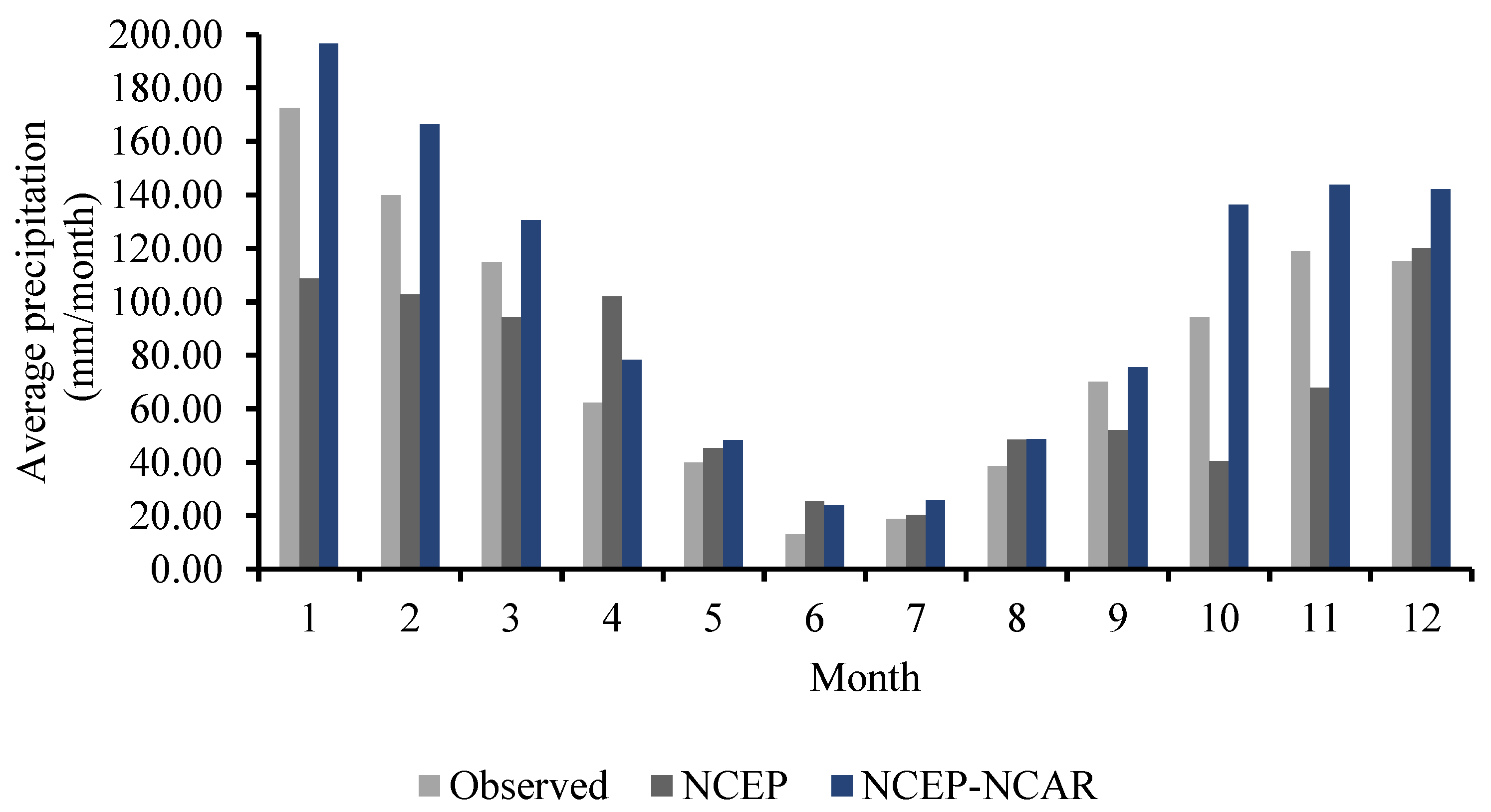
The calibration results indicate an acceptable correlation between the observed and the simulated monthly total rainfall and average Tmax and Tmin (Figure 2 and Figure 3). Different predictors for both air temperature calibration results follow a similar behaviour with modest biases between the simulated and observed data. The NCEP_NCAR predictors appear to slightly overestimate the maximum air temperature for almost the entire year. For Tmin, the results indicate a difference between the simulated Tmin and the local meteorological station data during winter than the rest of the year. The rainfall calibration results also show an overestimation using the NCEP_NCAR predictor for the whole year (Figure 2).

3.3. Validation of the SDSM Results

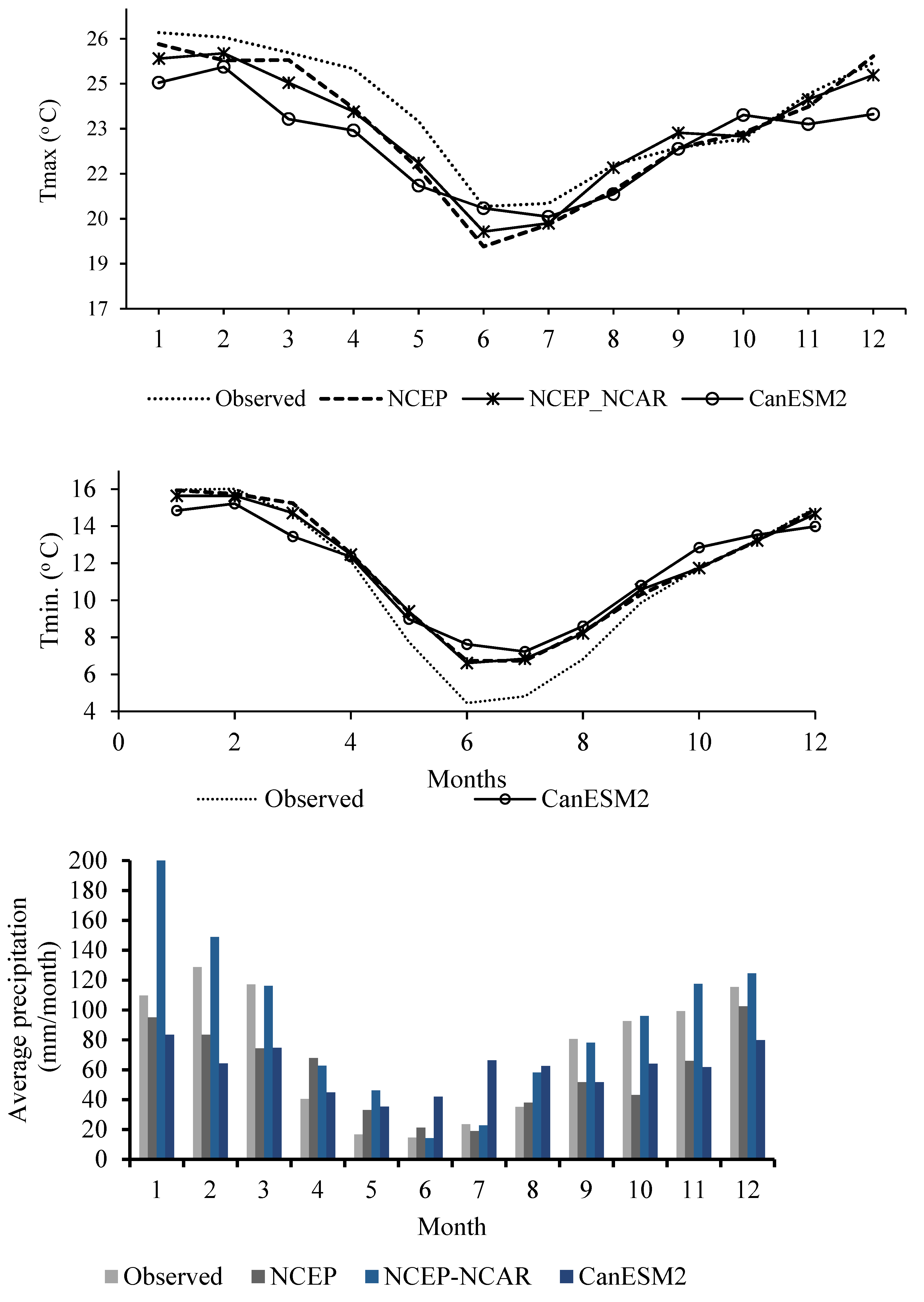
The measured 11-year period (1985–1996) data were used to validate the SDSM. In the validation process, three datasets were generated for the abovementioned period (1985-19960, extracting NCEP, NCEP-NCAR and CanESM2 variables). Figure 4 illustrates the measured monthly average Tmin, Tmax and rainfall. The statistical results of the simulated data are presented in Table 2. A similar pattern is observed in the simulated air temperature from different scenarios. However, the precipitation results indicate a huge difference between the simulated and measured data.
As presented in Table 2, the results suggest the better performance of the model in simulating air temperature relative to rainfall. The Tmin and Tmax deterministic metric results show satisfactory performance. For Tmin, the R2 and RMSE of NCEP are 0.99 and 0.98 °C, respectively, whereas for NCEP_NCAR the R2 and RMSE are 0.99 and 0.97 °C, respectively. For Tmax, the R2 and RMSE of NCEP are 0.87 and 0.93, respectively, while for NCEP_NCAR the R2 and RMSE are 0.82 and 0.92, respectively. The rainfall deterministic metric results indicate an acceptable performance with the R2 and RSME ranging between 0.56 and 0.76 and 28.53 and 40.05 mm, respectively. Similar behaviour is also observed for CanESM2 data in Table 2. The NSE results also indicate a good model fit for temperature simulations. However, NSE results show that the models simulate Tmin better than Tmax and precipitation. This may emanate from the fact that Tmin is highly influenced by greenhouse gas emissions through the greenhouse effect. Tmin dominates night time temperatures, and the greenhouse effect is apparent at night because night time temperatures are mainly regulated by infrared radiation emitted by the clouds and greenhouse gases back to the surface. The NSE results for air temperature range between 0.51 and 0.84 and 0.87 and 0.94 for Tmax and Tmin, respectively. For precipitation, NSE ranges between 0.30 and 0.53, suggesting the model’s poor performance for precipitation simulation. The results simulated by NCEP_NCAR and NCEP are superior to the CanESM2 models for all the predictands. These results suggest the better performance of SDSM in simulating air temperature compared to rainfall. Despite the biases detected between the simulated and measured data, a similar pattern is observed for all the predictands. The presented results suggest the capability of the abovementioned model to simulate air temperature and rainfall for the study site. Thus, this study employed CanESM2 for the simulation of Tmax, Tmin and rainfall

3.4. Validation Results after Bias Correction

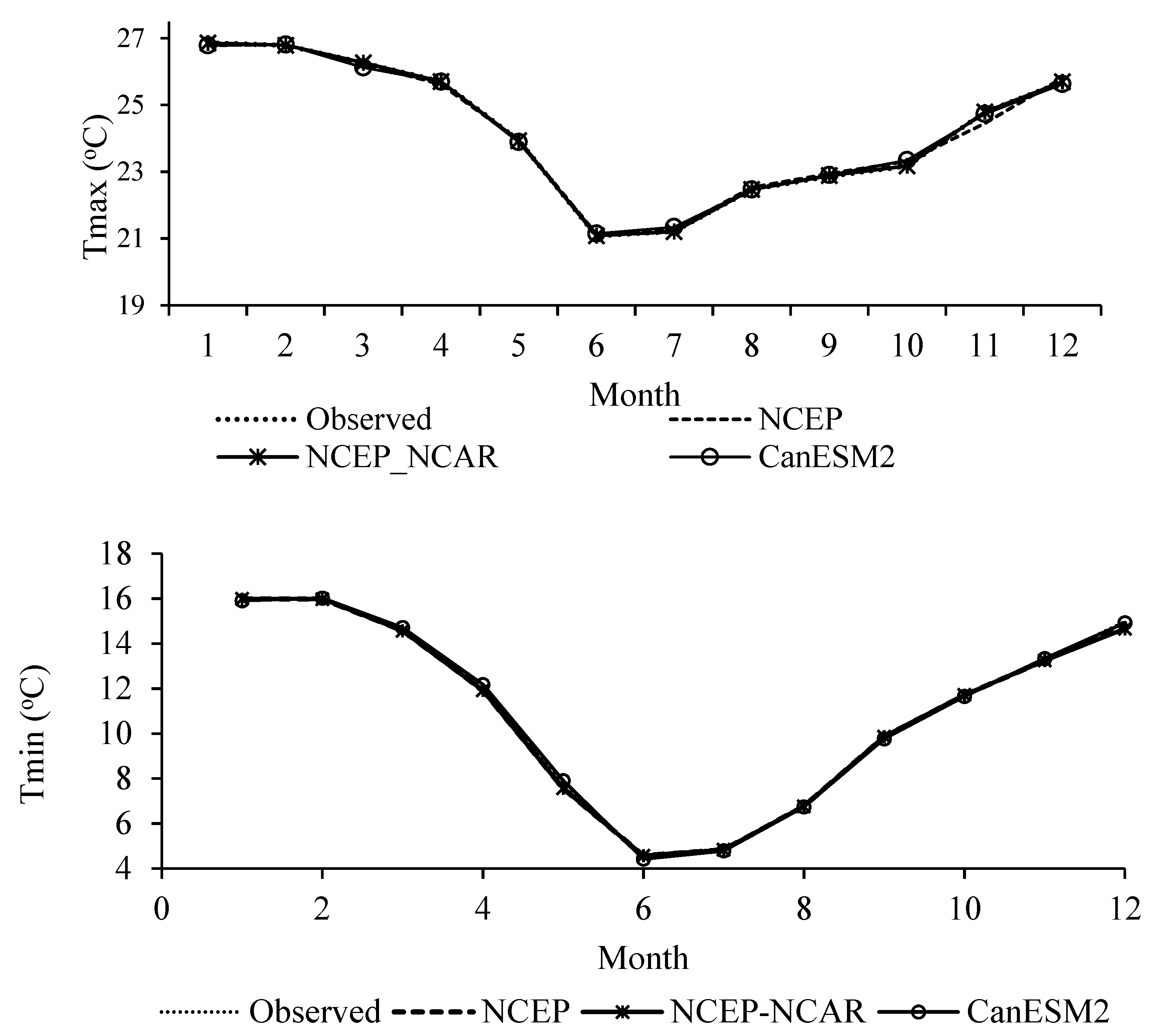
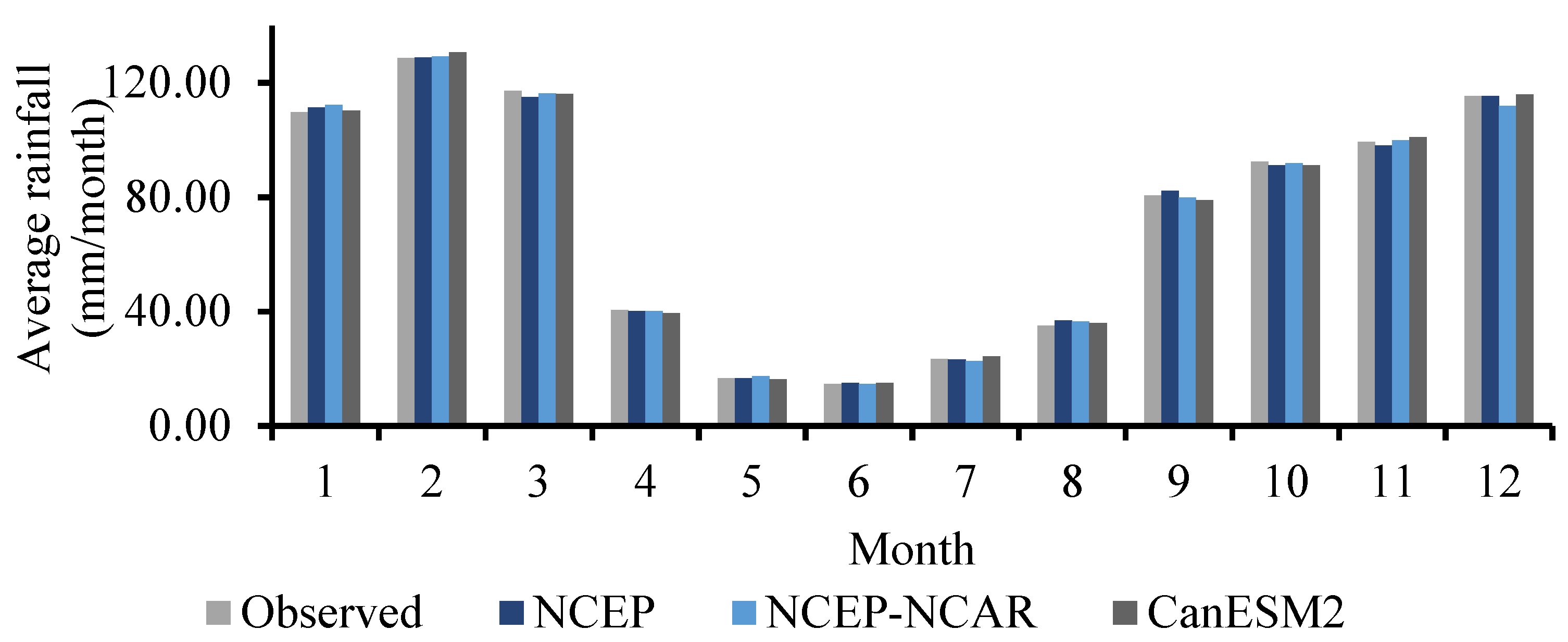
Although the model performance was deemed satisfactory for predicting future climate parameters, the results showed biases. The study applied bias correction techniques using Equations (1) and (2) to remove biases and improve validation results so as to obtain reliable future climate change projections. Table 3 displays the statistical results for Tmin, Tmax and rainfall after bias correction and the average monthly measured data, and bias-corrected simulated average monthly data are presented in Figure 5 and Figure 6. The results post-bias correction illustrate an improved R2 and reduced RMSE for both maximum and minimum air temperatures as well as rainfall.
The graphical presented results in Figure 5 and the statistical results in Table 3 show an improvement in SDSM in simulating Tmax, Tmin and rainfall after removing biases. The applied bias correction improved the results by reducing the difference between the generated and the measured data and hence ameliorated the correlation (Table 3). The CanESM2 results after bias correction were good enough to prove the applicability of SDSM for future climate projections in the study site. The RMSE and NSE values for monthly air temperature and rainfall show that CanEMS2 performance improved substantially. The RMSE values for the air temperature range between 0.08 and 0.22 °C while RMSE values for rainfall predictions range from 1.15 to 1.38 mm. The NSE values for all the variables were close to 1.00, suggesting the efficiency of the model in predicting the studied variables. The statistical analysis also affirmed that the SDSM performs better in simulating air temperature than rainfall. Based on the bias-corrected results and the graphical presented simulated and observed results, we attest that the CanESM2 model simulates climate variables fairly well in the study site. The plausible validation results and the satisfactory performance of the model demonstrate the capability of the model for projecting future Tmax, Tmin and rainfall in the study area.

3.5. Projected Trend of Average Maximum and Minimum Air Temperature and Annual Rainfall

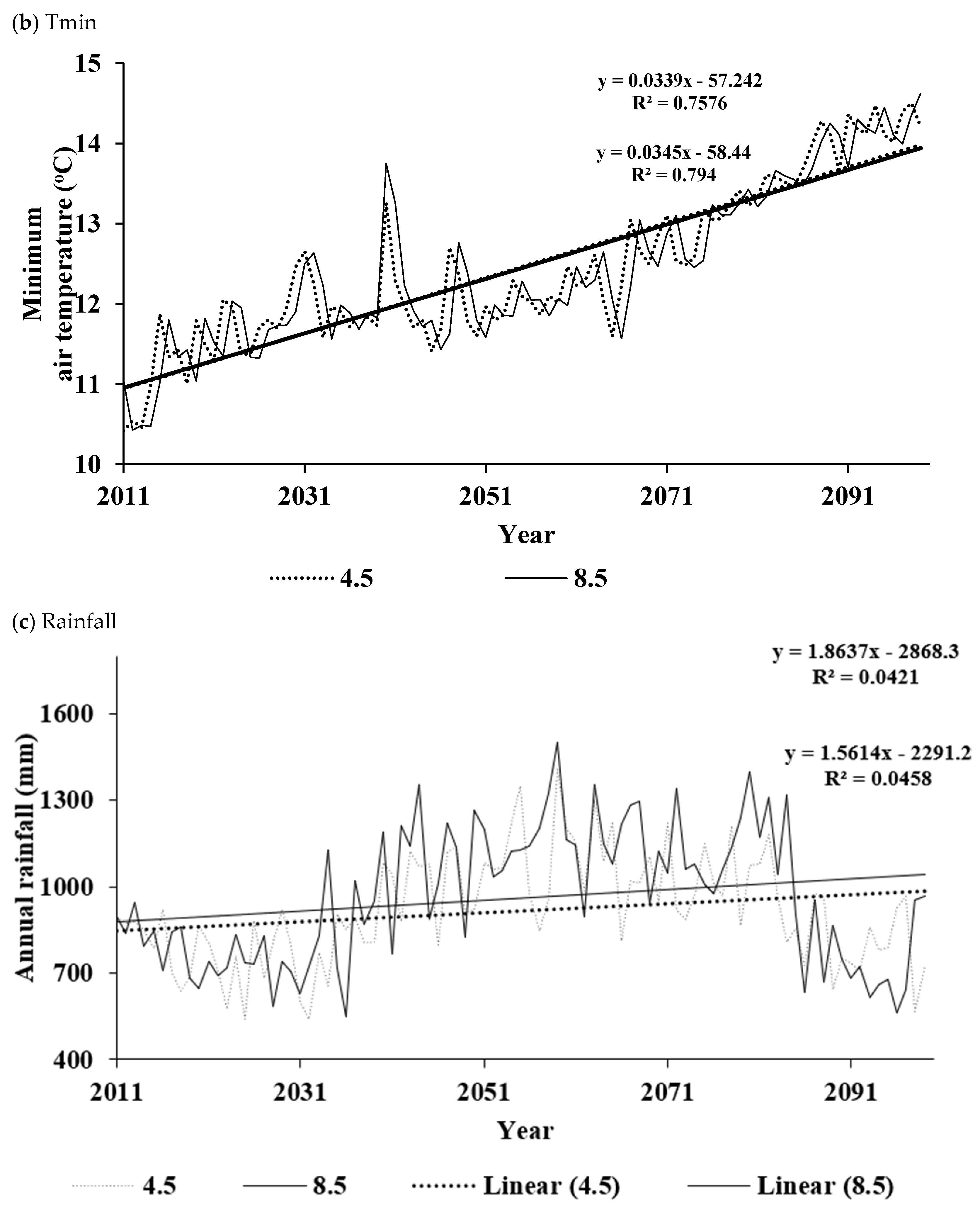
The projected trends of Tmax, Tmin and rainfall are presented in Figure 7. The results from different scenarios show a statistically significant positive trend for both maximum and minimum air temperature for the entire period studied. These findings correspond with the unanimity that climate change encompasses an increase in air temperature throughout the world. The CanESM2 RCP 8.5 and RCP 4.5 project an increase in Tmax from 24.0 to 28.5 °C and 23.8 to 26.5 °C, respectively, from 2011 to 2099. A maximum increase of about 4.5 °C relative to 2011 projected Tmax data is anticipated. For Tmin, an increase from 10.4 to 14.6 and 10.4 to 14.5 are projected by RCP 8.5 and RCP 4.5 °C, respectively. The results suggest that Tmax will increase drastically compared to Tmin and will reach the highest increase of about 4.5 °C in the 2080s. Rainfall predictions indicate a generally positive trend. The CanESM2 scenarios show a decreasing rainfall trend in the near future (2011–2040) and an increasing trend in the 2040s. After the 2040s, an increase in rainfall is observed and is expected to last until 2088. The rainfall projections indicate a decreasing trend for the study site after 2088. The RCP 8.5 and RCP 4.5 scenarios project the highest increase in total annual rainfall to about 1501 and 1162 mm, respectively.
The overall analysis of the results indicates a general increase in air temperature for all periods (the 2020s, 2040s, and 2080s) for the selected GCM scenarios (Table 4 and Table 5); however, the magnitude of these increases differed for the different scenarios. The scenario RCP 8.5 projected that the average monthly Tmax for the three periods would be 24.2, 24.6 and 26.8 °C, respectively. These values were found to be 1.2, 1.7 and 3.8 °C greater than the observed monthly average Tmax. The RCP 4.5 scenario also projected an increasing trend for all periods, indicating that average monthly Tmax would be 23.9, 24.2 and 25.1 °C, which are 0.98, 1.19 and 2.17 °C greater when compared with the observed monthly Tmax.
Temporal regression analysis was conducted to analyse the rate and the significance of changes in average yearly Tmax, Tmin and total rainfall. The results indicate an increasing rate of 0.009 to 0.164 and 0.022 to 0.052 °C annum−1 in Tmax based on RCP 4.5 and RPC 8.5 scenarios. The increase projected by RCP 8.5 was found to be statistically significant (p < 0.05) for all three prospective periods while the RCP 4.5 scenario projected a statistically significant increase in Tmax for the 2020s and 2040s only. A similar trend for the average monthly Tmin was projected for all the scenarios (Table 5). The results confirm the fact that the air temperature will continue to increase for the entire period studied. However, the Tmin results suggest similar patterns for RCP4.5 and RCP 8.5 scenarios. These results are thought-provoking considering that the RCP 8.5 scenario is likely to cause the highest increase in air temperature [1].
Although air temperature projections indicate a clear upward trend, rainfall projections display an undulating rainfall pattern for the study period. The model shows that the study area will receive the highest rainfall during the 2040s (Table 6). The results suggest an increasing rate of 1.989 to 4.373 mm annum−1 based on CanESM2 RCP 4.5 and RCP8 8.5, respectively, during the 2040s. However, the increase projected by CanESM2 was statistically insignificant, whereas the decreases were found to be statistically significant. The summary of the projected rainfall trend for the respective periods is presented in Table 6.

4. Discussion

4.1. Projected Air Temperature

All the CanESM2 scenarios project a continuous increase in air temperature for the study site reaching the highest in the 2080s. Based on the CanESM2 scenarios, the overall change for Tmin reveals that for P1 and P2 Tmin increases at a faster rate than Tmax, suggesting warmer nights. These results concur with various studies worldwide which confirmed night-time temperature increases, thus causing a significant reduction in cool nights [47,48]. However, for the study site, a statistically significant decreasing Tmin is projected for the 2040s, which indicates a relatively low magnitude of change compared to the observed period. These findings are consistent with other downscaling studies carried out across the globe and in southern Africa suggesting an increasing air temperature under global warming conditions [49,50,51] and South Africa [11,52]. The study results suggest that Tmin will likely follow the same pattern for both scenarios. Although unexpected, previous studies have also found similar results [21,53]. Global warming is a result of increased greenhouse gases (GHG) in the atmosphere. A high concentration of GHG in the atmosphere tends to absorb the heat emitted by the soil and sea surfaces and reradiate about 30% back to the surface, thus causing an increase in atmospheric and surface temperature. The greenhouse gases behave like a mantle absorbing infrared radiation and preventing it from escaping into outer space, thus causing the Earth’s atmosphere and surface to heat up. Global warming is mainly caused by the human-enhanced GHG effect. Human-induced GHGs result from several activities which include the burning of fossil fuels, use of aerosols and increased number and use of vehicles. These activities often increase the concentration of greenhouse gases such as carbon dioxide, methane and nitrous oxide as well as chlorofluorocarbons (CFCs) in the atmosphere [1].
There is a direct relationship between high air temperatures and the occurrence of extreme heat events which negatively affect crop growth and agricultural yields. For instance, sugarcane is sensitive to warmer minimum air temperatures as they tend to encourage flowering, which restricts the crop from growing [54]. Increasing air temperatures are harmful to both the environment and human life. The heat from high temperatures causes an increase in evapotranspiration, leading to the subsequent decrease in available soil moisture. High air temperatures are also associated with the preponderance of heat waves, wildfires and intense storms. The future scenario forcings project an increase in heatwave events to about 20–80 days annually relative to a maximum of 4–5 days under current conditions [49]. This implies that increasing air temperature due to climate change is not only challenging agricultural production but also biological life. Furthermore, high air temperatures coinciding with a limited supply of water to plants will result in great crop failures, hence low crop yields. A reduction in crop yield implies a substantial loss for the community considering that the entire community is either directly or indirectly involved in agriculture production by leasing out their land for income generation [55].

4.2. Projected Rainfall

The CanESM2 shows a general increase in rainfall, although a potential decrease in rainfall is projected for the 2020s and 2080s. The decrease in the rainfall trend over 1921 to 2015 has also been observed in the nearby weather station [12] and in South Africa, despite the lack of spatial coherence [11]. These results concur with previous studies which discovered an increase in the frequency and intensity of drought in southern Africa from 1960 to 2007 [56]. The projected annual projected change in rainfall indicates that the study site will experience a statistically significant decreasing trend in the 2080s. The study’s findings correspond with previous studies which projected an increase in drought occurrence in southern Africa [6] and Limpopo [57], as well as the prevalence of drought events in South Africa in the 2020s [12]. Trenberth [58] affirms that an increase in the atmospheric heat due to global warming will increase the ability of the air to hold water vapour, thus subsequently leading to an increase in potential evapotranspiration. An increase in potential evapotranspiration will in turn induce changes in the hydrological cycle, resulting in more precipitation extremes [57,59]. As the atmospheric moisture content consistently increases, extreme rainfall becomes more intense. The modelled extreme rainfall events are likely to be over a short duration. Previous studies confirm that sub-daily rainfall extremes are intensifying due to climate change [60]. The observed increase in short-duration extreme rainfall can be attributed to the convective cloud feedback. However, the modelled rainfall trend’s temporal heterogeneity may result from the fact that temperature may not necessarily be the only factor determining the available atmospheric humidity. The observations indicate that some rainfall intensities may be promoted by local-in-storm effects [61] and urbanization [62].
The substantial increase in the frequency of extreme rainfall events implies the lack of rainfall distribution throughout the rainfall season. This corresponds with the findings of Kruger [7], who indicated that under climate change, some parts of South Africa tend to experience longer dry periods, owing to an increase in sporadic heavy rainfall events. The implication is that the rainfall season may experience both dry and wet periods. The increased frequency of dry periods has adverse impacts on regional food availability and security [63,64]. The anticipated decrease in rainfall poses a threat to the sustainability of small-scale farming considering that they mainly rely on dryland agriculture. With the prevalence of dry condition events, most households in the study sites often experience major crop failures and yield as well as livestock losses, thus increasing poverty and food insecurity. Even though small-scale farmers in South Africa have been able to sustain livelihood under adverse conditions, their ability to deal with the projected climate extremes is uncertain. It has always been a serious challenge to recover from such losses, especially for crop farmers who often fail to measure climate-related crop losses which are required for obtaining drought relief funds from the government.

5. Conclusions

This study employed meteorological data from a specific weather station to examine future climate change. The canESM2 results indicate an upward air temperature trend throughout the study period. The projected increase in air temperature is concerning considering the high dependence of agricultural communities in the study site on rainfed agricultural production. A continuous increase in air temperature is likely to induce an increase in evapotranspiration, which could result in a downfall of small-scale sugarcane farming if farmers fail to adapt to such changes. The study results emphasize the need to devise climate change impact adaptation policies that address agricultural rural communities so as to manage and mitigate these adverse effects. Given the projected climate changes, small-scale sugarcane farmers must consider investing in heat-resistant varieties as a coping strategy.
It should be noted that by the nature of the study, the results are site-specific and have used projections of CanESM2 (RCP4.5 and RCP8.5). The study results present an opportunity for possible future research that would employ more meteorological stations across the province and utilize an ensemble from various climate models to enable a complete description of the potential impacts of climate change on air temperature and rainfall. It will prove the usefulness of GCMs in the assessment of uncertainties associated with the projections and provide improved results for decision makers. This research provides insight into the statistical downscaling technique and climate model data used to understand the potential risk associated with climate change at the local level.

Author Contributions

In completing the manuscript, Z.N.-M. and M.J.S. conceptualized the study. ZNM collected and analysed the data. Z.N.-M. and M.J.S. produced the first draft of the manuscript. All authors read the first drafts of the manuscript. All authors have read and agreed to the published version of the manuscript.

Funding

This research received no external funding.

Institutional Review Board Statement

Not applicable.

Informed Consent Statement

Not applicable.

Data Availability Statement

The datasets used or analysed during the current study are available from the provided websites.

Acknowledgments

The author acknowledges the South African Sugarcane Research Institute (SASRI) for providing data used in this study. In addition, I would like to extend my gratitude to R. L. Wilby from Loughborough University, UK, for providing the SDSM software and NCEP reanalysis datasets.

Conflicts of Interest

The authors declare no conflict of interest.

References

  1. IPCC. Climate Change 2013–The Physical Science Basis. Contribution of Working Group I to the Fifth Assessment Report of the Intergovernmental Panel on Climate Change; Cambridge University Press: Cambridge, UK; New York, NY, USA, 2014. [Google Scholar]
  2. Giorgi, F.; Raffaele, F.; Coppola, E. The response of precipitation characteristics to global warming from global and regional climate projections. Earth Syst. Dyn. 2019, 10, 73–89. [Google Scholar] [CrossRef]
  3. Stagl, J.; Mayr, E.; Koch, H.; Hattermann, F.F.; Huang, S. Effects of climate change on the hydrological cycle in Central and Eastern Europe. In Managing Protected Areas in Central and Eastern Europe under Climate Change; Rannow, S., Neubert, M., Eds.; Advances in Global Change Research; Springer: Dordrecht, The Netherlands, 2014; Volume 58, pp. 31–43. [Google Scholar]
  4. New, M.; Hewitson, B.; Stephenson, D.B.; Tsiga, A.; Kruger, A.; Manhique, A.; Gomez, B.; Coelho, C.A.S.; Masisi, D.N.; Kululanga, E. Evidence of trends in daily climate extremes over southern and West Africa. J. Geophys. Res. Atmos. 2006, 111, D14102. [Google Scholar] [CrossRef]
  5. Ujeneza, E.L.; Abiodun, B.J. Drought regimes in Southern Africa and how well GCMs simulate them. Clim. Dyn. 2015, 44, 1595–1609. [Google Scholar] [CrossRef]
  6. Abiodun, B.J.; Makhanya, N.; Petja, B.; Abatan, A.A.; Oguntunde, P.G. Future projection of droughts over major river basins in Southern Africa at specific global warming levels. Theor. Appl. Climatol. 2019, 139, 1785–1799. [Google Scholar] [CrossRef]
  7. Kruger, A.C. Observed trends in daily precipitation indices in South Africa: 1910–2004. Int. J. Climatol. 2006, 26, 2275–2285. [Google Scholar] [CrossRef]
  8. Kruger, A.C.; Shongwe, S. Temperature trends in South Africa: 1960–2003. Int. J. Climatol. 2004, 24, 1929–1945. [Google Scholar] [CrossRef]
  9. Edossa, D.C.; Woyessa, E.E.; Welderufael, W.A. Analysis of droughts in the central region of South Africa and their association with SST anomalies. Int. J. Atmos. Sci. 2014, 2014, 508953. [Google Scholar] [CrossRef]
  10. Gbetibouo, G.; Hassan, R. Measuring the economic impact of climate change on major South African field crops: A Ricardian approach. Glob. Planet. Change 2005, 47, 143–152. [Google Scholar] [CrossRef]
  11. Mackellar, N.; New, M.; Jack, C. Observed and modelled trends in rainfall and temperature for South Africa: 1960—2010. S. Afr. J. Sci. 2014, 110, 51–63. [Google Scholar] [CrossRef]
  12. Kruger, A.C.; Nxumalo, M. Historical rainfall trends in South Africa: 1921–2015. Water SA 2017, 43, 285–297. [Google Scholar] [CrossRef] [Green Version]
  13. Wilby, R.; Dawson, C.; Murphy, C.; O’Connor, P.; Hawkins, E. The Statistical DownScaling Model—Decision Centric (SDSM-DC): Conceptual basis and applications. Clim. Res. 2014, 61, 259–276. [Google Scholar] [CrossRef]
  14. Dorji, S.; Herath, S.; Mishra, B. Future climate of Colombo downscaled with SDSM-neural network. Climate 2017, 5, 24. [Google Scholar] [CrossRef]
  15. Li, D.; Zou, L.; Zhou, T. Extreme climate event changes in China in the 1.5 and 2 °C warmer climates: Results from statistical and dynamical downscaling. J. Geophys. Res. Atmos. 2018, 123, 215–230. [Google Scholar] [CrossRef]
  16. Boé, J.; Terray, L.; Habets, F.; Martin, E. Statistical and dynamical downscaling of the Seine basin climate for hydro-meteorological studies. Int. J. Climatol. 2007, 27, 1643–1655. [Google Scholar] [CrossRef]
  17. Lee, J.-H.; Kwon, H.-H.; Jang, H.-W.; Kim, T.-W. Future changes in drought characteristics under extreme climate change over South Korea. Adv. Meteorol. 2016, 2016, 9164265. [Google Scholar] [CrossRef]
  18. Jang, D. Assessment of meteorological drought indices in Korea using RCP 8.5 scenario. Water 2018, 10, 283. [Google Scholar] [CrossRef]
  19. Saymohammadi, S.; Zarafshani, K.; Tavakoli, M.; Mahdizadeh, H.; Amiri, F. Prediction of climate change induced temperature and precipitation: The case of Iran. Sustainability 2017, 9, 146. [Google Scholar] [CrossRef]
  20. Leng, G.; Tang, Q.; Rayburg, S. Climate change impacts on meteorological, agricultural and hydrological droughts in China. Glob. Planet. Change 2015, 126, 23–34. [Google Scholar] [CrossRef]
  21. Feyissa, G.; Zeleke, G.; Bewket, W.; Gebremariam, E. Downscaling of future temperature and precipitation extremes in Addis Ababa under climate change. Climate 2018, 6, 58. [Google Scholar] [CrossRef]
  22. Emami, F.; Koch, M. Evaluation of statistical-downscaling/bias-correction methods to predict hydrologic responses to climate change in the Zarrine River Basin, Iran. Climate 2018, 6, 30. [Google Scholar] [CrossRef] [Green Version]
  23. Mahmood, R.; Babel, M.S. Evaluation of SDSM developed by annual and monthly sub-models for downscaling temperature and precipitation in the Jhelum basin, Pakistan and India. Theor. Appl. Climatol. 2013, 113, 27–44. [Google Scholar] [CrossRef]
  24. Pinto, I.; Lennard, C.; Tadross, M.; Hewitson, B.; Dosio, A.; Nikulin, G.; Panitz, H.-J.; Shongwe, M.E. Evaluation and projections of extreme precipitation over southern Africa from two CORDEX models. Clim. Change 2016, 135, 655–668. [Google Scholar] [CrossRef]
  25. Dookie, N.; Chadee, X.T.; Clarke, R.M. Trends in extreme temperature and precipitation indices for the Caribbean small islands: Trinidad and Tobago. Theor. Appl. Climatol. 2018, 136, 31–44. [Google Scholar] [CrossRef]
  26. Dennis, I.; Dennis, R. Climate Change Vulnerability Index for South African Aquifers. Water SA 2012, 38, 417–426. [Google Scholar] [CrossRef]
  27. Stats, S.A. Statistical Release: Mid-Year Population Estimates; Statistics South Africa: Pretoria, South Africa, 2016. [Google Scholar]
  28. Hitayezu, P.; Zegeye, E.W.; Ortmann, G.F. Some aspects of agricultural vulnerability to climate change in the KwaZulu-Natal Midlands, South Africa: A systematic review. J. Hum. Ecol. 2014, 48, 347–356. [Google Scholar] [CrossRef]
  29. Hitayezu, P.; Wale, E.; Ortmann, G. Assessing farmers’ perceptions about climate change: A double-hurdle approach. Clim. Risk Manag. 2017, 17, 123–138. [Google Scholar] [CrossRef]
  30. Kollongei, K.J.; Lorentz, S.A. Connectivity influences on nutrient and sediment migration in the Wartburg catchment, KwaZulu-Natal Province, South Africa. Phys. Chem. Earth Parts A/B/C 2014, 67, 12–22. [Google Scholar] [CrossRef]
  31. Bureau for Food and Agricultural Policy (BFAP). Understanding the Factors That Have Impacted on Cane Production in the South African Sugar Industry. Retrieved April 26, 2019. 2014. Available online: https://www.bfap.co.za/wp-content/uploads/2018/08/2014_Understanding-the-Factors-That-Have-Impacted-on-Cane-Production.pdf (accessed on 19 July 2018).
  32. Mahlangu, I.; Lewis, F. Social and institutional constraints to the production of sugarcane by small-scale growers in the Amatikulu catchment. Proc. S. Afr. Sugar Technol. Assoc. 2008, 81, 128–132. [Google Scholar]
  33. Stöckle, C.O.; Campbell, G.S.; Nelson, R. ClimGen manual. In Biological Systems Engineering Department; Washington State University: Pullman, WA, USA, 1999. [Google Scholar]
  34. Gebremeskel, S.; Liu, Y.B.; De Smedt, F.; Hoffmann, L.; Pfister, L. Analysing the effect of climate changes on streamflow using statistically downscaled GCM scenarios. Int. J. River Basin Manag. 2004, 2, 271–280. [Google Scholar] [CrossRef]
  35. Government of Canada. HadCM3 Predictors: A2(a) and B2(a) Experiments. 2019. Available online: http://climate-scenarios.canada.ca/?page=pred-hadcm3#archived (accessed on 15 March 2018).
  36. Wilby, R.; Dawson, C.; Barrow, E. SDSM—A decision support tool for the assessment of regional climate change impacts. Environ. Model. Softw. 2002, 17, 145–157. [Google Scholar] [CrossRef]
  37. Wilby, R.L.; Dawson, C.W. The Statistical DownScaling Model: Insights from one decade of application. Int. J. Climatol. 2013, 33, 1707–1719. [Google Scholar] [CrossRef]
  38. Mahmood, R.; Babel, M.S.; Shaofeng, J.I.A. Assessment of temporal and spatial changes of future climate in the Jhelum river basin, Pakistan and India. Weather Clim. Extrem. 2015, 10, 40–55. [Google Scholar] [CrossRef]
  39. Chu, J.T.; Xia, J.; Xu, C.-Y.; Singh, V.P. Statistical downscaling of daily mean temperature, pan evaporation and precipitation for climate change scenarios in Haihe River, China. Theor. Appl. Climatol. 2010, 99, 149–161. [Google Scholar] [CrossRef]
  40. Nury, A.H.; Alam, M.J.B. Performance study of global circulation model HadCM3 using SDSM for temperature and rainfall in North-Eastern Bangladesh. J. Sci. Res. 2013, 6, 87–96. [Google Scholar] [CrossRef]
  41. Mirgol, B.; Nazari, M. Possible scenarios of winter wheat yield reduction of dryland Qazvin Province, Iran, based on prediction of temperature and precipitation till the end of the century. Climate 2018, 6, 78. [Google Scholar] [CrossRef]
  42. Tahir, T.; Hashim, A.M.; Yusof, K.W. Statistical downscaling of rainfall under transitional climate in Limbang River Basin by using SDSM. In IOP Conference Series: Earth Environmental Sciences; IOP Publishing: Bristol, UK, 2018; Volume 140, p. 012037. [Google Scholar] [CrossRef]
  43. Liu, J.; Chen, S.; Li, L.; Li, J. Statistical downscaling and projection of future air temperature changes in Yunnan Province, China. Adv. Meteorol. 2017, 2017, 2175904. [Google Scholar] [CrossRef]
  44. Salzmann, N.; Frei, C.; Vidale, P.-L.; Hoelzle, M. The application of Regional Climate Model output for the simulation of high-mountain permafrost scenarios. Glob. Planet. Change 2007, 56, 188–202. [Google Scholar] [CrossRef]
  45. Schär, C.; Vidale, P.L.; Lüthi, D.; Frei, C.; Häberli, C.; Liniger, M.A.; Appenzeller, C. The role of increasing temperature variability in European summer heatwaves. Nature 2004, 427, 332–336. [Google Scholar] [CrossRef]
  46. Hashmi, M.Z.; Shamseldin, A.Y.; Melville, B.W. Comparison of SDSM and LARS-WG for simulation and downscaling of extreme precipitation events in a watershed. Stoch. Environ. Res. Risk Assess. 2011, 25, 475–484. [Google Scholar] [CrossRef]
  47. Alexander, L.V.; Zhang, X.; Peterson, T.C.; Caesar, J.; Gleason, B.; Klein Tank, A.M.G.; Haylock, M.; Collins, D.; Trewin, B.; Rahimzadeh, F.; et al. Global observed changes in daily climate extremes of temperature and precipitation. J. Geophys. Res. Atmos. 2006, 111, D05109. [Google Scholar] [CrossRef] [Green Version]
  48. Donat, M.G.; Alexander, L.V.; Yang, H.; Durre, I.; Vose, R.; Dunn, R.J.H.; Willett, K.M.; Aguilar, E.; Brunet, M.; Caesar, J.; et al. Updated analyses of temperature and precipitation extreme indices since the beginning of the twentieth century: The HadEX2 dataset. J. Geophys. Res. Atmos. 2013, 118, 2098–2118. [Google Scholar] [CrossRef]
  49. James, R.; Washington, R. Changes in African temperature and precipitation associated with degrees of global warming. Clim. Change 2013, 117, 859–872. [Google Scholar] [CrossRef]
  50. Engelbrecht, F.; Adegoke, J.; Bopape, M.-J.; Naidoo, M.; Garland, R.; Thatcher, M.; McGregor, J.; Katzfey, J.; Werner, M.; Ichoku, C. Projections of rapidly rising surface temperatures over Africa under low mitigation. Environ. Res. Lett. 2015, 10, 085004. [Google Scholar] [CrossRef]
  51. Dosio, A. Projection of temperature and heat waves for Africa with an ensemble of CORDEX Regional Climate Models. Clim. Dyn. 2017, 49, 493–519. [Google Scholar] [CrossRef]
  52. Kruger, A.C.; Nxumalo, M. Surface temperature trends from homogenized time series in South Africa: 1931–2015. Int. J. Climatol. 2017, 37, 2364–2377. [Google Scholar] [CrossRef]
  53. Kidanemariam, S.; Goitom, H.; Desta, Y. Coupled application of R and WetSpa models for assessment of climate change impact on streamflow of Werie Catchment, Tigray, Ethiopia. J. Water Clim. Change 2021, 12, 916–936. [Google Scholar] [CrossRef]
  54. Climate Change 2014–Impacts, Adaptation, and Vulnerability: Regional Aspects; Field, C.B. (Ed.) Cambridge University Press: Cambridge, UK, 2014. [Google Scholar]
  55. Swayimana Small-Scale Farmers. Personal Communication, 2019.
  56. Nhamo, L.; Mabhaudhi, T.; Modi, A.T. Preparedness or Repeated Short-Term Relief Aid? Building Drought Resilience through Early Warning in Southern AFRICA. Water SA 2019, 45, 75–85. [Google Scholar]
  57. Botai, C.M.; Botai, J.O.; Zwane, N.N.; Hayombe, P.; Wamiti, E.K.; Makgoale, T.; Murambadoro, M.D.; Adeola, A.M.; Ncongwane, K.P.; de Wit, J.P.; et al. Hydroclimatic Extremes in the Limpopo River Basin, South Africa, under Changing Climate. Water 2020, 12, 3299. [Google Scholar] [CrossRef]
  58. Trenberth, K.E. The impact of climate change and variability on heavy precipitation, floods, and droughts. In Encyclopedia of Hydrological Sciences; Anderson, M.G., Ed.; Wiley: Hoboken, NJ, USA, 2006; pp. 1–11. [Google Scholar] [CrossRef]
  59. Abiodun, B.J.; Adegoke, J.; Abatan, A.A.; Ibe, C.A.; Egbebiyi, T.S.; Engelbrecht, F.; Pinto, I. Potential impacts of climate change on extreme precipitation over four African coastal cities. Clim. Change 2017, 143, 399–413. [Google Scholar] [CrossRef]
  60. Fowler, H.J.; Wasko, C.; Prein, A.F. Intensification of short-duration rainfall extremes and implications for flood risk: Current state of the art and future directions. Philos. Trans. R. Soc. A 2021, 379, 20190541. [Google Scholar] [CrossRef]
  61. Lenderink, G.; Barbero, R.; Loriaux, J.M.; Fowler, H.J. Super-Clausius-Clapeyron scaling of extreme hourly convective precipitation and its relation to large-scale atmospheric conditions. J. Clim. 2017, 30, 6037–6052. [Google Scholar] [CrossRef]
  62. Li, Y.; Fowler, H.J.; Argüeso, D.; Blenkinsop, S.; Evans, J.P.; Lenderink, G.; Yan, X.; Guerreiro, S.B.; Lewis, E.; Li, X.F. Strong intensification of hourly rainfall extremes by urbanization. Geophys. Res. Lett. 2020, 47, e2020GL088758. [Google Scholar] [CrossRef]
  63. Calow, R.C.; MacDonald, A.M.; Nicol, A.L.; Robins, N.S. Ground water security and drought in Africa: Linking availability, access, and demand. Groundwater 2010, 48, 246–256. [Google Scholar] [CrossRef] [PubMed]
  64. Ngcamu, B.S.; Chari, F. Drought influences on food insecurity in Africa: A Systematic literature review. Int. J. Environ. Res. Public Health 2020, 17, 5897. [Google Scholar] [CrossRef] [PubMed]
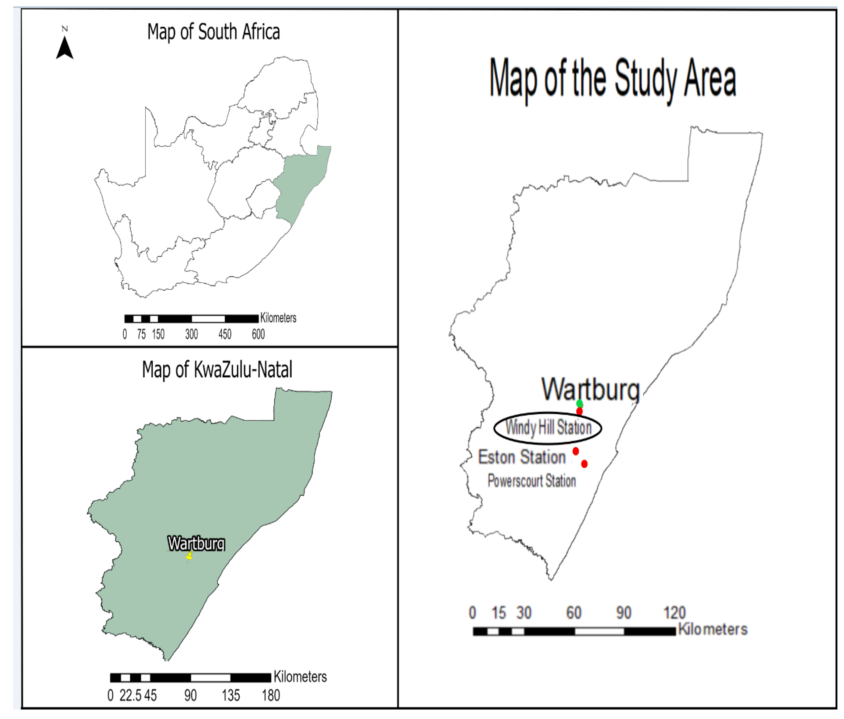
Figure 1. Location Map of the Wartburg area for the study.
Sustainability 14 10682 g001
Figure 2. Comparison of monthly observed and simulated Tmax and Tmin using SDSM for the calibration period 1966 to 1984.
Sustainability 14 10682 g002
Figure 3. Comparison of monthly observed and simulated rainfall using SDSM for the period 1966 to 1984.
Sustainability 14 10682 g003
Figure 4. Validated Tmax, Tmin and rainfall before bias correction using SDSM for the validation period of 1985 to 1996.
Sustainability 14 10682 g004
Figure 5. Validation of monthly observed and simulated Tmax and Tmin after bias correction using SDSM for the validation period 1985 to 1996.
Sustainability 14 10682 g005
Figure 6. Validation of monthly observed and simulated rainfall after bias correction using SDSM for 1985 to 1996.
Sustainability 14 10682 g006
Figure 7. Projected future annual Tmax (a), Tmin (b) and rainfall (c) using SDSM from CanESM2 RCP 4.5 and RCP 8.5 scenarios for 2011–2099.
Sustainability 14 10682 g007aSustainability 14 10682 g007b
Table 1. Predictors that were considered for the projection of precipitation, Tmax and Tmin.
TminTmaxPrecipitation
NCEP_NCAR PredictorsPartial rp ValueNCEP_NCAR PredictorsPartial rp ValueNCEP_NCAR PredictorsPartial rp Value
Mean temperature at 2 m height (temp)0.4760.00Mean temperature at 2 m height (temp)0.6370.00Surface-specific humidity (shum)0.1990.00
Surface-specific humidity (shum)0.4370.00850 hPa zonal velocity (p_8u)0.3770.00500 hPa wind direction (p5th)0.1100.00
Surface airflow strength (p_f)0.0590.00Surface divergence (p_zh)0.3380.00850 hPa airflow strength (p_8f)0.1070.00
Surface vorticity (p_z)0.0230.05Mean sea level pressure (mslp)0.0270.020Surface meridional velocity (p_v)0.0940.00
NCEP PredictorsNCEP PredictorsNCEP Predictors
Mean temperature at 2 m height (temp)0.6110.00850 hPa zonal velocity (p_8u)0.5110.00Surface meridional velocity (p_v)0.1510.00
Surface-specific humidity (shum)0.4580.00Surface-specific humidity (shum)0.3880.00Surface-specific humidity (shum)0.1430.00
Surface airflow strength (p_f)0.2530.00Mean temperature at 2 m height (temp)0.3080.00500 hPa relative humidity (r500)0.1160.00
Surface vorticity (p_z)0.1730.00Mean sea level pressure (mslp)0.2490.00850 hPa airflow strength (p_8f)0.0430.03
Table 2. Before bias correction, statistical results for the comparison of the observed and simulated rainfall and the maximum and the minimum air temperatures for the validation period 1985–1996.
TmaxTminRainfall
MeanStd devRMSER2NSEMeanStd devRMSER2NSEMeanStd devRMSER2NSE
(°C)(°C)(°C) (°C)(°C)(°C) (mm)(mm)(mm)
Observed23.592.06 11.094.11 72.7643.56
CanEMS222.551.631.350.790.5111.622.821.430.970.8781.6049.9532.760.570.30
NCEP22.992.280.870.930.8211.733.420.980.990.9457.8427.9228.530.690.39
NCEP_NCAR23.021.990.820.920.8411.653.310.970.990.9491.0455.7740.050.760.53
Table 3. Statistical maximum and minimum air temperature and rainfall monthly results for the observed and simulated after bias correction for the validation period 1985–1996.
Tmax Tmin Rainfall
Mean
(°C)
Std Dev
(°C)
RMSE
(°C)
R2NSEMean
(°C)
Std Dev
(°C)
RMSE
(°C)
R2NSEMean
(mm)
Std Dev
(mm)
RMSE
(mm)
R2NSE
Observed23.592.06 11.044.22 72.7643.56
CanEMS223.772.090.200.990.9911.034.230.080.991.0072.8343.691.150.990.99
NCEP23.762.110.190.990.9910.994.200.100.990.9972.7943.281.160.990.99
NCEP_NCAR23.782.100.220.990.9810.974.180.131.000.9972.6843.341.380.990.99
Table 4. Overall change of Tmax for future climate generated using CanESM2 model scenarios (changes based on the 1966–1996 Tmin mean).
GCM ScenariosPeriodsOverall Tmax ChangeSlope (annum−1)Significance < 0.05
Observed1966–199622.96
RCP 4.52020s (P1)23.94
2040s (P2)24.15
2080s (P3)25.13
°C change P1 vs. obs0.980.066p < 0.05
°C change P2 vs. obs1.190.167p < 0.05
°C change P3 vs. obs2.170.012p > 0.05
RCP 8.52020s (P1)24.17
2040s (P2)24.63
2080s (P3)26.80
°C change P1 vs. obs1.210.022p > 0.05
°C change P2 vs. obs1.670.074p < 0.05
°C change P3 vs. obs3.840.057p < 0.05
Table 5. Overall change of Tmin for future climate generated using CanESM2 model scenarios (changes based on the 1966–1996 Tmin mean).
GCM ScenariosPeriodsOverall Tmin ChangeSlope (annum−1)Significance < 0.05
Observed1966–199611.53
RCP 4.52020s (P1)13.13
2040s (P2)13.59
2080s (P3)13.87
°C change P1 vs. obs1.600.049p < 0.05
°C change P2 vs. obs2.060.025p < 0.05
°C change P3 vs. obs2.340.065p < 0.05
RCP 8.52020s (P1)13.33
2040s (P2)13.95
2080s (P3)15.19
°C change P1 vs. obs1.800.055p < 0.05
°C change P2 vs. obs2.420.012p < 0.05
°C change P3 vs. obs3.660.070p < 0.05
Table 6. Overall change of rainfall for future climate generated from CanESM2 model scenarios (changes based on the 1966–1996 rainfall mean).
GCM ScenariosPeriodsOverall Rainfall ChangeSlope (annum−1)Significance < 0.05
Observed1966–1996960.37
RCP 4.52020s (P1)782.61
2040s (P2)1063.49
2080s (P3)907.44
% change P1 vs. obs−18.510.687p > 0.05
% change P2 vs. obs10.741.979p > 0.05
% change P3 vs. obs−5.66−12.730p < 0.05
RCP 8.52020s (P1)799.27
2040s (P2)1138.85
2080s (P3)951.48
% change P1 vs. obs−16.772.842p > 0.05
% change P2 vs. obs18.584.373p > 0.05
% change P3 vs. obs−1.44−19.678p < 0.05
Publisher’s Note: MDPI stays neutral with regard to jurisdictional claims in published maps and institutional affiliations.