Research on Accurate Estimation Method of Eucalyptus Biomass Based on Airborne LiDAR Data and Aerial Images

Abstract

Forest biomass is a key index to comprehend the changes of ecosystem productivity and forest growth and development. Accurate acquisition of single tree scale biomass information is of great significance to the protection, management and monitoring of forest resources. LiDAR technology can penetrate the forest canopy and obtain information on the vertical structure of the forest. Aerial photography technology has the advantages of low cost and high speed, and can obtain information on the horizontal structure of the forest. Therefore, in this study, multispectral imagery and LiDAR data were integrated, and a part of the Zengcheng Forest Farm in Guangdong Province was selected as the study area. Large-scale and high-precision Eucalyptus biomass estimation research was gradually carried out by screening influencing factors and establishing models. This study compared and analysed the performance of multiple stepwise regression methods, random forest algorithms, support vector machine algorithms and decision tree algorithms for Eucalyptus biomass estimation to determine the best method for Eucalyptus biomass estimation. The results demonstrated that the accuracy of the model established by the machine learning method was higher than that of the linear regression model, and in the machine learning model, the random forest model had the best performance on both the training set (R² = 0.9346, RMSE = 8.8399) and the test set (R² = 0.8670, RMSE = 15.0377). RF was more suitable for the biomass estimation of Eucalyptus in this study. The spatial resolution of Eucalyptus biomass distribution was 0.05 m in this study, which had higher accuracy and was more accurate. It can provide data reference for the details about biomass distribution of Eucalyptus in the majority of provinces, and has certain practical reference significance.

1. Introduction

Forests are the most active habitat and reproduction area on earth, regulating the climate environment, known as the “lungs of the earth”, and play a pivotal role in the global carbon cycle, climate change and biodiversity [1,2,3]. In recent years, as global ecological problems such as volcanic eruptions, rising sea levels and locust plagues have become increasingly serious, countries have placed the conservation and monitoring of forest resources in a key strategic position [4,5]. Among the forest parameters, biomass indicators are particularly important, as they reveal the nature and state of forest ecosystems and are key indicators for understanding forest productivity [6]. In precision forestry, the accurate acquisition of single-tree-scale biomass information is of great significance for the refined management of forest information and the monitoring of forest growth and development.

Eucalyptus, with its wide range of growth and high yield per unit area, is planted in large numbers in the south of the country. Eucalyptus is a major forest tree species in China, with great economic value and an important component of our carbon sinks and stocks. With the large-scale planting of Eucalyptus, the area proportion of Eucalyptus in Guangdong and Guangxi ranks among the top in China. Moreover, accurate estimation of Eucalyptus biomass is essential to describe the biomass status of plantation forests in the southern region [7].

Currently, the common methods used for single wood scale biomass modelling are statistical based parametric modelling and non-parametric modelling. The parametric model method is primarily a regression analysis, where a linear relationship with the target is established by screening the factors. Thomas et al. investigated the correlation between quantile models for different sampling densities of point clouds and the above-ground biomass of single wood, demonstrating that the accuracy of biomass estimation with quantile models of point cloud density reached 0.91 [8]. Zheng developed a single wood-scale biomass model in the form of a power function based on data from a natural forest sample plot of Simao Pine, using single wood structural parameters (tree height, diameter at breast height, crown width, etc.) as factors [9]. Ou et al. used stepwise regression to estimate the biomass of Yunnan red bean fir, screening the factors of crown height and tree height, and the estimation accuracy was 92.36% [10]. The main non-parametric modelling approach commonly used is machine learning. Machine learning uses the advantages of computers in data mining to perform biomass estimation using a ‘black box’-like operation. Common methods include: random forest (Random Forest, RF), k-nearest neighbour (K-Nearest Neighbour, KNN), support vector machine (Supported Vector Regress, SVM), decision tree (Decision Tree, DT), maximum entropy (Maximum Entropy, Max Ent), artificial neural network (Artificial Neural Network, ANN), etc. Gleason et al. extracted the structural parameters of trees based on the acquired airborne LiDAR point clouds and used these parameters as independent variables for biomass modelling, comparing the accuracy of linear regression, RF, Cubist decision tree and SVR methods for single wood above-ground biomass estimation. The results demonstrated that the SVR estimation results had the highest accuracy [11]. Li combined DOM data with laser point cloud data to extract point cloud single wood information and factors such as vegetation index and texture from multispectral images, and compared the accuracy of Cubist, KNN, RF and SVR methods for biomass estimation, showing that the Cubist model had the best accuracy [12]. Zhang et al. estimated the biomass of a single tree in the Penobscot test forest in the United States based on random forest and support vector machine methods, which made the single tree biomass model more generalised and the estimation accuracy was higher [13].

In conclusion, most studies now reveal the estimation and distribution pattern of Eucalyptus biomass at the regional and stand scales to some extent, but there are few studies on biomass estimation at the individual tree scale. Moreover, there are many forest information data sources, each with its own advantages, and there are also many biomass estimation methods. How to effectively use a variety of data to accurately construct a single-tree-scale biomass estimation model and achieve large-scale and high-precision biomass estimation is a problem that needs to be solved at present. Therefore, this study combined the vertical structure information of trees (tree height, crown width, etc.) obtained from airborne LiDAR point cloud data with high-resolution multispectral imagery to achieve and complement the horizontal and vertical structure data of trees and improve the accuracy of single wood extraction and biomass estimation of eucalypts. This study took Eucalyptus, a strategic tree species in the southern region of China, as the research object, and combined the multi-spectral data obtained from LiDAR and high-resolution helicopters from Zengcheng Forestry Field in Guangzhou City to gradually carry out research on the accurate estimation of Eucalyptus biomass through single wood segmentation and the extraction of relevant biomass factors. This study contributes to the accurate estimation of Eucalyptus biomass in a large scale, plays an important role in describing the biomass status of plantation forests in southern China, and also provides technical and data references for other regional biomass estimation studies at the single-tree scale.

2. Study Area and Data Sources

2.1. Study Area

The study area is located in Zengcheng Forestry Field, Guangzhou City, Guangdong Province (23.292° to 23.369° N, 113.681° to 113.815° E), which is a state-owned forest, with a total area of about 2777.55 hm². The spring is cold and wet with more rainfall, and the summer is hot and muggy.

The region receives ample rainfall and there is little variation in temperature throughout the year, with an average annual temperature of around 22.7 °C, an average annual relative humidity of 79% and an annual precipitation of around 1890 mm. The forest cover is 89.3%, with lush vegetation growth. The vegetation is diverse, with the majority of forest species being soil and water conservation forests and fast-growing, productive timber forests, with a small amount of landscape forests and short rotation industrial timber forests. Tree species in the woodland are mostly trees, mainly found in Eucalyptus, Pinus massoniana, A. melanoxylon, Cunninghamia lanceolata, Pinus elliottii, Castanopsis fissa, etc. In view of the large area and wide distribution of Eucalyptus plantations in the whole forest, only a part of the area was selected for the study of Eucalyptus biomass, which covered an area of 11.11 hm². The geographical location and orthophoto of the study area are shown in Figure 1.

2.2. Data Sources

2.2.1. Image Data

The data used in this study was acquired via Bell Helicopter on 18 and 19 November 2019 and consisted mainly of aerial multispectral imagery and airborne LiDAR point cloud data (Figure 2.). Three routes were designed throughout the forest, with a helicopter flight altitude of 500 m, a 45% overlap in the side direction and a 65% overlap in the heading. The helicopter was equipped with a Feith camera with 100 million pixels with 3 bands of red, green and blue, taking more than 2900 images with a total data volume of more than 850 G and obtaining orthophotos with a ground resolution of up to 0.07 m. The laser sensor on board the helicopter was the Galaxy Prime Sensor, which was suitable for large mountainous areas and narrow terrain and had good spatial resolution, as shown in

Table 1. Sensor parameters.

Parameters	Specification
Flight height/m	500
Ground speed/kn	60
Mapping bandwidth/m	175
Laser wavelength/nm	1064
Pulse repetition rate/kHz	50~1000
Scanning view/(°)	10~60
Average point cloud density/(pts/m2)	180
Positioning and orientation systems	POS AV™ AP60 (OEM); 220-channel dual-frequency GNSS receiver; GNSS airborne antenna with iridium filter; Highly accurate AIMU (Type 57);

. The sun was shining at the time of data collection, with good light conditions, no cloud cover, clear and no wind, suitable for data collection operations. This study combined airborne LiDAR data with multispectral data to give full play to the advantages of high-resolution data, and the distribution of vegetation in the forest could be clearly and accurately obtained, providing a basis for high-precision Eucalyptus biomass estimation.

2.2.2. Sample Data

Eucalyptus field sample sites were sampled and obtained in November 2019, with an average sampling interval of more than 10 m. A total of 100 Eucalyptus trees were collected within the study area. The locations of the trees were located using GPS, and information on the diameter at breast height (DBH) and height of the Eucalyptus trees was measured and recorded in the field (

Table 2. Eucalyptus sample wood information.

Tree Number	Longitude	Latitude	DBH/cm	Height/m
1	113°47′22″ E	23°19′53″ N	35.00	23.80
2	113°47′28″ E	23°19′42″ N	20.30	17.00
3	113°47′29″ E	23°19′43″ N	7.50	7.80
4	113°47′29″ E	23°19′53″ N	18.40	14.80
5	113°47′25″ E	23°19′51″ N	4.00	3.10
…	…	…	…	…
98	113°47′24″ E	23°19′51″ N	19.00	16.20
99	113°47′28″ E	23°19′50″ N	13.60	14.20
100	113°47′22″ E	23°19′49″ N	23.50	19.00

). The average height of the 100 sampled Eucalypts was counted to be 13.19 m and the average diameter at breast height was 12.63 cm. In order to improve the accuracy of Eucalyptus biomass estimation, more sample points need to be obtained. In this study, 100 Eucalyptus sample points were manually interpreted visually using high-resolution orthophotos, and canopy and tree height information was recorded for the Eucalyptus sample points using a length measurement tool and canopy height. This part of the sample was only selected as a sample point for eucalypts if 100% information on location, crown size and height was determined to be available. The final 200 Eucalyptus trees sample data was shown in Figure 2.

In this research, we consulted the correlation between DBH and crown width of main timber forests in Guangdong Province given by Guangdong Provincial Investigation Institute, and obtained the relationship between measured DBH and crown width of Eucalyptus urophylla.

The correlation between diameter at breast height and crown width of the main timber forests in Guangdong Province was obtained by checking the correlation between the measured diameter at breast height and crown width of the Eucalyptus tailleaf (Equation (1)), based on which the diameter at breast height of these 100 Eucalyptus sample points was calculated to form a complete Eucalyptus sample.

$$\mathrm{C}=0.51539+0.17531\mathrm{D}$$

(1)

where C is the crown width in m, and D is the diameter at breast height in cm.

Biomass estimation was conducted based on the high precision Eucalyptus single wood obtained in the previous step. Based on the Eucalyptus sample data, the measured Eucalyptus biomass AGB was calculated according to the equation for calculating above-ground biomass of Eucalyptus spp. in Guangdong Province with a precision of R² = 0.953 (Equation (2)), as recorded in the manual on biomass modelling of major forest trees in China.

$${\mathrm{W}}_{\mathrm{a}}=0{.1882\mathrm{D}}^{2.1916}$$

(2)

where ${\mathrm{W}}_{\mathrm{a}}$ is the above-ground biomass of Eucalyptus in kg, and D is the diameter at breast height in cm.

3. Research Methods

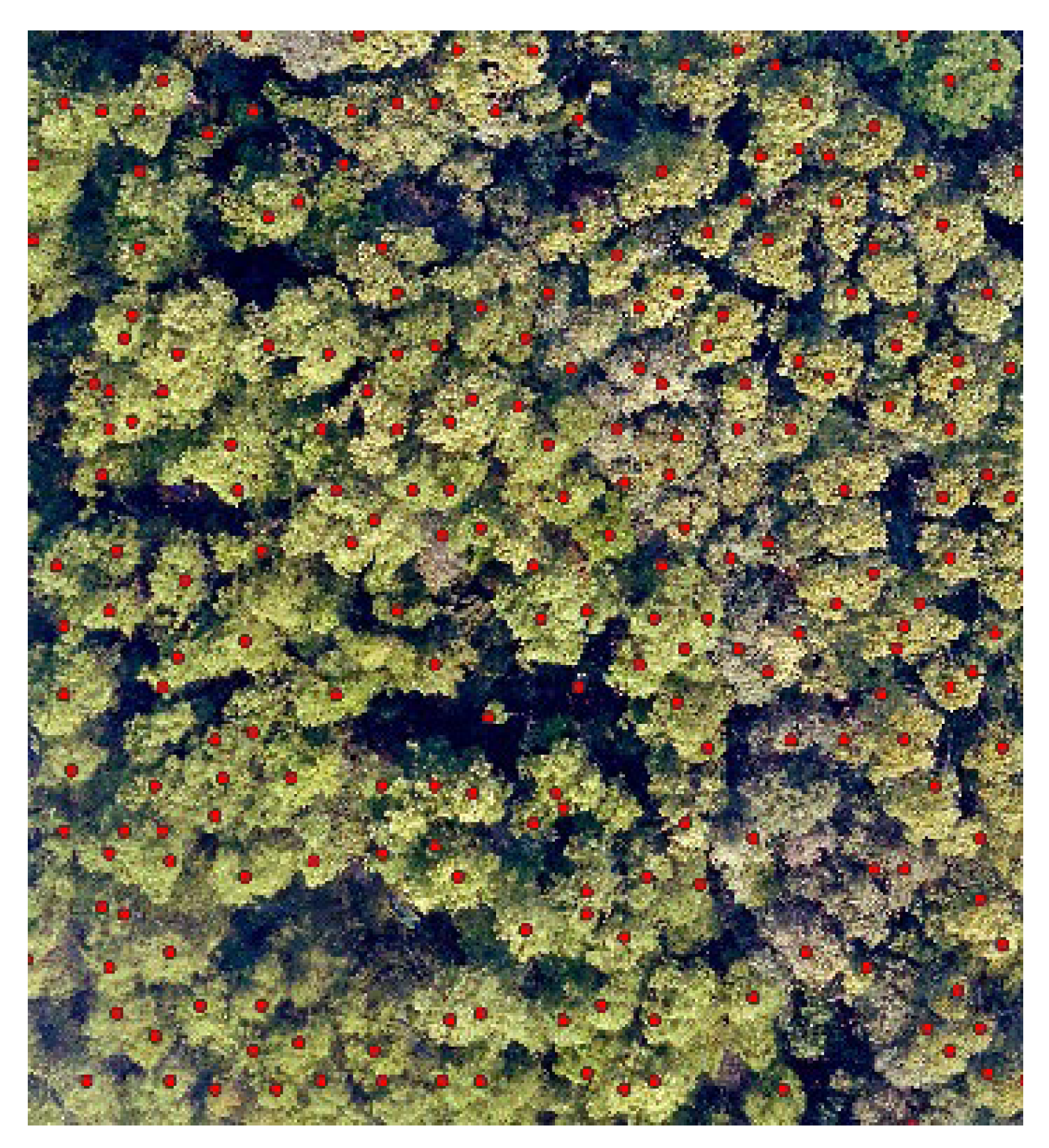
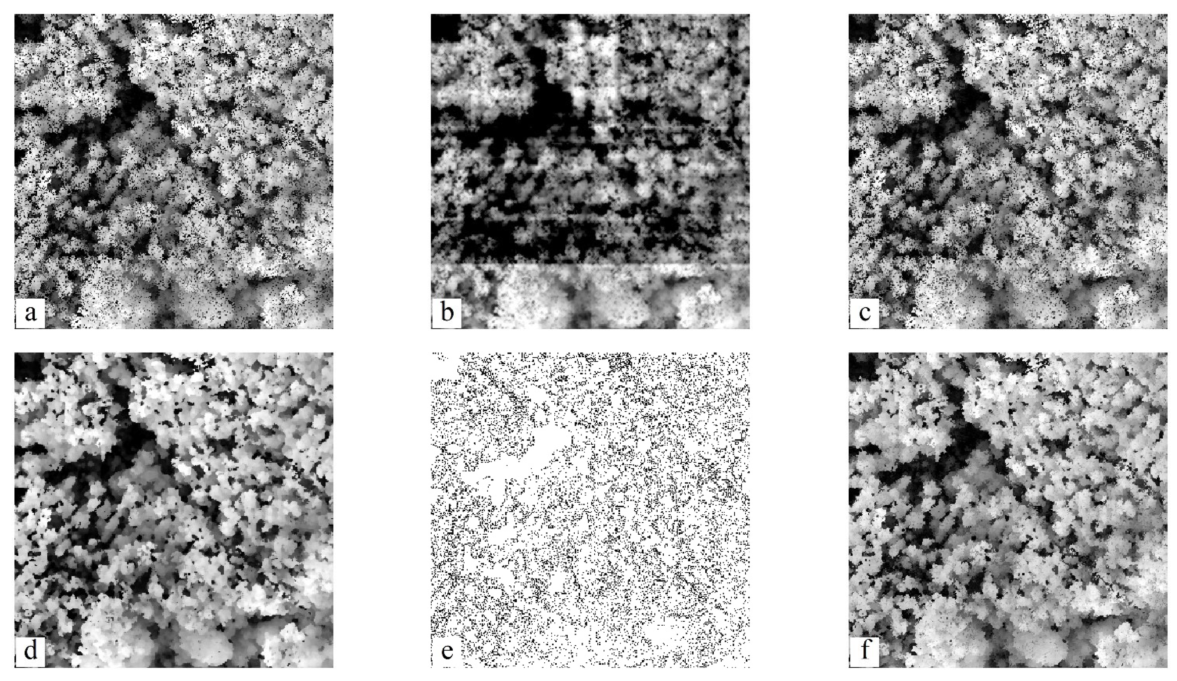
3.1. Single Wood Extraction

Canopy height model (Canopy Height Model, CHM)-based single wood segmentation is currently the most common method of obtaining information parameters for single wood in forests. In this study, a digital surface model (DSM) and a digital elevation model (DEM) obtained through data pre-processing were subtracted to generate a canopy height model (CHM), which was then used for single wood extraction.

The tree in the CHM image shows the canopy morphology as a circular, highly illuminated patch. The central brightness value of this patch is greater than the surrounding area and a distinct edge appears around it; thus, the basic shape of the canopy can be observed in the image. As LiDAR data are acquired in a row-by-row and column-by-column scan format, some black holes appear in the generated CHM, and the canopy edges will show abrupt changes in grey values on the CHM images, which are generally referred to as pits or invalid values. These abnormal crater pixels are lower than the surrounding normal pixels [14]. In order not to affect the accuracy of subsequent single-wood extraction, the original CHM needs to be dimple removed and optimised in advance. In this study, a combination of smoothing filtering and morphological opening and closing operations was used to fill the original crater region using the filtered CHM to form an optimised CHM. In order to select the most suitable filtering algorithm, three types of filtering, namely median filtering, low-pass filtering and Gaussian filtering, were compared and analysed in order to achieve the best results for CHM optimisation.

Based on the above optimised CHM, this study performed single wood extraction from the study area by the watershed segmentation algorithm. The watershed segmentation algorithm is a relatively basic mathematical morphological segmentation algorithm, the core principle of which is to transform a grey-scale image into a gradient image [15]. As shown in Figure 3, the watershed algorithm views the gradient values as a mountain, and considers each identified local minima and its adjacent area as a catchment basin. Assuming the presence of standing water in the basin, the water keeps increasing, the water level rises, and the areas with low gradients will be flooded, and when the process of water spilling out stops, the segmentation line will be formed and the image will be divided into several regions. Applying this idea to forests, the catchment basin is the forest canopy, and the dividing line is the watershed that distinguishes the canopy [16]. The watershed algorithm requires setting the minimum judgement value of tree height, Gaussian smoothing factor and radius parameters. Referring to previous studies, the minimum tree height was set to 2 m in this study, and trees of 2 m and above were used as the extracted objects; the smoothing factor was set to 1 and the smoothing radius to 5 pixels to alleviate the over-segmentation phenomenon.

In this study, the results of the extraction of single trees in the study area were classified using the obtained second-transformation stand structure data and the manually identified and decoded single tree species information of the forest, and a database of Eucalyptus single trees and Eucalyptus single tree information was obtained.

3.2. Biomass Estimation

3.2.1. Variable Filtering

Based on the extraction results of the single wood of Eucalyptus globulus, this study selected the orthophoto RGB raw band spectral features, mean, variance, homogeneity, contrast, dissimilarity, entropy, second moment, correlation based on the grey level co-occurrence matrix (GLCM), and the tree height and crown width information extracted from single wood segmentation as feature factors [17]. Terrain features are also common variables for forest biomass estimation. To improve accuracy, this study supplemented the vegetation cover (VFC), DEM, slope and aspect generated from LiDAR point cloud data with a total of 32 factors as independent variables for the construction of the Eucalyptus biomass model.

This study used the random forest algorithm for optimal variable selection for modelling Eucalyptus biomass. Random forest is a common algorithm in machine learning algorithms and is based on categorical regression trees. In random forest for decision tree construction, variables are ranked for importance, which is the basis for variable selection. There are 2 ways to rank the importance of variables in the random forest, based on the increase in OOB misclassification rate, and based on the decrease in GINI at split. The increase in OOB misclassification rate can be calculated using out-of-bag samples that are not involved in training when interpreting the model error situation [18], as follows;

$${\mathrm{OOB}}_{\mathrm{error}}=\frac{1}{\mathrm{n}}{\displaystyle \sum }_{\mathrm{i}=1}^{\mathrm{n}}{\left({\mathrm{y}}_{\mathrm{i}}-\widehat{{\mathrm{y}}_{\mathrm{i}}}\right)}^2$$

(3)

where, n is the total number of out-of-bag samples, ${\mathrm{y}}_{\mathrm{i}}$ is the measured value, $\widehat{{\mathrm{y}}_{\mathrm{i}}}$ is the model predicted value.

A random forest is based on the splitting of a node to form each tree, and the splitting of this node is based on the reduction of the GINI coefficient before and after the split [19]. The random forest gives the importance of the variables in terms of the mean value of the GINI coefficients. The random forest algorithm uses the importance () function, and the IncMSE and IncNodePurity given by the importance () function are the equivalents of these two metrics. IncMS is the root mean square error, which is equivalent to the increase in OOB misclassification rate, and IncNodePurity represents node purity, which is equivalent to the GINI coefficient. Both IncMSE and IncNodePurity are values where a higher value indicates that the corresponding variable is more important, and this study conducted variable screening based on IncMSE and IncNodePurity metrics.

3.2.2. Multiple Stepwise Regression Method

The principle of the multiple linear regression method is to establish some linear relationship between the target variables and the selected characteristic variables, and is a very practical and widely used algorithm with the following functional representation.

$${\mathrm{y}=\mathrm{w}}_1{\mathrm{x}}_1{+\mathrm{w}}_2{\mathrm{x}}_2{+\mathrm{w}}_3{\mathrm{x}}_3{+\dots +\mathrm{w}}_{\mathrm{n}}{\mathrm{x}}_{\mathrm{n}}+\mathrm{b}$$

(4)

where, $\mathrm{y}$ is the dependent variable, ${\mathrm{x}}_{\mathrm{n}}$ is the independent variable, ${\mathrm{w}}_{\mathrm{n}}$ is the model parameter, and $\mathrm{b}$ is the model constant term.

Once the multiple linear regression model is established, the significance of the selected variables on the target variable needs to be analysed so that the importance of each variable on the target variable can be evaluated. The degree of model fit is judged by the coefficients of the selected indicators. Commonly used tests for multiple regression are hypothesis testing of the established regression equation and hypothesis testing of the regression coefficients. The analysis of variance and t-test results are usually output in the equation model after multiple regression analysis, where the partial regression coefficients, standard errors and p-values are used as indicators for model testing.

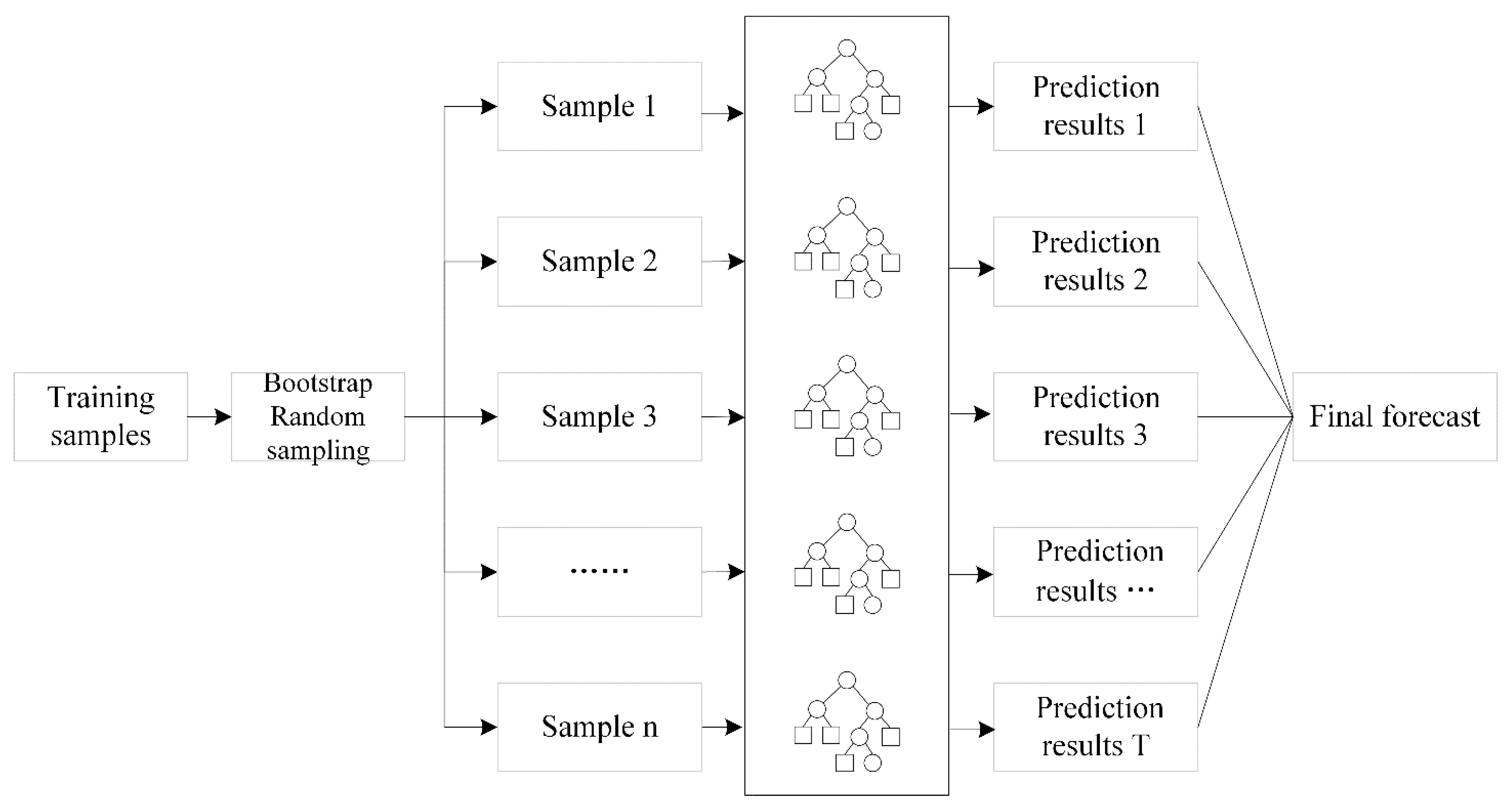
3.2.3. Random Forest Algorithm

The Random Forest algorithm is a statistical learning method based on decision trees, the core of which is the random sampling of samples, mainly through the Bootstrap method of sample processing [20]; the specific detailed process is shown in Figure 4. The random forest predictive value output model is shown in Equation (5).

$$\overline{{\mathrm{h}}_{\left(\mathrm{x}\right)}}=\frac{1}{\mathrm{N}}{{\displaystyle \sum }}_{\mathrm{t}=1}^{\mathrm{T}}\left\{\mathrm{h}\left({\mathrm{x},\mathsf{\theta }}_{\mathrm{t}}\right)\right\}$$

(5)

where $\overline{{\mathrm{h}}_{\left(\mathrm{x}\right)}}$ is the predicted value of the model’s target variable, $\mathrm{h}\left({\mathrm{x},\mathsf{\theta }}_{\mathrm{t}}\right)$ is the output based on the variables x and ${\mathsf{\theta }}_{\mathrm{t}}$, x is the filtered significant variable, ${\mathsf{\theta }}_{\mathrm{t}}$ is an identically distributed independent random variable, and N is the number of regression decision trees.

In this study, during the random forest regression modelling process, the measured Eucalyptus biomass data were divided into training data and test data in the ratio of 7:3, with 140 sets of training data and 60 sets of test data. The training data were used to fit the biomass random forest model and the test data were used to test the fitted model, which was used to evaluate the performance of the model.

The more important model parameters in the random forest regression algorithm are the number of ntree for the base learner and the number of variables to divide the subset of attributes into mtry. The grid filtering of ntree and mtry demonstrated that the number of counts was essentially constant above 600, fluctuating a little until 400, and levelling off after 400. Therefore, the optimal parameters for this study were 400 for ntree and 11 for mtry, with guaranteed performance.

3.2.4. Support Vector Machines

Support Vector Regress (SVM) is a non-parametric model that can be used to solve classification as well as regression problems in a similar way to supervised learning [21]. The use of support vector machines for solving regression problems started with the introduction of an insensitive loss function to the traditional support vector machine function. This extended the SVM, which was originally used to solve classification problems, to the regression domain, resulting in the regression type support vector machine.

The support vector machine algorithm consists of 2 steps: the first step is to construct the optimal hyperplane in the feature that can correctly partition the sample data set, and then partition the sample; the second step is to transform the sample data of the low-dimensional data to the high-dimensional space using the non-linear kernel function, so as to solve the complex calculation, the core and key is to find and construct the optimal hyperplane.

The error function most commonly used in traditional support vector machine algorithms is the least-squared sum error function [22]. In support vector machines used to solve regression analysis problems, with the introduction of an insensitive error function, we commonly use the minimax regularisation error function.

$$\mathrm{C}{\displaystyle \sum }_{n=1}^N\left({\epsilon }_n-\widetilde{{\epsilon }_n}\right)+\frac{1}{2}{w}^2$$

(6)

where C is the positive regularisation factor, n = 1,2,3…N, N is the total number of samples, w is the normal vector of the hyperplane division line, and ${\epsilon }_{\mathrm{n}}$ is the relaxation variable.

The above formula shows that the important parameters of support vector regression are C and ε. The size of the parameter C determines the penalty on the sample and the fit of the model, the smaller the value of C, the larger the error shown by the model and the overfitting will occur. ε is an insensitive parameter, representing the accuracy and computation, the smaller the ε, the better the accuracy of the regression model built by the support vector machine [23]. In this study, parameter selection was carried out through several iterations of regression modelling, and a linear kernel function with a penalty coefficient C of 1 and an ε parameter of 0.09 was finally used to model the regression of Eucalyptus biomass samples.

3.2.5. Decision Trees

Decision trees are the basic classification and regression methods in machine learning, and accordingly, there are also regression trees for prediction and regression trees for classification [24]. The internal structure of a decision tree is actually similar to a binary tree, with a single root node at the top, which contains the most information, and decreasing information from the root node down to the numerator and leaf nodes. A random forest is based on a decision tree, but unlike a random forest, a decision tree is built directly from the tree that contains the most information, the predictions are made based on this tree, and then the results are tested immediately without comparing multiple trees.

The main process of the decision tree algorithm is to first perform feature selection, build a decision tree based on the selected features, and after the final model of the decision tree has been built, to avoid errors and overfitting situations, decision tree pruning, also known as pre-pruning and post-pruning operations, is performed. When the addition of a node causes a change in regression accuracy by an amount less than a cp times the change in tree complexity, this node is considered to have to be pruned. Therefore, the cp (complexity parameter) parameter for optimal pruning needs to be set in the decision tree pruning process, and this study selected by the cross-validation error, xerror. When the xerror is smallest, the corresponding generated cp value is the best pruning cp value. This study, after several experiments, determined 0.1 as the nearest pruning cp value, as shown in Figure 5.

Decision trees are used to solve regression problems mainly by using the CART (classification and regression tree) algorithm, which firstly performs supervised clustering on the training sample data, completes the interval partitioning of the training sample, obtains the feature range of each cluster in the interval, and then finds the best features and feature values in the sample, so that the feature value has the smallest loss function. The best segmentation point is the best segmentation point, and a binomial tree is constructed. Each binomial tree is judged to split the data, and the above operation is repeated until the sample data is split, and the algorithm stops [25]. During prediction, the binary tree (the process of determining the region) will be traversed based on the characteristics of the training data samples provided, where the values of the leaf nodes are the predicted values, and each node of each binary tree will be given a predicted value, which will eventually form the predicted value of this decision tree based on the mean value, which is the predicted value of the target sample.

3.3. Accuracy Evaluation

In order to measure the comprehensive estimation level of the model, this study used the coefficient of determination R² and the root mean square error RMSE to evaluate the prediction accuracy of the model. The formulae are as follows:

$$R^2=1-\frac{\left({{\displaystyle \sum }}_{i=1}^n{\left(\widehat{y_i}-y_i\right)}^2\right)/n}{\left({{\displaystyle \sum }}_{i=1}^n{\left(y_i-\overline{y_i}\right)}^2\right)/n}$$

(7)

$$RMSE=\sqrt{\frac{1}{n}\times {\displaystyle \sum }_{i=1}^n{\left(y_i-\widehat{y_i}\right)}^2}$$

(8)

where $y_i$ is the measured value of the sample, $\widehat{y_i}$ is the predicted value of the model, n is the total number of samples.

R² indicates the error between the estimated and actual results of the target parameter. The smaller the value of R², the less accurate the model built is in representing the target, and the closer R² is to 1, the more accurate it is. RMSE indicates the distance between the target estimate and the actual result, and is the preferred performance measure when performing regression. The smaller the value of the RMSE, the better the fit of the model.

4. Results and Analysis

4.1. Single Wood Extraction Results

In this study, the CHM data were smoothed using the most classical 3 × 3 convolution window, and the obtained results were compared with the original CHM (Figure 6a–d). It could be observed that the unprocessed CHM image had many small black dots and holes, and the canopy morphology had been damaged. The CHM image after low-pass filtering was smooth, the small black holes in the image were well removed, and the overall canopy shape was well displayed, but there were large black shadows in the image, and the canopy was identified. After Gaussian low-pass filtering, many small black holes that originally existed still existed, that was, invalid values still existed, the contrast before and after the change was not obvious, and the smoothing effect was poor. After median filtering, the black holes were well removed and the overall smoothing effect was good, although some of the canopy morphology was damaged in the image. Therefore, this study used median filtered data to fill the region of invalid values for CHM optimisation (Figure 6f).

Based on the optimised CHM watershed segmentation algorithm, the single wood tree vertices were extracted from the study area and output as vector points, which were superimposed on the obtained DOM images of the study area, as shown in Figure 7. Based on the optimised CHM watershed segmentation algorithm, 4533 single trees were identified and compared with the manually identified and decoded single tree species information for this forest site, 1741 undetected but actually present single trees were found and 963 were mis-segmented, with an accuracy of 77%. This study area has dense vegetation, high densities, overlapping tree canopies and a large area, so the overall identification accuracy of the single wood segmentation method was slightly lower than in the lower density areas. Based on the manually identified and decoded information on single wood species in this forest, this study obtained the single wood results of Eucalyptus in the study area (Figure 8).

4.2. Biomass Estimation Results

After experimentation, this study chose to base the variable selection on the importance given by the IncNodePurity indication value. Ultimately, a total of 10 variables were selected (Figure 9), namely: DEM, Slope, Aspect, CD, $r_{mean}$, $b_{mean},b_{cor}, \mathrm{VFC},r_{DN}$, $b_{DN}.$

The multiple regression model based on the filtered factors was

$$\begin{gathered} \mathrm{AGB}=2.0418r_{mean}-2.8189b_{mean}-0.0095b_{dis}-0.2651\mathrm{DEM}+0.5486 \\ \mathrm{VFC}+25.1370\mathrm{Slope} \end{gathered}$$

Since machine learning algorithms are similar to black box operations, the “model” in the algorithm was the output of each algorithm running on the data; thus, the random forest model, support vector machine model and decision tree model built from the factors filtered by the random forest algorithm do not have specific model coefficients.

In order to build and validate the Eucalyptus biomass model, the collected Eucalyptus sample data were randomly divided into a training set and a test set in the ratio of 7:3 in this study. In order to obtain more stable results, the results of the different models were validated using the ten-fold cross-validation method and the fit performance of the obtained models on the training and test sets were compared (Figure 10).

In Figure 10, the red line showed the fit between the Eucalyptus biomass predicted by each model and the sample measured Eucalyptus biomass, with the accuracy of each model labelled next to it. On the training set (Figure 10a–d), the accuracy of the four Eucalyptus biomass models performed as RF > SVR > CART > MLR. It could be observed that the RF model performed the best in the training set with the R² of 0.9375 and the RMSE of 9.8024; followed by the SVR model with the R² of 0.7173 and the RMSE of 14.1331; the decision tree model ranked third with the R² of 0.5722 and the RMSE of 16.7032; the multiple linear regression model was the worst fit with the R² of 0.4132 and the RMSE of 19.4161. The smaller the value of the coefficient of determination R², the lower the degree of model fit, and the closer the coefficient of determination R² is to 1, the better the fit of the model and the higher the model accuracy. The smaller the value of the root mean square error RMSE, the better the fit of the model. The results of these two metrics demonstrated that the RF model had the highest overall accuracy on the training data; overall, all three approaches to machine learning built models with higher accuracy than the linear regression model.

To further test the accuracy of the established Eucalyptus biomass estimation model, model accuracy tests were conducted on the screened test set (Figure 10e–h). The RF model also performed well on the test set, with a coefficient of determination R² of 0.7855 and a root mean square error RMSE of 13.0377. The SVR model performed second best, with a coefficient of determination R² of 0.4822 and a root mean square error RMSE of 17.1953. Multiple regression model number three, with a coefficient of determination R² of 0.3490 and a root mean square error RMSE of 20.2352. The decision tree model was the least effective, with a coefficient of determination R² of 0.2856 and a root mean square error RMSE of 22.3906.

In order to provide a more visual representation of the fitting results of each model, the accuracy of the fit of each model was summarised in this study (

Table 3. Summary of biomass estimation accuracy.

Methods	Training Set		Test Set
	R2	RMSE	R2	RMSE
MLR	0.4132	19.4161	0.3490	20.2352
RF	0.9375	9.8024	0.7855	13.0377
SVR	0.7173	14.1331	0.4822	17.1953
CART	0.5722	16.7032	0.2856	22.3906

). As can be observed from Table 3, the multiple regression models had low overall accuracy and did not fit particularly well across multiple characteristics and complex variables. In contrast, the machine learning method, RF, which had the highest accuracy, performed better in fitting predictions and was more able to combine the important features of each variable. This is an advantage of the RF algorithm, where the input variables do not need to be normalised and the characteristics of the variables can be analysed and processed in an integrated manner. Relatively speaking, the decision tree had the lowest accuracy on the test set. This study compared the predicted values of the decision tree for the sample with the measured values and found that the decision tree model was overfitted to some extent, with the overall prediction of the data being high and poorly fitted. Overall, the machine learning approach had higher prediction accuracy compared to the multiple regression model approach.

Machine learning algorithms avoid human interference factors, are computer-automated processes that only input and output results, and do not have the specific regression equations that linear regression does. Of the machine learning methods, the RF model had the highest accuracy in estimating Eucalyptus biomass, and the method was more likely to derive the importance of each variable, providing information on the significance of the relationship between the Eucalyptus biomass estimation model and each variable. Overall, both the machine learning random forest and support vector machine models achieved higher prediction accuracy than the multiple regression model approach, indicating that the machine learning algorithms were able to estimate Eucalyptus above-ground biomass more accurately and were more suitable for building Eucalyptus biomass estimation models in this study area. Based on the accuracy tests and comparative analysis of the four models, the RF algorithm was used to predict the biomass of Eucalyptus trees in the whole study area, and Eucalyptus biomass mapping was carried out in the study area based on the obtained Eucalyptus biomass predictions.

5. Discussions

This study compared and analysed the performance of traditional parametric models (multiple linear regression) and machine learning methods (random forests, support vector machines and decision trees) in single wood-scale biomass model building. Of the four methods, the accuracy of the non-parametric model of machine learning was clearly higher than that of the parametric model of linear regression, which reflected the advantages of machine learning algorithms. The modelling process, where the machine learning algorithm avoids human interference factors, is an automated computer process that only inputs and outputs results and does not have a specific regression equation as linear regression does. Of the machine learning methods, the RF model had the highest accuracy in estimating Eucalyptus biomass, and the method could moreover derive the importance of each variable, providing information on the significance of the relationship between the Eucalyptus biomass estimation model and each variable. In comparison with other biomass estimation methods, the accuracy of Eucalyptus biomass estimation in this study was high, and the spatial resolution of Eucalyptus biomass distribution reached 0.05 m, which enabled accurate prediction of the distribution details of Eucalyptus biomass in the study area and was of practical reference value. Compared with the accuracy of biomass estimation based on the same machine learning method, e.g., Li et al. constructed a forest above-ground biomass estimation model based on Landsat 8 OLI images by depression class (R² = 0.41, RMSE = 23.0 mg-hm⁻²) [26]; Xu used waveform data to invert forest leaf area index and single wood biomass estimation in (R² = 0.708, RMSE = 142.664 kg) [27]; Liu estimated the above-ground biomass of single wood in Changbai Larch plantation in Changbai Mountain area (R² = 0.799, RMSE = 0.93 kg) [28]; Zhang estimated the above-ground biomass of single wood based on canopy height model data, combined with the biomass estimation was based on the canopy height model data combined with the measured data from the Penobscot Experimental Forest (R² = 0.90, RMSE = 54.46 kg) [13]; and the R² index and RMSE index of random forest were better in this paper.

In this study, high-precision airborne LiDAR point cloud data and multispectral data were used for Eucalyptus biomass estimation. Although the estimation accuracy is high, there are still some issues to be further investigated.

(1)

In terms of single wood segmentation in dense vegetation cover areas, how to determine whether there are small trees below the dense canopy and how to identify and segment these small trees are issues that need to be studied in depth in the next step. The further inclusion of data sources, such as ground-based radar data, on top of fused data can be considered in order to obtain more information on tree structure and location, and thus improve the accuracy of the Eucalyptus biomass estimation model.

(2)

Data such as tree age and storage volume were not used in this study, and further consideration can be given to adding data such as the age of Eucalyptus trees and the storage volume of the area in which they are located in subsequent studies to further improve the accuracy of biomass modelling.

(3)

The combination of multi-source data and machine learning algorithms can provide accurate and rapid biomass measurements at the single-wood scale, which can provide more accurate information for the management of regional biomass resources statistics. Deep learning algorithms may also be considered in the future to explore the performance of different algorithms for biomass estimation of eucalypts over large areas.

6. Conclusions

This study combined airborne LiDAR point cloud data and aerial orthophotos to develop a model for estimating the biomass of Eucalyptus plantations in the Zengcheng forestry site in Guangzhou, combining forestry resources type II survey stand data and Eucalyptus sample data. Firstly, the study extracted single trees from the study area based on the optimised CHM Watershed Segmentation algorithm, and then obtained the segmentation results of Eucalyptus trees in the study area. Based on the results of the Eucalyptus stand segmentation, a multiple linear regression method within the parametric model and a non-parametric random forest, support vector machine and decision tree algorithm were used to build a biomass estimation model for the Eucalyptus trees in the study area, and the performance of the four methods in Eucalyptus biomass estimation was compared and validated for accuracy to determine the best Eucalyptus biomass estimation model. The main conclusions obtained from this study were as follows.

In areas with dense vegetation, high densities and overlapping tree canopies, the optimised CHM watershed segmentation algorithm could effectively achieve a large area extraction of single trees with an accuracy of 77% for single tree segmentation.

The accuracy of the models built by all three methods of machine learning was higher than that of the linear regression model, and of the machine learning models, the RF model had the highest overall accuracy on the training data. On the training set, the RF model performed the best (R² = 0.9375, RMSE = 9.8024); the SVR model was the second best (R² = 0.7173, RMSE = 14.1331); on the test set, the RF model also performed the best (R² = 0.7855, RMSE = 13.0377); the SVR model was the second best (R² = 0.4822, RMSE = 17.1953). RMSE = 17.1953. Overall, the RF algorithm was more suitable for predicting the biomass of eucalypts.

References

1. Hyypp, J.; Kelle, O.; Lehikoinen, M.; Inkinen, M. A segmentation-based method to retrieve stem volume estimates from 3-D tree height models produced by laser scanners. IEEE Trans. Geosci. Remote Sens. 2001, 39, 969–975. [Google Scholar] [CrossRef]
2. Fang, J.; Chen, A.; Peng, C.; Zhao, S.; Ci, L. Changes in Forest Biomass Carbon Storage in China Between 1949 and 1998. Science 2001, 292, 2320–2322. [Google Scholar] [CrossRef]
3. Yu, X.X.; Lu, S.W.; Jin, F.; Chen, L.H.; Rao, L.Y.; Lu, G.Q. The assessment of the forest ecosystem services evaluation in China. Acta Ecol. Sin. 2005, 25, 2096–2102. [Google Scholar]
4. Li, H.K.; Lei, Y.C.; Zeng, W.S. Forest carbon storage in China estimated using forestry inventory data. Sci. Silvae Sin. 2011, 47, 7–12. [Google Scholar]
5. Li, D.R.; Wang, C.W.; Hu, M.Y.; Liu, S.G. Research progress in estimating forest biomass by remote sensing technology. Geomat. Inf. Sci. Wuhan Univ. 2012, 37, 631–635. [Google Scholar]
6. Jiao, Y.; Hu, H.Q. Carbon storage and its dynamics of forest vegetations in Heilongjiang Province. Chin. J. Appl. Ecol. 2005, 16, 2248–2252. [Google Scholar]
7. Zhang, L.Q. Research on Remote Sensing Biomass Estimate of Eucalyptus Plantation; Guangxi University: Nanning, China, 2012. [Google Scholar]
8. Thomas, V.; Treitz, P.; Mccaughey, J.H.; Morrison, I. Mapping stand-level forest biophysical variables for a mixedwood boreal forest using lidar: An examination of scanning density. Can. J. For. Res. 2006, 36, 34–47. [Google Scholar] [CrossRef]
9. Zheng, H.M. Compatible Models of Individual Tree Biomass Factors for Simao Pine Natural Forest; Southwest Forestry University: Kunming, China, 2015. [Google Scholar]
10. Ou, J.D.; Ou, J.L.; Kang, Y.W. Single tree biomass simulation of taxus yunnanensis plantation based on crown morphological index. J. Southwest For. Univ. Nat. Sci. 2022, 42, 1–9. [Google Scholar]
11. Gleason, C.J.; Im, J. Forest biomass estimation from airborne LiDAR data using machine learning approaches. Remote Sens. Environ. 2012, 125, 80–91. [Google Scholar] [CrossRef]
12. Li, D. Retrieval and Estimation Research of Forest Parameters Based on Digital Aerial Photograph Data; Institute of Remote Sensing and Digital Earth Chinese Academy of Sciences: Beijing, China, 2018. [Google Scholar]
13. Zhang, P.; Ma, Q.X.; Lv, J.; Ji, J.L.; Li, Z.W. Application of machine learning algorithms in estimation of aboveground biomass of forest. Bull. Surv. Mapp. 2021, 28–32. [Google Scholar] [CrossRef]
14. Wang, Y.F.; Yue, T.X.; Zhao, M.W.; Du, Z.P.; Liu, X.F.; Liu, S.; Song, E.F.; Sun, W.Z.; Zhang, Y.L. Study of factors impacting the tree height extraction based on airborne LIDAR data. J. Geo-Inf. Sci. 2014, 16, 958–964. [Google Scholar]
15. Zhang, H.Q. Research on Single Wood Segmentation and Tree Height Estimation Method Based on UAV LiDAR; Kunming University of Science and Technology: Kunming, China, 2021. [Google Scholar]
16. Jin, Z.M.; Cao, S.S.; Wang, L.; Sun, W. A method for individual tree-crown extraction from USA remote sensing image based on U-Net and watershed algorithm. J. Northwest For. Univ. 2020, 35, 194–204. [Google Scholar]
17. Ding, J.Q.; Huang, W.L.; Liu, Y.C.; Hu, Y. Estimation of forest aboveground biomass in northwest hunan province based on machine learning and multi-source data. Sci. Silvae Sin. 2021, 57, 36–48. [Google Scholar]
18. Cho, A. High density biomass estimation for wetland vegetation using WorldView-2 imagery and random forest regression algorithm. Int. J. Appl. Earth Obs. 2012, 18, 399–406. [Google Scholar]
19. Wang, Y.F.; Pang, Y.; Shu, Q.T.; University, S.F. Counter-estimation on aboveground biomass of hevea brasiliensis plantation by remote sensing with random forest algorithm-a case study of Jinghong. J. Southwest For. Univ. 2013, 33, 38–45. [Google Scholar]
20. You, S.B.; Yan, Y. Stepwise regression analysis and its application. Stat. Decis. 2017, 14, 31–35. [Google Scholar]
21. Vapnik, V.; Chapelle, O. Bounds on error expectation for support vector machines. Neural Comput. 2000, 12, 2013–2036. [Google Scholar] [CrossRef]
22. Ara, A.; Maia, M.; Louzada, F.; Macêdo, S. Regression random machines: An ensemble support vector regression model with free kernel choice. Expert Syst. Appl. 2022, 202, 117107. [Google Scholar] [CrossRef]
23. Gao, Y.K. Aboveground Forest Biomass Estimation Based on Machine Learning Algorithms and Multi-Source Data in a Typical Subtropical Region; Zhejiang A&F University: Hangzhou, China, 2018. [Google Scholar]
24. Karka, P.; Papadokonstantakis, S.; Kokossis, A. Environmental impact assessment of biomass process chains at early design stages using decision trees. Int. J. Life Cycle Assess. 2019, 24, 1675–1700. [Google Scholar] [CrossRef]
25. Dong, H.Z.; Xu, H.P.; Lu, B.; Yang, Q. A cart-based approach to predict nitrogen oxide concentration along urban traffic roads. Acta Sci. Circumstantiae 2019, 39, 1086–1094. [Google Scholar]
26. Li, C.; Li, Y.; Li, M. Improving forest aboveground biomass (AGB) estimation by incorporating crown density and using Landsat 8 OLI iImages of a subtropical forest in western hunan in central China. Forests 2019, 10, 104. [Google Scholar] [CrossRef] [Green Version]
27. Xu, G.C. Forest LAI and individual trees biomass estimation using small-footprint fyll-waveform LiDAR data. Chin. Acad. For. Sci. 2013. Available online: https://kns.cnki.net/KCMS/detail/detail.aspx?dbname=CDFD1214&filename=1013378640.nh (accessed on 14 June 2022).
28. Liu, F.; Tan, C.; Zhang, G.; Liu, J.X. Estimation of forest parameter and biomass for individual pine trees using airborne LiDAR. Trans. Chin. Soc. Agric. Mach. 2013, 44, 219–224. [Google Scholar]
Figure 1. Location and digital orthophoto map of research area.
Sustainability 14 10576 g001
Figure 2. Eucalyptus sample.
Sustainability 14 10576 g002
Figure 3. Schematic diagram of watershed segmentation algorithm.
Sustainability 14 10576 g003
Figure 4. Schematic diagram of random forest.
Sustainability 14 10576 g004
Figure 5. Best pruning cp value.
Sustainability 14 10576 g005
Figure 6. The optimisation process of CHM. (a) raw images; (b) low pass filtering; (c) gaussian law pass filtering; (d) median filtering; (e) invalid value; (f) optimised CHM.
Sustainability 14 10576 g006
Figure 7. Single tree point extraction based on CHM model.
Sustainability 14 10576 g007
Figure 8. The range of Eucalyptus.
Sustainability 14 10576 g008
Figure 9. Factor importance by random forest. (a) %IncMSE; (b) IncNodePurity.
Sustainability 14 10576 g009
Figure 10. Performance of different model on training sets (ad) and test sets (eh).
Sustainability 14 10576 g010aSustainability 14 10576 g010b