Identifying the Real Income Disparity in Prefecture-Level Cities in China: Measurement of Subnational Purchasing Power Parity Based on the Stochastic Approach

Abstract

Common prosperity has become the consensus of the times on development. This study aims to establish a generalized framework of the multilateral index number system under the stochastic approach and further derive the Geary–Khamis (GK) system and the Rao system under the stochastic approach to measure subnational Purchasing Power Parities (PPPs) for quantifying the real income disparity, excluding the effect of prices in prefecture-level cities in China, accurately. The results reveal that: (1) The GK system and the Rao system under the stochastic approach have advantages in addressing information loss and reliability measures, and further improve the spatial price index theory; (2) The distribution of price levels in China is in line with the trend of decreasing economic levels from east to west, which may be related to the Penn effect; (3) Compared with nominal income, real income increased significantly, and the ratio of the highest to the lowest real income in China decreased from 2.62 to 2.02. Real income, excluding the effect of prices, shows a new characteristic of moving toward the north for the high-income agglomeration areas and toward the southwest for the low-income agglomeration areas. These findings are conducive to the adoption of regionally differentiated measures to promote the realization of common prosperity, which has significant practical relevance.

1. Introduction

Common prosperity has become the consensus of the times on development. To fulfill common prosperity, the first thing is to develop the social economy to achieve “prosperity”, but the key is to narrow the gap to achieve “common” [1]. However, how large is the income disparity between regions in China? This question has not been agreed upon in the academic community. Due to differences in economic development, resource endowment, location advantages, consumption habits, and many other factors, there are objective differences in price levels between different prefecture-level cities in China, and the same income cannot buy the same amount of goods and services in different cities, resulting in nominal indicators such as per capita income not truly reflecting living standards and the real income disparity [2,3,4]. For example, east coastal areas have reached the level of developed countries, while the living standards of the central and western regions are just above the poverty line [5]. Therefore, real income is a better measure of welfare than nominal income, and subnational Purchasing Power Parities (PPPs) provide a “bridge” [6].

The International Comparison Program (ICP), sponsored by the United Nations Statistical Commission and organized by the World Bank, gives an indicator to quantify the level of price differences between economies’ PPPs. Empowered by the PPPs, it offers the possibility to quantify the price level and real income disparity between regions. However, the methodology of purchasing power parity (PPP) originating from the Organisation for Economic Co-operation and Development (OECD) is more suitable for marketized and highly homogeneous economies [7,8]. Thus, the prices of some commodities cannot well reflect their real price levels in China due to imperfect marketized development. There is a lack of a statistical index to measure the reliability of the results in order to provide an objective basis for pre-selection and post-improvement of the methodology used. Therefore, it is crucial to find a scientific and objective method to measure price levels between prefecture-level cities in China, and, furthermore, to accurately quantify the real income disparity between prefecture-level cities in China, excluding the influence of price factors so as to promote the realization of common prosperity, which has important theoretical and practical significance.

As Biggeri et al. pointed out, comparisons of income and welfare generally imply two aspects, namely, an adjustment of nominal income for price changes over time and an adjustment of price differences across space [9]. Theoretical discussion and statistical practice of the adjustment of nominal income for price changes over time are always paid much more attention [10,11,12,13,14]. However, the research on the adjustment of price differences across space is ignored either intentionally or unintentionally [15]. The importance of the research on subnational PPPs has been emphasized in countries characterized by large territorial differences in consumer preferences, as well as in the quality of products and household characteristics [16,17,18], and there has been a burgeoning interest in calculating subnational PPPs in large countries, such as India [19], the United States [20], and China [15], as well as in smaller countries such as the United Kingdom [21] and Italy [22]. In order to obtain a more accurate result of the price and income disparity in China, Jiang and Li first introduced subnational PPPs into the research in China [23]. However, the methodology used in this study does not have the characteristics of the spatial index. Biggeri et al. introduced the Gini–Éltető–Köves–Szulc (GEKS) approach to measure the subnational PPPs in China [24]. Further, Chen measured the subnational PPPs across different provincial areas in China according to the framework of the ICP methodology [25]. However, due to the difficulty of obtaining price data, there is a lack of research on the measurement of PPPs and the quantification of real income in prefecture-level cities in China.

The above-mentioned studies on subnational PPPs in China have the problem that the degree of reliability of the measurement results cannot be measured due to the limitation of the PPP measurement method. In addition, research on the measurement of subnational PPPs in China mostly uses index methods, such as GEKS and Geary–Khamis (GK), which are sensitive to missing values and cannot effectively fill in the missing values, resulting in information loss. Stochastic approaches have significant advantages in terms of measuring the reliability of results and filling in missing values, and it is an important issue to randomize the index method and explore the corresponding level of reliability. Based on stochastic ideas, Summers proposed a regression method for measuring PPPs, the Country–Product–Dummy (CPD) method, which to a certain extent compensates for the shortcomings of the index method [26]. However, the CPD method cannot be used for the measurement of PPPs above the basic heading level. Selvanathan and Rao attempted to randomize the Törnqvist method, the GEKS method, and the GK method, which can be used in the basic heading level, and proposed a conditional stochastic approach to measure the standard error of the exponential method, taking research on the stochastic approach to a new level [27]. Further, Diewert completed the existing stochastic approach by creating a different form of the law of one price giving the GK, the Iklé exponential method of randomization [28]. In order to relax the restriction of making strict prerequisite assumptions on the data distribution, the generalized method of moments (GMM) method for this problem was introduced to estimate the unknown parameters, which overcomes the problem that the prerequisite assumptions are difficult to satisfy to some extent [29,30].

The contribution of this paper is shown below. With the aim of improving the existing methodology used in the research on subnational PPPs in China, we introduce the stochastic approach proposed by Rao and Hajargasht [29] and develop a generalized framework for the multilateral comparative index system under the stochastic approach. There are two advantages of this framework. Firstly, it provides a set of equations to measure subnational PPPs by a bottom-up approach, which can be used regardless of the completeness or absence of price data, making use of the available price information to improve the estimation accuracy as far as possible; Secondly, it introduces heteroskedasticity, robust standard errors to measure the degree of reliability of the measurement results, so that the corresponding reliability indicators can be obtained while measuring subnational PPPs.

Another contribution of the paper is measuring subnational PPPs in China at the prefectural city level, compared to most existing studies that only analyze subnational PPPs at the provincial level in China, where commodity prices in provinces are mostly collected in the more developed provincial capitals and are not representative of the general level of the province [15,24]. Therefore, the findings of this paper are more general and the sample size of the city-level measurement study is larger, making it more suitable for further research. Meanwhile, in terms of the data used, the paper selects more than 10,000 price collection points in 76 prefecture-level cities in China, collects data on the prices of 232 specification commodities, and assesses the quality of the data in an attempt to ensure that survey price levels better reflect the actual situation in China, and thus measures subnational PPPs and analyzes the real income disparities in 76 prefecture-level cities in China. The result indicates that the improved PPP measurement method is more accurate and robust, and meanwhile, the income disparity between prefecture-level cities in China is not as large as the nominal data indicate, and the real income between prefecture-level cities in China shows new distribution characteristics.

The remainder of the paper is laid out as follows. Section 2 presents the multilateral comparative index system under the stochastic approach for estimating subnational PPPs in China. Section 3 describes the dataset used in our empirical analyses. Section 4 reports the estimation results, explores the applicability of the methodology, and analyzes real income disparities in prefecture-level cities in China. Finally, conclusions, limitations, and some possible further developments are drawn in the last section.

2. Methodology

Influenced by many factors such as resource endowment, location advantage, and consumption habits, there are objective differences in price levels among prefecture-level cities in China, resulting in nominal income not truly reflecting people’s real living standards and real income disparity. In order to quantify the real income level and real income disparity of prefecture-level cities in China, this paper firstly introduces PPPs to accurately measure inter-regional price differences. However, the PPP index measurement methods, such as GEKS and GK, which are mainly used around the world, are extremely sensitive to missing values, and the degree of reliability of the measurement results is difficult to measure. In order to solve the above problems, based on the existing stochastic approach, a generalized framework for the multilateral comparative index system under the stochastic approach for measuring subnational PPPs is developed by exploring different forms of law of one price and using modern econometric tools such as GMM. Based on this framework, the GK system under the stochastic approach and the Rao system under the stochastic approach can be derived.

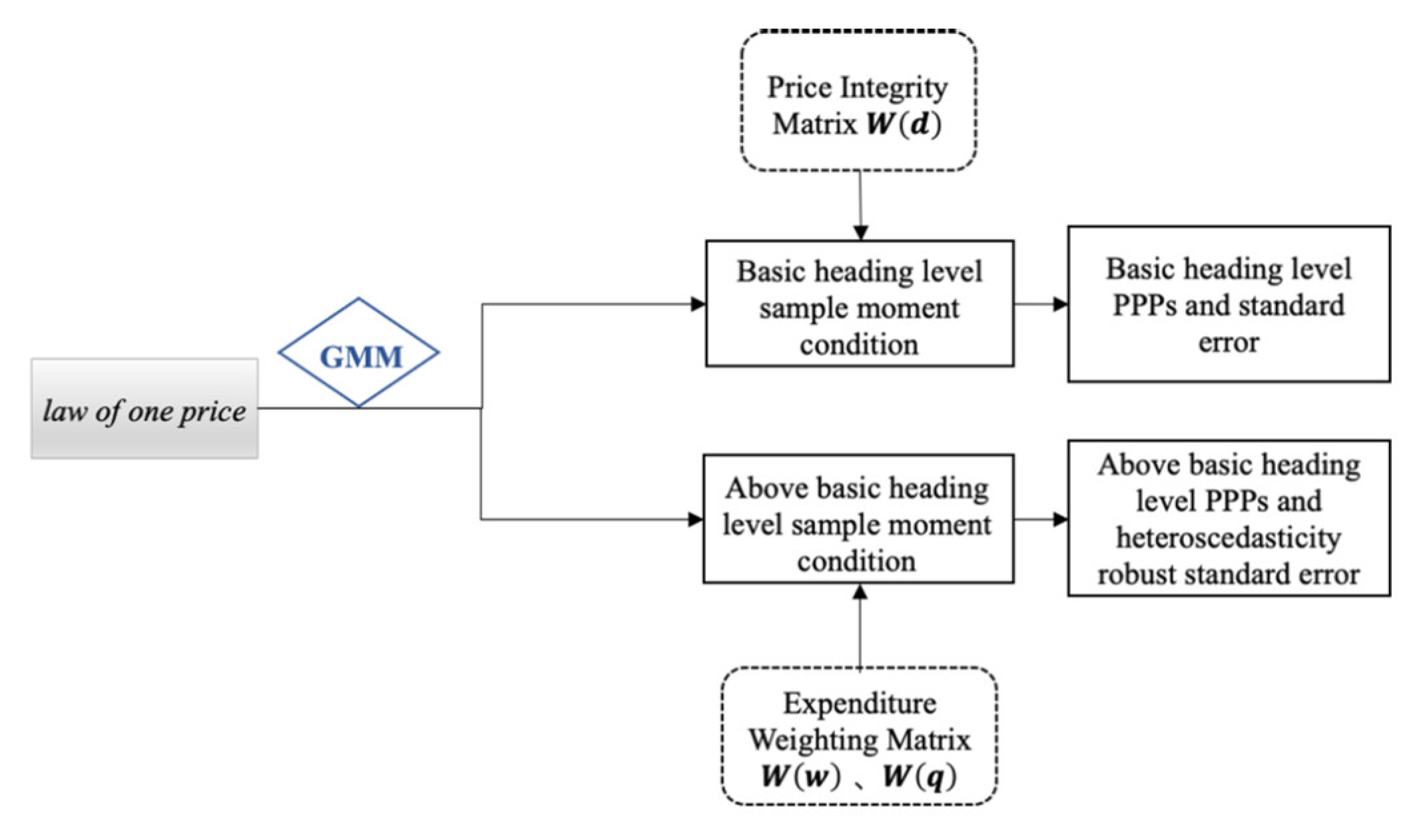
2.1. The Generalized Framework under the Stochastic Approach

To address the problems of heteroskedasticity in multi-source data and the prevalence of missing data, a stochastic methodological framework for measuring subnational PPPs is built in this paper, as shown in Figure 1. Through the generalized framework shown in Figure 1, a set of equations to measure subnational PPPs by a bottom-up approach are obtained, which can be used regardless of the completeness or absence of price data, making use of the available price information to improve the estimation accuracy as far as possible, and heteroskedasticity, robust standard errors, to measure the degree of reliability of the measurement results can also be obtained in the meanwhile.

The stochastic framework developed in this paper is based on the economic theory of the law of one price, which postulates that in the absence of trade barriers and transaction costs, each country can trade homogeneous and comparable goods at the same price level, and this law in the form of a statistical model can be expressed by:

$$p_{ij}=PP{P}_j\ast P_i\ast v_{ij}.$$

(1)

where $p_{ij}$ is the observed price of commodity i and region j, $PP{P}_j$ is the purchasing power parity of region j, $P_i$ is the average price of commodity i, and $v_{ij}$ is the random disturbance term.

The basic statistical model of the law of one price based on Equation (1) can be deformed and constructed as a corresponding linear or non-linear regression model. To relax the presupposition on the form of the distribution of the random disturbance terms, this framework uses the GMM method. The sample moment conditions at the basic heading level were constructed by introducing a price integrity matrix $\mathit{W}\left(\mathit{d}\right)$ for commodities at the basic heading level, to enable efficient filling of missing price data. The expenditure weighting matrix $\mathit{W}\left(\mathit{w}\right)$ or $\mathit{W}\left(\mathit{q}\right)$ is introduced to quantify the degree of importance of different basic headings above the basic heading level. Finally, the regional PPPs and heteroscedasticity, robust standard error, are measured. Where a diagonal matrix of order MN∗MN is denoted by $\mathit{W}\left(\mathit{d}\right)=Diag\left(d_{ij}\right)$ with $d_{ij}=1$ if commodity i is priced in region j, and $d_{ij}=1$ otherwise; $\mathit{W}\left(\mathit{w}\right)=Diag\left(w_{ij}\right)$ denotes a diagonal matrix with expenditure shares in its diagonal; $\mathit{W}\left(\mathit{q}\right)=Diag\left(q_{ij}\right)$ denotes a diagonal matrix with the number of commodities in its diagonal.

As the diversity of price data sources and the differences in the price of commodities can lead to heteroscedasticity to some extent, this framework uses a heteroscedasticity robust covariance matrix formula to optimize the estimated standard errors, and thus addresses the problem of heteroscedasticity in the random disturbance terms. This method is used for two reasons: firstly, it is more robust and more widely applicable. For example, where the specific form of the heteroscedasticity of the random disturbance term is unknown and the model is non-linear and non-additive, the heteroscedasticity cannot be removed using weighted least squares estimation. By improving the heteroscedasticity through the optimized covariance formula, subsequent hypothesis testing and interval estimation can be carried out normally; secondly, the heteroscedasticity robust covariance matrix formula can take into account the uncertainty in the measurement of the basic heading of PPPs, making it possible to measure the reliability of PPPs above the basic heading levels more accurately.

In a nutshell, adopting the generalized framework under the stochastic approach cannot only make use of the available price information to improve the estimation accuracy as far as possible, but also obtain heteroskedastic robust standard errors to measure the degree of reliability of the measurement results, so as to makes estimation results more credible.

2.2. The GK System under the Stochastic Approach

The GK method proposed by Geary is additive and suitable for a structural analysis of the economy, and has been used in the ICP [31]. This paper derives and interprets the exponential formula and the formula for the estimated standard error in the system based on the non-linear form of the law of one price, as shown in Equation (2) in the generalized framework of the multilateral index system under the stochastic approach, and improves the method for measuring the basic heading level.

$$r_{ij}=\frac{p_{ij}}{P_{i}PP{P}_j}-1.$$

(2)

2.2.1. The Basic Heading Level

Using the traditional measurement method, if price data for a commodity are missing in a particular region, price information for the corresponding commodity in all regions is discarded, resulting in a certain degree of information loss. Based on this, the basic heading level measurement method in the generalized framework is improved to make use of as much sample information as possible, and to increase the degree of reliability of the estimation results. The improved method has good applicability and can be used to derive and calculate the indices and their standard errors regardless of the presence of missing values in the price data of the commodity.

Since the model shown in Equation (2) is a non-linear and non-additive model, the GMM method is used to estimate the unknown parameters in order to obtain consistent estimates, and the specific derivation process for solving the parameters of the non-linear and non-additive model is shown in Appendix A. Based on the GMM method, the sample moment conditions shown in Equation (3) can be constructed to estimate the subnational PPPs and the average price between regions.

$$\frac{1}{{{\displaystyle \sum }}_{j=1}^M{N}_j}{\mathit{R}}_{\mathit{W}}{}^{\prime }\mathit{r}=\mathbf{0}.$$

(3)

where $N_j$ is the number of commodities priced in region j out of a total of N commodities belonging to the basic heading, and $M_i$ is the number of the regions in which commodity i is priced. ${\mathit{R}}_{\mathit{W}}{}^{\prime }={\mathit{R}}^{\prime }\mathit{W}\left(\mathit{d}\right)$; $\mathit{r}=\left\{r_{ij}\right\}$; $\mathit{R}\ne \mathit{R}{}^{\ast }=E\left(\frac{\partial \mathit{r}\left(\mathit{y},\mathit{X},\mathit{\beta }\right)}{\partial {\mathit{\beta }}^{\prime }}\left|\mathit{X}\right.\right)$. $\mathit{R}$ replaces ${\mathit{I}}_N$ in the optimal matrix ${\mathit{R}}^{\ast }$ with ${\mathit{P}}_N$, and this replacement is not arbitrary because this moment condition in weighted form can derive the GK index [30].

Based on the above moment conditions, a set of equations can be obtained, as shown in Equation (4), which can be solved by the iterative method to obtain the unknown parameters.

$$\begin{gathered} \widehat{PP{P}_j}=\frac{{{\displaystyle \sum }}_{i=1}^{N_j}{p}_{ij}}{{{\displaystyle \sum }}_{i=1}^{N_j}{\widehat{P}}_i}. \\ {\widehat{P}}_i=\frac{1}{M_i}{{\displaystyle \sum }}_{j=1}^{M_i}(\frac{p_{ij}}{\widehat{PP{P}_j}}). \end{gathered}$$

(4)

The formula for the variance of the unknown parameter estimates is shown in Equation (5):

$$Var\left(\widehat{\mathit{P}},\widehat{\mathit{P}\mathit{P}\mathit{P}}\right)={\widehat{\sigma }}^2{\left[{\widehat{\mathit{D}}}^{\prime }\widehat{\mathit{R}}\right]}^{-1}{\widehat{\mathit{R}}}^{\prime }\widehat{\mathit{R}}{\left[{\widehat{\mathit{R}}}^{\prime }\widehat{\mathit{D}}\right]}^{-1}.$$

(5)

where $\widehat{\mathit{D}}=\frac{\partial \mathit{r}\left(\mathit{y},\mathit{X},\mathit{\beta }\right)}{\partial {\mathit{\beta }}^{\prime }}{|}_{\widehat{\mathit{\beta }}}$.

It is worth noting that the set of equations shown in Equation (4) gives the same price index as the Dutot index when the price data are complete. The traditional Dutot index inevitably loses valid information in the presence of missing data, and this improvement allows the traditional index method to be optimized.

2.2.2. Above the Basic Heading Level

Above the basic heading level, weight information should be taken into account in the model. Based on the non-linear and non-additive model shown in Equation (2), a set of sample moment conditions shown in Equation (6) is constructed for the derivation of the index formula and the formula of heteroscedastic robust standard errors for the GK system under the stochastic approach.

$$\frac{1}{NM}{\mathit{R}}^{\prime }\mathit{W}\left(\mathit{q}\right)\mathit{r}=\mathbf{0}.$$

(6)

The specific form of ${\mathit{R}}^{\prime }$ in the moment condition is the same as in the case of the basic heading level of the GK system under the stochastic method.

The sample moment conditions in Equation (6) lead to the following set of equations for measuring subnational PPPs.

$$\begin{gathered} \widehat{PP{P}_j}=\frac{{{\displaystyle \sum }}_{i=1}^N{p}_{ij}{q}_{ij}}{{{\displaystyle \sum }}_{i=1}^N{\widehat{P}}_i{q}_{ij}}. \\ {\widehat{P}}_i={{\displaystyle \sum }}_{j=1}^M(\frac{p_{ij}{q}_{ij}}{\widehat{PP{P}_j}})/{{\displaystyle \sum }}_{j=1}^M{q}_{ij}. \end{gathered}$$

(7)

The covariance matrix formula for the corresponding estimated coefficients can be expressed as:

$$Var\left(\widehat{\mathit{P}},\widehat{\mathit{P}\mathit{P}\mathit{P}}\right)={\widehat{\sigma }}^2{\left[{\widehat{\mathit{D}}}^{\prime }\mathit{W}\widehat{\mathit{R}}\right]}^{-1}{\widehat{\mathit{R}}}^{\prime }\mathit{W}\mathit{W}\widehat{\mathit{R}}{\left[{\widehat{\mathit{R}}}^{\prime }\mathit{W}\widehat{\mathit{D}}\right]}^{-1}.$$

(8)

The formula for the heteroscedastic robust covariance matrix is shown in Equation (9):

$$Var\left(\widehat{\mathit{P}},\widehat{\mathit{P}\mathit{P}\mathit{P}}\right)={\widehat{\sigma }}^2{\left[{\widehat{\mathit{D}}}^{\prime }\mathit{W}{\widehat{\mathit{R}}}^{\ast }\right]}^{-1}{\widehat{\mathit{R}}}^{\ast }{}^{\prime }\mathit{W}\Omega \mathit{W}{\widehat{\mathit{R}}}^{\ast }{\left[{\widehat{\mathit{R}}}^{\ast }{}^{\prime }\mathit{W}\widehat{\mathit{D}}\right]}^{-1}.$$

(9)

where $Var\left(u\right)={\widehat{\sigma }}^2\Omega$ denotes the covariance matrix of the random disturbance term.

It should be noted that in the actual calculation process, information on the number of commodities $q_{ij}$ is difficult to obtain, and since the average price of this basic heading is also a parameter to be estimated, $q_{ij}$ is not calculated by dividing commodity i’s expenditure by the average price of this basic heading, but is obtained by using the PPP of the basic heading to which commodity i belongs, instead of the average price of this basic heading. After the above data adjustment and fusion, the above set of equations is solved using the iterative method.

Since the weight matrix in the GK system uses a quantity weight matrix, consumption in richer regions is higher compared to poorer regions, and therefore the average price converges with the price in richer regions, leading to an underestimation of PPPs in poorer regions, which is known as the Gerschenkron effect [32].

2.3. The Rao System under the Stochastic Approach

To reduce the Gerschenkron effect, this paper introduces the Rao system under the stochastic approach, which uses a similar stochastic framework as the GK system under the stochastic approach, but can be used to solve some problems caused by the GK system under the stochastic approach. Rao proposed the Rao system based on concepts such as the average price introduced by Geary [33]. The Rao system makes two changes in the definition of the average price, one of which is to change the quantity weight matrix used in the GK method to an expenditure weight matrix, and the other is to change the calculation of the average price to a geometric average, effectively mitigating the effects of the Gerschenkron effect. This paper derives and interprets the index formula and the estimated standard error formula in the system based on the linear form of the law of one price, as shown in Equation (10), in the generalized framework of the multilateral index system under the stochastic approach, and improves the method for measuring the basic heading level.

$$r_{ij}=\ln p_{ij}-\ln P_i+\ln PP{P}_j.$$

(10)

2.3.1. The Basic Heading Level

The basic heading level index formula of the Rao system under the stochastic approach is equivalent to the Jevons index if the price data are complete. However, the Jevons index also suffers from information loss if there are missing data for the specification. Based on this, this paper proposes an improved basic class hierarchy measure, which can be used to derive and calculate the index and its standard error regardless of the presence of missing values in the specification price data.

Based on the GMM method, the sample moment conditions can be constructed as follows:

$$\frac{1}{{{\displaystyle \sum }}_{j=1}^M{N}_j}{\mathit{R}}_{\mathit{W}}{}^{\prime }\mathit{r}=\mathbf{0}.$$

(11)

where ${\mathit{R}}_{\mathit{W}}{}^{\prime }={\mathit{R}}^{\prime }\mathit{W}\left(\mathit{d}\right)$, $\mathit{r}=\left\{r_{ij}\right\}$, $\mathit{R}=\mathit{R}{}^{\ast }=E\left(\frac{\partial \mathit{r}\left(\mathit{y},\mathit{X},\mathit{\beta }\right)}{\partial {\mathit{\beta }}^{\prime }}\left|\mathit{X}\right.\right)$.

Based on the moment conditions shown in Equation (11), a set of equations with M + N unknown parameters can be derived, as shown in Equation (12).

$$\begin{gathered} \ln \widehat{PP{P}_j}=\frac{1}{N_j}{{\displaystyle \sum }}_{i=1}^{N_j}(\ln p_{ij}-\ln {\widehat{P}}_i). \\ \ln {\widehat{P}}_i=\frac{1}{M_i}{{\displaystyle \sum }}_{J=1}^{M_i}\left(\ln p_{ij}-\ln \widehat{PP{P}_j}\right). \end{gathered}$$

(12)

The equation for the average price and the estimated variance of PPPs obtained from this set of equations can be expressed as:

$$Var\left(\widehat{\mathit{P}},\widehat{\mathit{P}\mathit{P}\mathit{P}}\right)={\widehat{\sigma }}^2{\left[\widehat{\mathit{D}}{}^{\prime }\widehat{\mathit{R}}{}^{\ast }\right]}^{-1}={\widehat{\sigma }}^{2}Diag\left(\widehat{\mathit{P}},\widehat{\mathit{P}\mathit{P}\mathit{P}}\right){(\mathit{X}{}^{\ast }{}^{\prime }\mathit{W}\mathit{X}{}^{\ast })}^{-1}Diag\left(\widehat{\mathit{P}},\widehat{\mathit{P}\mathit{P}\mathit{P}}\right).$$

(13)

where $\widehat{\mathit{D}}=\frac{\partial \mathit{r}\left(\mathit{y},\mathit{X},\mathit{\beta }\right)}{\partial {\mathit{\beta }}^{\prime }}{|}_{\widehat{\mathit{\beta }}}$; $\mathit{X}=\left\{{\mathit{x}}_{ij}\right\}$ denotes a dummy variable matrix, ${\mathit{x}}_{ij}=\left[D_1 D_2\dots D_N D_1^{ \ast } D_2^{ \ast }\dots D_M^{ \ast }\right]$, if commodity i is priced in region j then $D_i=1$, $D_j^{\ast }=1$, and vice versa, then the value is 0.

When the random disturbance term $r_{ij}$ satisfies the assumption of normal distribution, the improved method is equivalent to the CPD method, but in the actual measurement process, it is difficult to satisfy the assumption that the random disturbance term is independently and identically distributed in normal distribution, because the price data usually obey skewed distribution. In contrast, the improved method based on GMM can relax this assumption on the form of distribution of the random disturbance terms, which is more widely applicable.

2.3.2. Above the Basic Heading Level

The Rao system under the stochastic approach when measuring the basic heading PPPs yields the same results as the weighted country–product–dummy (WCPD), under the assumption that the random disturbance terms satisfy the prerequisites. As mentioned above, the assumptions on the distribution of the random disturbance terms are difficult to satisfy, and there are problems measuring the reliability of the WCPD method when using common software such as Eviews, Stata, and R. How to construct a statistical framework for this index using the stochastic approach and to correctly calculate the standard errors of the coefficient estimates is key to solving these problems.

$$\frac{1}{NM}{\mathit{R}}^{\prime }\mathit{W}\left(\mathit{w}\right)\mathit{r}=\mathbf{0}.$$

(14)

The framework of the Rao system under the stochastic approach shown in Equation (10) is as follows, and the equation for the standard error of estimation of the PPPs is derived in this paper based on the GMM method. Regional PPPs and average prices are solved by constructing the sample moment conditions shown in Equation (14) and its derived set of equations shown in Equation (15). As above, the matrix $\mathit{R}$ in the moment conditions is the same as in the unweighted case, and the optimal matrix ${\mathit{R}}^{\ast }$ is chosen for both.

$$\begin{gathered} \ln \widehat{PP{P}_j}={{\displaystyle \sum }}_{i=1}^N{w}_{ij}\ln \frac{p_{ij}}{\ln {\widehat{P}}_i}. \\ \ln {\widehat{P}}_i={{\displaystyle \sum }}_{J=1}^M{w}_{ij}{}^{\ast }\ln \frac{p_{ij}}{\widehat{PP{P}_j}}. \end{gathered}$$

(15)

$w_{ij}=\frac{p_{ij}{q}_{ij}}{{{\displaystyle \sum }}_{i=1}^N{p}_{ij}{q}_{ij}}$ represents the share of consumption expenditure in basic heading i in all basic headings in region j, reflecting the relative importance of consumption expenditure in different basic headings measured as expenditure shares, and $w_{ij}{}^{ \ast }=\frac{ w_{ij}}{{{\displaystyle \sum }}_{j=1}^M w_{ij}}$ represents the share of expenditure in basic heading i in all regions in total expenditure in the same basic headings in region j, reflecting the relative importance of expenditure in a given basic heading i in region j, relative to all regions.

The formula for the covariance matrix obtained by the stochastic approach is shown in Equation (16):

$$Var\left(\widehat{\mathit{P}},\widehat{\mathit{P}\mathit{P}\mathit{P}}\right)={\widehat{\sigma }}^2{\left[\widehat{\mathit{D}}{}^{\prime }\mathit{W}{\widehat{\mathit{R}}}^{\ast }\right]}^{-1}{\widehat{\mathit{R}}}^{\ast }{}^{\prime }\mathit{W}\mathit{W}{\widehat{\mathit{R}}}^{\ast }{\left[{\widehat{\mathit{R}}}^{\ast }{}^{\prime }\mathit{W}\widehat{\mathit{D}}\right]}^{-1}.$$

(16)

The formula for the heteroscedastic robust covariance matrix is shown in Equation (17):

$$Var\left(\widehat{\mathit{P}},\widehat{\mathit{P}\mathit{P}\mathit{P}}\right)={\widehat{\sigma }}^2{\left[\widehat{\mathit{D}}{}^{\prime }\mathit{W}{\widehat{\mathit{R}}}^{\ast }\right]}^{-1}{\widehat{\mathit{R}}}^{\ast }{}^{\prime }\mathit{W}\Omega \mathit{W}{\widehat{\mathit{R}}}^{\ast }{\left[{\widehat{\mathit{R}}}^{\ast }{}^{\prime }\mathit{W}\widehat{\mathit{D}}\right]}^{-1}.$$

(17)

where $Var\left(u\right)={\widehat{\sigma }}^2\Omega$ denotes the covariance matrix of the random disturbance term.

3. The Dataset

The quality of the basic data is an important prerequisite to ensure the degree of reliability of the measurement results. This paper combines the 2017 ICP classification with the CPI classification in China to compile a catalogue of representative specification commodities and their classification, which is shown in

Table A1. Representative specification commodities and their classification.

Consumption of urban residents	Main category	Representative specification commodities
	Food, tobacco, and liquor	Japonica rice, standard flour, special flour, late indica rice, corn flour, potato, tofu, rapeseed oil, soybean oil, peanut oil, soybean blend oil, lean meat, rib meat, skin-on ham, rib, tendon, brisket, fresh boneless lamb, fresh bone-in lamb, chicken, egg, hairtail, grass carp, carp, silver carp, yellow croaker, sea shrimp, bighead carp, crucian carp, celery, Chinese cabbage, rapeseed, cucumber, radish, eggplant, tomato, carrot, green pepper, bell pepper, cabbage, beans, garlic moss, leek, ginger, garlic, edible salt, soy sauce, vinegar, monosodium glutamate, white sugar, brown sugar, medium and low-grade domestic cigarettes, imported cigarettes, high-end domestic cigarettes, mineral water, carbonated beverages, medium and low-grade liquor, high-grade wine, high-grade liquor, medium and low-grade wine, bottled beer, canned beer, pear, apple, banana, watermelon, orange, biscuit, bag milk, boxed milk, domestic milk powder, imported milk powder, instant noodles.
	Clothing and footwear	Men’s underwear, women’s underwear, men’s shirts, men’s sweaters, women’s sweaters.
	Housing	The rental price of the residential market in the first-class area, the rental price of the residential market in the second-class area, and the rental price of the residential market in the third-class area, pipeline natural gas, residential water, residential electricity, property service fees, liquefied petroleum gas, property administrators, community property cleaners, community property order maintenance workers, maintenance workers, hotel room attendant, strong worker.
	Household equipment, furnishings, and services	Front-loading washing machines, air conditioners, laundry powder, detergent, soap, float flat glass, tempered flat glass, household hourly workers (yuan/hour), housekeepers, elderly care, elderly can take care of themselves or partially, housekeepers to take care of children, non-baby.
	Transport and communications	Gasoline, diesel, taxi rental prices, road shuttle passenger fares for intra-provincial routes, road shuttle passenger fares for inter-provincial routes, local network business area calling fee, local network business area calling fee, fixed telephone monthly rental fee, mobile phone tariff, China Unicom, mobile phone tariff, mobile China card, mobile phone tariff, mobile global pass, Internet access fee, wired (digital) TV bill, mobile phone.
	Education, culture, and recreation	Color TV, computer, digital camera, comprehensive college tuition fees for colleges, art colleges for college tuition fees, normal college tuition fees for colleges, municipal demonstration schools for high school tuition fees, ordinary high school tuition fees, general vocational high school tuition fees, public childcare education fees, private childcare education fees, student housing accommodation fees, attraction tickets.
	Healthcare and medical services	Ward bed fee, registration fee, chemotherapy fee, examination fee—Cranial CT scan, examination fee—Liver function test-blood test, examination fee—urine routine examination, operation fee for appendectomy, operation fee for cesarean section, municipal hospital outpatient service consultation fee, injection fee.
	Miscellaneous goods and services	Express processing center sorter, courier, hotel accommodation.

of Appendix B. On this basis, the sources and integration of price and expenditure data are explained in detail; next, the quality of the data is reviewed and verified, and outliers are identified and processed to improve the quality of the basic data; finally, a basic data set containing eight major categories and 155 representative specification commodities is compiled for measuring subnational PPPs in China.

3.1. Data Acquisition and Collation

When measuring subnational PPPs in China, two types of data are needed: the first is price data for representative specification commodities in each prefecture-level city in China, and the second is the expenditure weight data above the basic heading level.

3.1.1. The Prices

The price data referring to the year 2019 have been provided by the Price Monitoring Center of the National Development and Reform Commission (NDRC-PMC). The sample contains the price data of 232 representative specification commodities among 101 regions in 2019, including 57 types of urban residential food products, with a total of 615,600 price observations, and 45 types of urban residential services, with a total of 753,300 observations, etc. For example, pork is classified into lean pork, rib meat, skinned hind legs, and rib chops, according to their quality, and each corresponds to four different prices. For the representative specification commodities that lacked corresponding price observations, this paper supplemented them with multiple sources based on the China Statistical Yearbook and network data to ensure homogeneity and comparability, such as the price of hotel accommodation and entrance fees for attractions.

The data collation process is as follows: the raw data are the price data of 232 representative specification commodities observed at 101 prefecture-level city observation points, including 36 large and small cities on the 2nd, 15th, and 25th of each month in 2019. This paper firstly summarizes the annual average prices of representative specification commodities based on the city and specification commodity categories, and eliminates cities with more missing data. Secondly, 60 non-residential consumption goods were excluded based on the purpose of the study and the framework of urban consumption expenditure. The final price data include the annual average prices of food, tobacco, and alcohol products, consumer goods, and services in 76 prefecture-level cities.

3.1.2. The Weights

The weights are represented by the “quantities” needed for the estimation of subnational PPPs above the basic heading. In this study, the eight major categories are the lowest level at which the expenditure weight information can be obtained.

The weight data are obtained from the municipal bureau of statistics of 76 prefecture-level cities. The municipal Statistical Yearbook divides household consumption expenditures into eight major categories that include: food, tobacco, and liquor; clothing and footwear; housing; household equipment, furnishings, and services; transport and communications; education, culture, and recreation; healthcare and medical services; and miscellaneous goods and services. After a match with representative specification commodities and major categories, a catalogue of representative specification commodities and their classification used to measure subnational PPPs in China is then obtained. Finally, the price data of representative specification commodities grouped into eight major categories and the weight data are all obtained.

3.2. Data Quality Validation

Price data quality audit, identification, and treatment of outliers are important prerequisites to ensure accurate measurement results. In this paper, we carry out data quality verification from two aspects, namely the verification of homogeneous and comparable price data, and the comparison of price levels of prefecture-level cities in the group with similar levels of economic development, so as to judge and analyze the reasonableness of price data in each region, and identify and deal with outlier price data [34].

3.2.1. Validation of Homogeneous and Comparable Price Data

Firstly, this paper validates the annual average price data for representative specification commodities from 76 prefecture-level cities based on two data quality parameters: the dispersion coefficient and the ratio of the lowest to highest price. If the dispersion coefficient is less than 30% and the ratio of minimum to maximum price is greater than 33%, then the commodity is considered to have good homogeneity and comparability. The representative specification commodities with weak homogeneity and comparability were excluded. The average annual prices of 155 representative specification commodities in 76 prefecture-level cities were obtained. The data validation results show that the average coefficient of dispersion between regions was 29.44% and the average ratio of lowest to highest price was 35.28%, all within a reasonable range. Overall, the homogeneity and comparability of the representative specification commodities between regions were strong.

3.2.2. Comparative Analysis of Price Levels in Cities with Similar Levels of Economic Development

The results of the homogeneity and comparability validation of the price data show that 46 representative specification commodities have relatively low homogeneity and comparability. Further comparative analysis is carried out for those commodities that cannot meet the requirements of the two data quality parameters of the dispersion coefficient and minimum to maximum price ratio. The 76 prefecture-level cities of China are divided into the eastern, central, western, and northeastern regions, according to their province level of economic development and geographical location. The reasonableness of the price data was verified by comparison, and outliers identified as non-homogeneous were removed.

In summary, the above data pre-processing work led to the collation of homogeneous and comparable commodity price data, and ultimately this paper compiled a representative classification of representative specification commodities and a homogeneous and comparable data set suitable for measuring subnational PPPs in China.

4. Empirical Study

This paper uses the GK system under the stochastic approach and the Rao system under the stochastic approach to measure the subnational PPPs in 76 prefecture-level cities in China, and analyzes the reliability of the results of the multilateral comparative index system under the stochastic approach. All experiments of our study were carried out in RStudio (1.4.1717) and were run on a PC with system configuration Intel(R) Core(TM) i5 CPU 2.00 GHz. Functions written by the author were used instead of using the packages, and the runtimes were 2.759 min.

4.1. Reliability Analysis of the Multilateral Index System under the Stochastic Approach

The subnational PPPs and their estimated standard errors measured using the GK system under the stochastic approach and Rao system under the stochastic approach are presented in this paper, and the reliability analysis of the measured results is also presented.

4.1.1. Reliability Analysis of Subnational PPPs at the Basic Heading Level

The measurement results in

Table A2. Measurement results of Rao system under the stochastic approach.

Region	PPPs of Food, Tobacco, and Liquor	PPPs of Clothing and Footwear	PPPs of Housing	PPPs of Household Equipment, Furnishings, and Services	PPPs of Transport and Communications	PPPs of Education, Culture, and Recreation	PPPs of Healthcare and Medical Services	PPPs of Miscellaneous Goods and Services
Beijing	1.000	1.000	1.000	1.000	1.000	1.000	1.000	1.000
Tianjin	1.027	0.982	0.814	0.839	0.913	1.047	1.265	0.650
Shijiazhuang	0.933	0.783	0.654	0.807	0.799	0.748	2.202	0.559
Tangshan	0.915	0.754	0.763	0.773	0.795	0.834	0.811	0.521
Xingtai	0.883	0.554	0.615	0.788	0.723	0.827	0.619	0.534
Taiyuan	1.006	1.230	0.625	0.793	0.768	0.717	0.618	0.560
Datong	0.946	0.431	0.618	0.732	0.773	0.735	0.933	0.379
Huhhot	1.013	0.523	0.616	0.791	0.728	0.874	1.697	0.630
Baotou	1.018	0.874	0.589	0.909	0.763	0.618	0.829	0.945
Shenyang	1.001	0.263	0.687	0.727	0.776	0.700	0.114	0.872
Dalian	1.131	0.559	0.805	0.972	0.654	0.968	1.183	0.793
Changchun	0.954	0.909	0.752	0.787	0.692	0.953	1.658	0.785
Tonghua	0.915	0.375	0.682	0.634	0.456	0.601	1.831	0.394
Harbin	0.917	0.468	0.685	0.753	0.737	0.557	0.872	0.583
Mudanjiang	0.961	0.744	0.625	0.863	0.586	0.971	2.054	0.445
Shanghai	1.130	0.453	0.883	0.805	0.872	0.885	1.449	0.761
Nanjing	1.190	0.816	0.982	0.987	0.726	0.918	1.273	0.758
Xuzhou	1.028	0.607	0.789	0.855	0.780	0.828	1.925	0.545
Suzhou	1.081	1.190	0.728	0.786	0.790	0.822	0.792	0.706
Nantong	1.068	0.940	0.787	0.864	0.727	0.796	1.920	0.548
Yangzhou	0.950	0.723	0.714	0.860	0.755	0.857	1.585	0.561
Hangzhou	1.220	1.123	0.996	0.985	0.863	0.923	0.767	0.806
Ningbo	1.194	1.136	0.808	0.812	0.955	1.253	1.839	0.913
Shaoxing	1.049	1.043	0.812	0.779	0.851	0.676	2.475	0.654
Quzhou	1.100	0.682	0.621	0.790	0.718	0.803	0.767	0.422
Hefei	1.013	2.044	0.740	0.713	0.798	0.682	1.784	0.684
Huainan	0.887	0.431	0.666	0.748	0.660	0.582	1.138	0.663
Anqing	0.988	0.949	0.693	0.688	0.727	0.518	0.506	0.379
Chuzhou	0.917	0.361	0.540	0.712	0.562	0.682	0.619	0.469
Fuzhou	1.054	1.272	0.814	0.940	0.719	0.632	1.534	0.756
Xiamen	1.145	1.183	0.888	0.882	0.688	0.855	1.569	0.664
Sanming	1.078	0.383	0.656	0.686	0.926	0.854	1.149	0.571
Quanzhou	1.029	0.399	0.892	0.839	0.826	0.671	1.386	0.722
Nanchang	0.921	0.636	0.804	0.835	0.790	0.645	1.124	0.699
Jiujiang	1.015	0.560	0.709	0.848	0.751	0.666	0.863	0.477
Ganzhou	1.056	0.382	0.706	0.691	0.735	0.776	1.237	0.564
Jinan	0.987	0.408	0.732	0.766	0.787	0.583	1.237	0.564
Qingdao	1.069	0.336	0.937	0.697	0.820	0.837	0.841	0.730
Zaozhuang	0.858	0.900	0.579	0.909	0.720	1.303	3.093	0.652
Yantai	0.937	0.664	0.770	0.839	0.838	1.134	3.093	0.427
Taian	1.019	0.876	0.645	0.819	0.625	0.726	0.619	0.900
Heze	0.857	0.381	0.546	0.856	0.569	0.543	0.866	0.906
Zhengzhou	1.038	1.513	0.733	0.791	0.718	0.818	0.594	0.666
Zhoukou	0.790	0.442	0.625	0.713	0.629	0.461	0.800	0.498
Wuhan	1.099	0.542	0.808	0.834	0.857	0.968	0.742	0.794
Huangshi	0.978	0.565	0.732	0.755	0.795	0.624	1.237	0.943
Yichang	1.047	0.372	0.828	0.950	0.774	0.735	1.209	0.555
Xiangyang	0.985	0.258	0.575	0.750	0.905	0.780	0.866	0.611
Jinmen	0.941	0.546	0.652	0.852	0.715	0.826	0.720	0.611
Changsha	1.088	1.275	0.683	0.819	0.837	0.883	1.485	0.711
Hengyang	0.944	0.381	0.746	0.798	0.878	0.491	1.237	0.474
Guangzhou	1.233	1.152	0.888	0.978	0.901	1.205	1.946	0.738
Shenzhen	1.191	0.609	1.116	0.845	0.838	1.220	0.990	1.145
Shantou	1.107	0.156	0.738	0.882	1.194	0.467	1.481	0.635
Huizhou	1.169	0.889	0.783	0.851	0.731	0.892	1.146	0.741
Nanning	1.045	0.619	0.712	0.902	0.689	0.543	0.660	0.567
Liuzhou	1.166	1.581	0.684	0.746	0.816	0.936	1.868	0.453
Beihai	0.996	0.367	0.731	0.802	0.751	0.654	0.898	0.280
Haikou	1.198	1.417	0.774	0.893	0.810	0.780	0.953	0.624
Sanya	1.100	0.381	0.816	0.824	0.968	0.860	1.235	0.491
Chongqing	1.056	0.958	0.736	0.893	0.771	1.142	1.052	0.633
Chengdu	1.109	0.332	0.756	0.811	0.833	0.803	1.367	0.690
Mianyang	1.132	0.699	0.646	0.743	0.926	0.795	2.044	0.698
Leshan	1.147	0.379	0.651	0.859	0.624	0.782	1.366	0.542
Guiyang	1.136	0.176	0.785	0.904	0.751	0.856	2.103	0.499
Zunyi	0.959	0.492	0.770	0.754	0.755	0.965	2.094	0.710
Kunming	1.029	0.489	0.528	0.815	0.629	0.715	1.237	0.554
Xi’an	1.076	1.237	0.819	0.684	0.725	0.799	0.520	0.536
Weinan	0.923	0.276	0.579	0.744	0.570	0.850	0.495	0.430
Hanzhong	0.983	0.520	0.588	0.743	0.559	0.820	0.544	0.474
Lanzhou	1.150	0.911	0.633	0.914	0.795	0.586	1.046	0.616
Xining	1.089	0.534	0.617	0.757	0.674	0.703	0.619	0.629
Yinchuan	0.946	0.705	0.668	0.785	0.767	1.144	2.524	0.580
Shizuishan	0.950	0.744	0.536	0.719	0.650	0.825	1.955	0.471
Wuzhong	0.917	0.668	0.509	0.857	0.652	0.530	1.029	0.706
Wulumuqi	1.039	0.681	0.774	0.820	0.746	0.776	1.182	0.805
Region	Standard Error of Food, Tobacco, and Liquor	Standard Error of Clothing and Footwear	Standard Error of Housing	Standard Error of Household Equipment, Furnishings, and Services	Standard Error of Transport and Communications	Standard Error of Education, Culture, and Recreation	Standard Error of Healthcare and Medical Services	Standard Error of Miscellaneous Goods and Services
Beijing	-	-	-	-	-	-	-	-
Tianjin	0.042	0.189	0.079	0.074	0.079	0.183	0.425	0.089
Shijiazhuang	0.038	0.150	0.061	0.071	0.072	0.165	1.675	0.077
Tangshan	0.038	0.145	0.076	0.076	0.077	0.133	0.273	0.102
Xingtai	0.038	0.106	0.064	0.071	0.070	0.204	0.471	0.073
Taiyuan	0.042	0.236	0.058	0.070	0.065	0.115	0.214	0.086
Datong	0.039	0.088	0.063	0.064	0.065	0.118	0.324	0.074
Huhhot	0.043	0.100	0.056	0.070	0.062	0.148	0.570	0.087
Baotou	0.042	0.168	0.057	0.090	0.064	0.104	0.272	0.185
Shenyang	0.041	0.050	0.063	0.064	0.070	0.155	0.087	0.170
Dalian	0.047	0.107	0.074	0.085	0.056	0.155	0.388	0.109
Changchun	0.039	0.174	0.069	0.069	0.064	0.210	1.261	0.108
Tonghua	0.038	0.072	0.079	0.056	0.053	0.133	1.393	0.054
Harbin	0.038	0.090	0.062	0.068	0.064	0.091	0.286	0.090
Mudanjiang	0.040	0.143	0.061	0.085	0.068	0.214	1.562	0.087
Shanghai	0.048	0.101	0.081	0.071	0.078	0.145	0.487	0.117
Nanjing	0.049	0.157	0.089	0.087	0.062	0.147	0.428	0.104
Xuzhou	0.043	0.117	0.088	0.084	0.066	0.140	0.647	0.107
Suzhou	0.046	0.228	0.078	0.077	0.092	0.181	0.602	0.138
Nantong	0.044	0.181	0.088	0.085	0.071	0.135	0.645	0.107
Yangzhou	0.039	0.139	0.086	0.085	0.073	0.150	0.598	0.110
Hangzhou	0.050	0.216	0.090	0.087	0.079	0.204	0.584	0.111
Ningbo	0.049	0.218	0.073	0.071	0.081	0.200	0.603	0.126
Shaoxing	0.044	0.200	0.081	0.077	0.099	0.149	1.882	0.128
Quzhou	0.046	0.131	0.085	0.078	0.084	0.177	0.584	0.082
Hefei	0.042	0.392	0.067	0.063	0.068	0.109	0.601	0.094
Huainan	0.037	0.088	0.091	0.074	0.077	0.129	0.866	0.091
Anqing	0.041	0.182	0.080	0.068	0.070	0.088	0.166	0.074
Chuzhou	0.038	0.080	0.060	0.065	0.065	0.151	0.471	0.092
Fuzhou	0.044	0.282	0.074	0.083	0.067	0.140	1.167	0.104
Xiamen	0.047	0.263	0.081	0.078	0.060	0.137	0.544	0.091
Sanming	0.046	0.085	0.084	0.068	0.090	0.144	0.399	0.079
Quanzhou	0.043	0.089	0.093	0.083	0.077	0.148	1.054	0.111
Nanchang	0.038	0.122	0.077	0.073	0.068	0.103	0.369	0.096
Jiujiang	0.042	0.108	0.069	0.080	0.073	0.107	0.283	0.073
Ganzhou	0.043	0.073	0.079	0.068	0.069	0.171	0.941	0.110
Jinan	0.041	0.078	0.066	0.067	0.072	0.129	0.941	0.077
Qingdao	0.044	0.064	0.085	0.061	0.075	0.185	0.640	0.100
Zaozhuang	0.035	0.173	0.079	0.090	0.084	0.288	2.353	0.127
Yantai	0.039	0.127	0.076	0.083	0.078	0.250	2.353	0.083
Taian	0.042	0.168	0.089	0.081	0.073	0.160	0.471	0.176
Heze	0.036	0.073	0.063	0.084	0.070	0.120	0.659	0.177
Zhengzhou	0.043	0.290	0.067	0.070	0.065	0.181	0.452	0.092
Zhoukou	0.034	0.085	0.072	0.104	0.054	0.074	0.270	0.097
Wuhan	0.045	0.104	0.073	0.073	0.080	0.214	0.565	0.109
Huangshi	0.040	0.108	0.081	0.074	0.093	0.138	0.941	0.184
Yichang	0.043	0.071	0.080	0.094	0.075	0.118	0.397	0.076
Xiangyang	0.041	0.049	0.079	0.066	0.106	0.172	0.659	0.120
Jinmen	0.039	0.105	0.066	0.084	0.066	0.182	0.548	0.120
Changsha	0.044	0.245	0.064	0.072	0.081	0.195	1.129	0.139
Hengyang	0.039	0.073	0.076	0.079	0.083	0.108	0.941	0.093
Guangzhou	0.051	0.221	0.081	0.086	0.077	0.204	0.675	0.144
Shenzhen	0.049	0.117	0.103	0.083	0.081	0.269	0.753	0.157
Shantou	0.046	0.030	0.101	0.087	0.139	0.103	1.126	0.124
Huizhou	1.169	0.889	0.783	0.851	0.731	0.892	1.146	0.741
Nanning	1.045	0.619	0.712	0.902	0.689	0.543	0.660	0.567
Liuzhou	1.166	1.581	0.684	0.746	0.816	0.936	1.868	0.453
Beihai	0.996	0.367	0.731	0.802	0.751	0.654	0.898	0.280
Haikou	1.198	1.417	0.774	0.893	0.810	0.780	0.953	0.624
Sanya	1.100	0.381	0.816	0.824	0.968	0.860	1.235	0.491
Chongqing	1.056	0.958	0.736	0.893	0.771	1.142	1.052	0.633
Chengdu	1.109	0.332	0.756	0.811	0.833	0.803	1.367	0.690
Mianyang	1.132	0.699	0.646	0.743	0.926	0.795	2.044	0.698
Leshan	1.147	0.379	0.651	0.859	0.624	0.782	1.366	0.542
Guiyang	1.136	0.176	0.785	0.904	0.751	0.856	2.103	0.499
Zunyi	0.959	0.492	0.770	0.754	0.755	0.965	2.094	0.710
Kunming	1.029	0.489	0.528	0.815	0.629	0.715	1.237	0.554
Xi’an	1.076	1.237	0.819	0.684	0.725	0.799	0.520	0.536
Weinan	0.923	0.276	0.579	0.744	0.570	0.850	0.495	0.430
Hanzhong	0.983	0.520	0.588	0.743	0.559	0.820	0.544	0.474
Lanzhou	1.150	0.911	0.633	0.914	0.795	0.586	1.046	0.616
Xining	1.089	0.534	0.617	0.757	0.674	0.703	0.619	0.629
Yinchuan	0.946	0.705	0.668	0.785	0.767	1.144	2.524	0.580
Shizuishan	0.950	0.744	0.536	0.719	0.650	0.825	1.955	0.471
Wuzhong	0.917	0.668	0.509	0.857	0.652	0.530	1.029	0.706
Wulumuqi	1.039	0.681	0.774	0.820	0.746	0.776	1.182	0.805

of Appendix B show that the standard errors of estimation of subnational PPPs for the eight categories differ significantly. Through the comparison analysis, the Rao system under the stochastic approach has smaller standard errors and higher precision for the estimation of subnational PPPs at the basic heading level, and is more widely applicable.

The main reasons for the analysis, both in terms of method and data, are as follows. Firstly, the GK system under the stochastic approach is more biased when the prices of specification commodities are more discrete. Since the GK system under the stochastic approach uses the idea of arithmetic averaging and the Rao system under the stochastic approach uses the idea of geometric averaging, the GK system under the stochastic approach is more likely to be affected by changes in price information of higher priced specifications, if the prices of the specifications are of different orders of magnitude, while the Rao system under the stochastic approach is more robust in this case. Secondly, the GK system under the stochastic approach is also more biased if the specification commodities are less homogeneous and comparable between regions. As the index formula in the GK system under the stochastic approach does not pass the homogeneity test, it is vulnerable to homogeneity factors [32]. For example, as the basic heading of healthcare includes more service specification commodities, the comparability of the same specification commodity between cities is relatively poor due to quality factors, and the price of each specification commodity varies considerably among orders of magnitude. As a result, the GK system under the stochastic approach has a large standard error and low estimation accuracy for the basic heading of healthcare.

This paper further validates this conclusion through data experiments. The subnational PPPs and their estimated standard errors were measured using the GK system under the stochastic approach after the exclusion of surgical fees for an appendectomy and surgical fees for a caesarean section under the basic heading of healthcare. The results show that the estimated standard errors were significantly lower and more reliable than before the exclusion of the higher-priced specification commodities of surgery fees for an appendectomy and surgery fees for a caesarean section.

4.1.2. Reliability Analysis of Subnational PPPs above the Basic Heading Level

The measurement of subnational PPPs based on the improved method at the basic heading level makes use of more information on the prices of specification commodities, which improves the estimation accuracy of subnational PPPs at the basic heading level, and thus also ensures the accuracy and reliability of the results above the basic heading level to a certain extent. In the estimation of subnational PPPs above the basic heading level and the calculation of their standard errors, this paper improves the estimated standard errors to heteroskedastic robust standard errors, taking into account the problem of possible heteroskedasticity in multiple sources of data, which makes the estimation results more reliable.

Table 1. PPPs of urban residents’ consumption and their heteroskedastic robust standard errors based on the GK system and the Rao system under the stochastic approach.

Region	PPPs of GK System under Stochastic Approach	Heteroskedastic Robust Standard Errors of GK System under Stochastic Approach	PPPs of Rao System under Stochastic Approach	Heteroskedastic Robust Standard Errors of Rao System under Stochastic Approach
Beijing	1.000	-	1.000	-
Tianjin	1.065	0.974	0.920	0.087
Shijiazhuang	0.832	0.791	0.807	0.113
Tangshan	0.856	0.774	0.785	0.086
Xingtai	0.707	0.643	0.709	0.082
Taiyuan	0.834	0.753	0.760	0.111
Datong	0.746	0.680	0.709	0.085
Huhhot	0.907	0.824	0.800	0.091
Baotou	0.901	0.818	0.784	0.098
Shenyang	0.514	0.475	0.634	0.208
Dalian	0.991	0.911	0.872	0.080
Changchun	0.947	0.848	0.882	0.103
Tonghua	0.613	0.559	0.694	0.126
Harbin	0.722	0.663	0.697	0.081
Mudanjiang	0.762	0.690	0.843	0.113
Shanghai	0.945	0.877	0.922	0.085
Nanjing	1.040	0.950	0.961	0.082
Xuzhou	0.954	0.877	0.866	0.083
Suzhou	0.892	0.820	0.850	0.082
Nantong	0.894	0.821	0.888	0.086
Yangzhou	0.907	0.838	0.825	0.084
Hangzhou	1.023	0.934	0.967	0.098
Ningbo	1.105	1.018	1.028	0.102
Shaoxing	0.935	0.863	0.916	0.103
Quzhou	0.629	0.580	0.764	0.089
Hefei	1.015	0.941	0.879	0.128
Huainan	0.735	0.682	0.698	0.078
Anqing	0.792	0.739	0.713	0.116
Chuzhou	0.568	0.521	0.646	0.102
Fuzhou	0.904	0.857	0.872	0.098
Xiamen	0.967	0.910	0.936	0.086
Sanming	0.740	0.696	0.797	0.091
Quanzhou	0.846	0.794	0.848	0.097
Nanchang	0.879	0.822	0.798	0.087
Jiujiang	0.870	0.814	0.767	0.081
Ganzhou	0.785	0.732	0.780	0.086
Jinan	0.873	0.809	0.765	0.088
Qingdao	0.848	0.788	0.820	0.124
Zaozhuang	0.885	0.810	0.853	0.173
Yantai	0.885	0.814	0.892	0.121
Taian	0.723	0.654	0.746	0.100
Heze	0.592	0.546	0.635	0.084
Zhengzhou	0.865	0.789	0.822	0.109
Zhoukou	0.803	0.738	0.626	0.081
Wuhan	0.870	0.797	0.853	0.087
Huangshi	0.690	0.641	0.785	0.083
Yichang	0.733	0.674	0.828	0.091
Xiangyang	0.665	0.621	0.707	0.113
Jinmen	0.739	0.679	0.731	0.084
Changsha	0.915	0.833	0.903	0.096
Hengyang	0.738	0.672	0.720	0.109
Guangzhou	1.075	1.004	1.050	0.091
Shenzhen	0.928	0.870	1.034	0.107
Shantou	0.692	0.666	0.783	0.145
Huizhou	0.880	0.830	0.891	0.076
Nanning	0.791	0.731	0.730	0.100
Liuzhou	1.045	0.988	0.950	0.099
Beihai	0.793	0.762	0.744	0.118
Haikou	0.880	0.826	0.897	0.081
Sanya	0.845	0.802	0.871	0.091
Chongqing	0.952	0.872	0.887	0.089
Chengdu	0.863	0.807	0.818	0.096
Mianyang	0.856	0.793	0.889	0.090
Leshan	0.781	0.733	0.787	0.105
Guiyang	0.683	0.637	0.809	0.140
Zunyi	0.765	0.691	0.859	0.099
Kunming	0.885	0.805	0.723	0.090
Xi’an	0.869	0.792	0.812	0.119
Weinan	0.624	0.582	0.615	0.132
Hanzhong	0.756	0.695	0.680	0.108
Lanzhou	0.874	0.815	0.831	0.091
Xining	0.780	0.715	0.718	0.104
Yinchuan	0.931	0.843	0.896	0.122
Shizuishan	0.892	0.821	0.790	0.104
Wuzhong	0.764	0.694	0.696	0.091
Wulumuqi	0.864	0.783	0.837	0.073

shows the results of subnational PPP measurement and the improved heteroskedastic robust standard errors above the basic heading level.

The commonalities of the two multilateral comparison index systems under the stochastic approach are as follows: the standard errors of the subnational PPP estimates based on the GK system under the stochastic approach and the Rao system under the stochastic approach are mainly affected by the degree of dispersion of the sample, the representativeness of the specification commodities selected in each city, the degree of correlation of the price data for the specification commodities between cities, and the accuracy of the method used in estimating the unknown parameters, etc. As can be observed from the results in Table A2 of Appendix B, the degree of dispersion of the sample also has an impact on the results, and if the noise is too high, the estimates are less accurate. For example, if the price data of commodities in the category of housing and healthcare and medical services are more discrete and have greater regional differences, the estimated standard errors of subnational PPPs in the category of housing are larger than those in the category of food, tobacco, and liquor, and the deviation from the true value is greater, resulting in relatively less accurate estimates. Meanwhile, if the specification commodities are more representative of the city, the estimated standard errors are smaller. In addition, if there is a high degree of correlation between specification commodities, the results are affected and the accuracy of the estimates is reduced.

For a cross-sectional comparison of the measured results of the GK system and the Rao system under the stochastic approach, Table 1 objectively reflects that the Rao system under the stochastic approach has a higher degree of estimation accuracy, and less deviation from the true value, taking into account heteroskedasticity. Additionally, as can be seen from the data in Table 1, the accuracy of the estimated PPPs for each city is to some extent influenced by the quality of its own price data. For example, the degree of reliability of the PPPs measured using either of the two methods is smaller in Shanghai, Tianjin, Nanjing, and Hangzhou, which may be explained by the higher quality of price data and smaller price dispersion in these cities.

4.2. Analysis of Price Level Differences between Cities in China

The subnational PPPs measured by the Rao system under the stochastic approach have smaller heteroskedastic robust standard errors, higher measurement accuracy, and more accurately reflect the differences in price levels between regions, so the paper chooses the subnational PPPs measured by the Rao system under the stochastic approach to analyze the characteristics of the subnational PPP distribution in China.

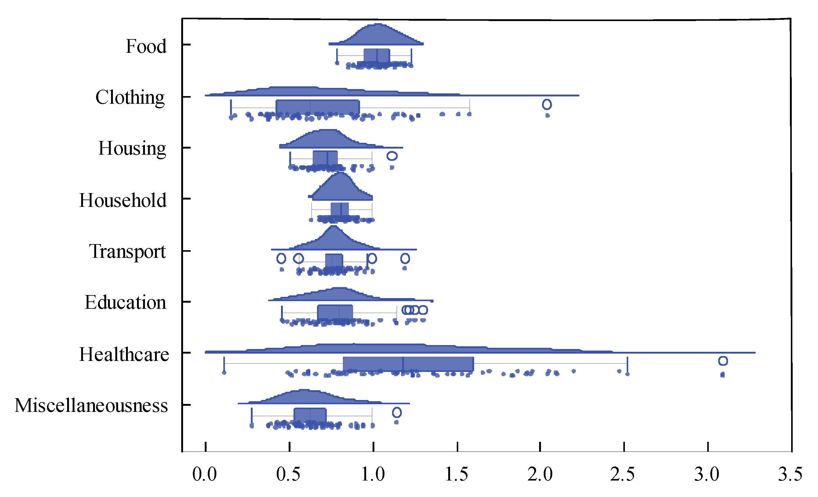
4.2.1. Subnational PPPs of the Eight Main Categories

Firstly, the distribution of the price levels of the eight major categories under urban consumption in China is analyzed, and a raincloud plot of the subnational PPPs in the eight major categories among 76 cities is shown in Figure 2. The raincloud plot can be viewed as a combination figure of a kernel density estimate graph, a box plot, and a scatter chart, which shows the information contained in the data clearly and completely.

As can be seen in Figure 2, there are also significant differences between cities in different categories, with food, tobacco and alcohol; housing; household equipment, furnishings, and services; and transport and communications showing relatively small price fluctuations, but clothing and footwear; education, culture, and recreation; and healthcare and medical services show large differences among cities. This may be due to the fact that the specification commodities under the categories of food, tobacco and liquor; housing; household equipment, furnishings and services; and transport and communications are all tradable commodities, with little geographical variation between cities. In contrast, there are more service commodities in the categories of education, culture and recreation; and healthcare and medical services, which are relatively less homogeneous and comparable, and are non-tradable; the specification commodities under the category of clothing and footwear have strong regional characteristics, and there are also large differences in consumption tendencies between cities, so there are large differences in price levels between cities.

Furthermore, by observing the box plot and the blue circles which represent the outliers of the corresponding major categories of PPPs in Figure 2, it can be seen that the distribution of clothing and transport price levels among 76 prefecture-level cities is characterized by a right-skewed distribution, with most cities having higher price levels and only a few having lower prices. In contrast, the distribution of housing and education price levels among the 76 prefecture-level cities is characterized by a left-skewed distribution, with a higher number of cities having lower price levels. In the remaining categories, there is no clear trend toward higher or lower price levels in the 76 cities.

4.2.2. Subnational PPPs in China

Table 1 gives the results of the subnational PPPs for 76 prefecture-level cities in China. The city with the lowest subnational PPP is Weinan, with a subnational PPP value of 0.615; the city with the highest subnational PPP is Guangzhou, with a subnational PPP value of 1.050. The ratio of the maximum to the minimum subnational PPP is 1.707.

In order to visualize the distribution of subnational PPPs in China, the paper divides 76 cities in China into four major regions and classifies them into four levels: highest, high, low, and lowest, according to the measured subnational PPPs, and the map of the subnational PPPs in 76 cities is shown in Figure 3. Most of the cities with the highest subnational PPPs belong to the eastern region, but there are also a few cities in the central and western regions with high subnational PPPs, such as Liuzhou, Changsha, and Yinchuan; cities with high subnational PPPs are located in the eastern, central, western and northeast regions of China, with more cities in the eastern region. There is a further decline in the proportion of cities in the eastern region at low ranking levels; cities at the lowest ranking levels are more predominant in the central and western regions, with only a few eastern regions with lower subnational PPPs, such as Xingtai and Heze.

It can be seen in Figure 3 that the distribution of subnational PPPs in China is to some extent in line with the trend of decreasing regional economic development levels from east to west, with higher price levels in the east and to a lesser extent in the west, and lower price levels in the central, western and northeast regions. The reason for this trend may be related to the Penn effect, which means that the price level of a country (or region) is positively correlated with the per capita income of that country (or region) [35,36,37]. The more developed economies in the eastern region have higher productivity in the traded goods sector than in the central and western regions, which in turn raises the relative prices of non-traded goods in this region, resulting in relatively higher price levels in the east.

4.3. Analysis of the Real Income Disparity in Prefecture-Level Cities in China

Disposable income refers to the sum of final consumption expenditure and savings available to residents, known as the income available to residents for discretionary use. The per capita disposable income of urban residents has become an important indicator of the changes in the living standards of urban residents in a country (or region). Due to the differences in price levels in prefecture-level cities in China, the directly obtained per capita disposable income of urban residents is a nominal income indicator, which cannot portray the differences in actual income levels between cities, and the actual income levels of regions are underestimated or overestimated. The subnational PPPs measured above are used to deflate the per capita disposable income of urban residents, eliminate the influence of inter-regional price factors, and comparatively analyze the disparity in real income levels in prefecture-level cities in China.

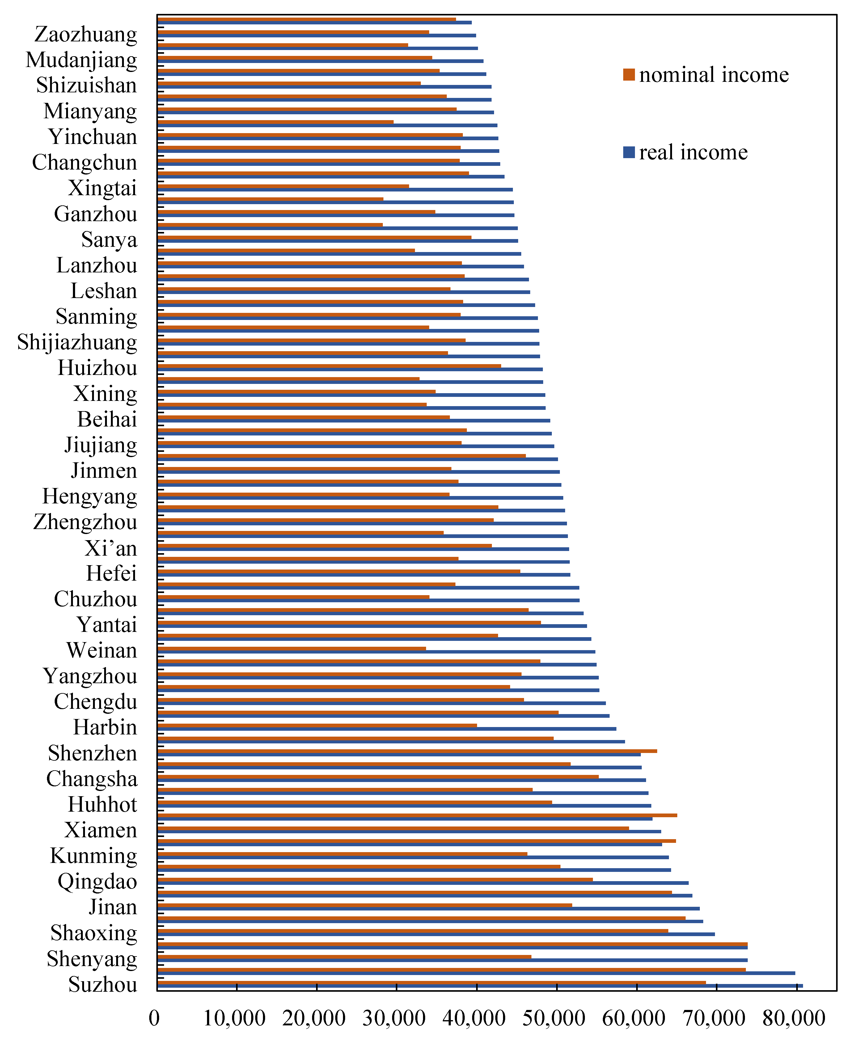
4.3.1. Disparity between Nominal and Real Incomes

In this paper, the subnational PPPs measured by the Rao system under the stochastic approach are used to deflate the per capita disposable income of urban residents in 76 cities in China, defined as per capita real disposable income of urban residents = per capita disposable income of urban residents/subnational PPPs. A comparison of urban disposable income per capita and real income adjusted for subnational PPPs is shown in Figure 4, as follows:

Nominal income is the per capita disposable income of urban residents, sourced from the municipal Statistical Yearbook; real income is the per capita disposable income of urban residents deflated by the subnational PPPs measured by the Rao system under the stochastic approach.

Firstly, using Beijing as the benchmark region, only a few cities experienced a decline in real income levels, such as Guangzhou, Shenzhen, and Ningbo. The rest of the cities showed significant increases in real income levels, with Shenyang and Weinan showing the largest increases in real income at RMB 27,066 and RMB 21,119, respectively, while Liuzhou, Hangzhou, Nanjing, and Tianjin showed relatively small differences between real and nominal income, all below RMB 4000.

Secondly, the degree of real income disparity in prefecture-level cities has narrowed compared to nominal income. The coefficient of variation and the ratio of maximum to minimum values were further used to quantify the extent of regional disparity in the per capita income of urban residents. The coefficients of variation of nominal and real incomes are 0.27 and 0.21, respectively, and the ratios of maximum and minimum values are 2.62 and 2.02, respectively. Both indicators objectively reflect that the gap between the per capita real incomes of urban residents has narrowed to a certain extent compared with nominal incomes, i.e., the gap between the real consumption power of residents in low-income areas and high-income areas is not as large as indicated by nominal incomes.

Thirdly, compared to nominal income, the real income in most cities changed significantly in the national ranking. Among them, the central and western regions showed a significant increase in the real income level compared to the pre-adjustment level, due to the lower price level, while the eastern and coastal regions showed less change. Specifically, the three cities with the highest per capita nominal and real incomes for urban residents were Beijing, Shanghai, and Suzhou in the eastern region, while cities such as Guangzhou, Ningbo, and Shenzhen showed significant declines in their real income rankings, and Weinan, Chuzhou, Shenyang, and Harbin showed significant increases in their real income rankings. The reasons for the above phenomenon are probably related to the impact of the employment structure in a city. More industrialized cities have more inhabitants employed as ordinary workers, while in other cities the professions that dominate may be more profitable. This fact can be equated with regional development, but the nature of the region, such as agricultural, industrialized, and touristic, can also have a big impact and cannot be ignored. For example, in terms of industrial structure, tertiary industries such as tourism and restaurants dominate in cities such as Beijing and Shanghai, so the real income level in these cities is higher than in other manufacturing-dominated cities such as Shenyang and Harbin. Furthermore, considering the nature of the city, the real income level in touristic cities such as Beihai and Kunming is relatively higher than in their neighboring cities.

4.3.2. Geographical Distribution Characteristics of Real Income

Although the gap in per capita real income levels of urban residents between regions in China has narrowed to a certain extent, this is not a reflection of balanced development between regions, and the problem of uneven and insufficient development still exists. In this paper, Getis–Ord Gi* values are calculated separately for nominal and real income, and the study area is divided into hot spot areas, not significant areas, and cold spot areas based on the value of Getis–Ord Gi*. The hot spot areas indicate high-income agglomerations, the cold spot areas are low-income agglomerations, and the insignificant areas indicate insignificant spatial autocorrelation. The spatial agglomeration pattern of nominal income and real income are shown in Figure 5.

As seen visually in Figure 5, the distribution of regional incomes, both in nominal and real terms, generally follows a decreasing trend from east to west, reflecting the uneven and insufficient development of China’s regions. Most cities in the eastern region have higher real incomes, while most cities in the central and western regions have lower incomes, and a few cities in the central and western regions have higher incomes due to their industrial structure, urban characteristics, and geographical advantages.

Furthermore, the hotspot analysis of nominal and real income shows that there is a significant change in the spatial agglomeration pattern of nominal and real income. In terms of nominal income, the high-income agglomeration areas are mainly located in the southeast coastal region. While the spatial agglomeration pattern of real income shows that the range of real income hot spot areas has increased, the high-income agglomeration areas have moved northwards, the level of real income in Shenyang has increased to become a new hot spot area, and the southeast coastal region remains a high-income hot spot area. The cold spot areas for nominal income are located in the central and western regions, such as Weinan, Shizuishan, Hanzhong, and Wuzhong, while the cold spot areas for real income have moved toward the southwest of the country. The cold spot areas for nominal income are no longer cold spots due to lower price levels. Zunyi and its surrounding cities have become the new cold spot area for real incomes due to low nominal incomes and relatively high price levels. In conclusion, real income, excluding the effect of prices, shows a new characteristic, with the real high-income agglomeration moving north and the low-income agglomeration moving southwest, and the real income disparity is not as large as that measured by the nominal income indicator. In terms of real income, the most underdeveloped region is the southwestern part of China.

5. Conclusions, Limitations, and Future Research

5.1. Conclusion and Discussion

This paper introduces a stochastic approach and builds a generalized framework for the multilateral comparative index system under the stochastic approach. The method not only derives an explanation of the internal structure of the traditional index form and measures the subnational PPPs, but also proposes a statistical indicator of heteroskedastic robust standard errors that reflect the quality of the underlying data and the degree of reliability of the results. This indicator not only contains intrinsic economic significance in itself, but also serves as an objective basis for the selection of the subnational PPP measurement method in the preliminary stage and its improvement in the later stage, in order to test the applicability of the subnational PPP measurement method and the underlying data used.

The main findings are as follows. Firstly, the results of the heteroskedastic robust standard error calculations show that the Rao system under the stochastic approach is more reliable, more robust, and more widely applicable than the GK system under the stochastic approach. Compared with the traditional method of measuring PPPs, the Rao system under the stochastic approach and the GK system under the stochastic approach can use price data information as much as possible to avoid information loss. Meanwhile, they can quantify the reliability of the results in order to provide an objective basis for pre-selection and post-improvement of the methodology used. Thus, the improved measurement method in this paper can promote the development of the spatial index theory, and theoretical relevance cannot be ignored.

Secondly, there are objective differences in price levels between cities in China, and the distribution characteristics of subnational PPPs in China are to some extent in line with the trend of decreasing regional economic development levels from east to west, with higher price levels in the eastern regions and a few western regions, and lower price levels in the central, western, and northeastern regions. This suggests that when carrying out analyses of coordinated economic development between regions, income disparities and other livelihood issues, formulating regional economic development strategies, financial transfer allocations and public service project allocation programs, and making regional wage level adjustments, the impact of inter-regional price level differences should be fully taken into account, so that the analysis of problems and policy formulation between regions can be better matched and addressed.

Thirdly, the results of the subnational PPP measurement can accurately measure the difference in real income across cities in China. Compared with nominal income, the real income increased significantly, and the real income disparity between regions narrowed, with the ratio of the highest to the lowest real income in China decreasing from 2.62 to 2.02. By excluding the effect of inter-regional price differences, the real income level of each city and the real income disparity between cities are accurately quantified. A full understanding of how large the income disparity is in China is conducive to the adoption of regionally differentiated measures to promote the realization of common prosperity, which has significant practical relevance.

Finally, real income, excluding the effect of prices, shows a new characteristic of moving toward the north for the high-income agglomeration areas and toward the southwest for the low-income agglomeration areas. At the same time, it is clear from the characteristics of the distribution of the four major regions of real income that both the central and western regions and the eastern regions have greater internal variability, i.e., not all regions in the central and western regions are poor, and not all regions in the eastern regions are developed. It is recommended that, on the basis of in-depth research, problem areas should be scientifically classified, and regional support policies and efforts should be adjusted accordingly. For problematic areas, the government should focus its public investment on people’s livelihoods, so that less developed areas can be given “charcoal in the snow”.

5.2. Limitations

Due to the limitation of the research data, the timeliness of this study needs to be improved. There is currently a lack of accurate and comprehensive price data, which poses many limitations to accurately measuring and comparing real income differences between different regions. Furthermore, this study has not considered the impact of quality factors on the prices of goods and services between regions, and thus the measured price differences between regions are subject to some error.

5.3. Future Research

In terms of research data, it is recommended that the relevant statistical departments, based on the integration of existing price monitoring and collection systems, adopt a combination of regular shop price collection, web data crawling, and text data scanning to update their price information databases, and further improve data quality by using cutting-edge methods such as machine learning to classify the homogeneity of specification items. Real-time, accurate price information is regularly released to the community and used to improve the accuracy and timeliness of regional economic analysis.

Furthermore, in the future, price-related influencing factors such as the quality of goods or services should be fully taken into account, while improving the method of measuring PPPs so that the accuracy of measuring price levels between regions in China is more accurate and reflects the actual situation more accurately.

References

1. Peilin, L.; Tao, Q.; Xianhai, H.; Xuebing, D. The connotation, realization path and measurement method of common prosperity for all. J. Manag. World 2021, 37, 117–129. [Google Scholar]
2. Thomas, C.P.; Marquez, J.; Fahle, S. Measures of international relative prices for china and the USA. Pac. Econ. Rev 2009, 14, 376–397. [Google Scholar] [CrossRef]
3. Ravallion, M. Price levels and economic growth: Making sense of revisions to data on real incomes. Rev. Income Wealth 2013, 59, 593–613. [Google Scholar] [CrossRef]
4. Ray, R.; Singh, P. Regionally disaggregated estimates of global income inequality with evidence on sensitivity to purchasing power parity. J. Asia. Pac. Econ. 2021, 26, 252–270. [Google Scholar] [CrossRef]
5. Osberg, L.; Xu, K. How should we measure poverty in a changing world? Methodological issues and Chinese case study. Rev. Dev. Econ. 2008, 12, 419–441. [Google Scholar] [CrossRef]
6. Deaton, A. Letter from America—It’s a big country, and how to measure it. R. Econ. Soc. 2014, 167, 3–4. [Google Scholar]
7. WorldBank. Purchasing Power Parities and the Size of World Economies: Results from the 2017 International Comparison Program; World Bank: Washington, DC, USA, 2020. [Google Scholar]
8. Asian Development Bank. 2017 International Comparison Program for Asia and the Pacific: Purchasing Power Parities and Real Expenditures—A Summary Report; Asian Development Bank: Mandaluyong, Philippines, 2020. [Google Scholar]
9. Biggeri, L.; Laureti, T.; Polidoro, F. Computing sub-national PPPs with CPI data: An empirical analysis on Italian data using country product dummy models. Soc. Indic. Res. 2017, 131, 93–121. [Google Scholar] [CrossRef]
10. Chamon, M.; de Carvalho, I. Consumption based estimates of urban Chinese growth. China Econ. Rev. 2014, 29, 126–137. [Google Scholar] [CrossRef]
11. Larsen, E.R. Does the CPI mirror the cost of living? Engel’s law suggests not in Norway. Scand. J. Econ. 2007, 109, 177–195. [Google Scholar] [CrossRef]
12. Costa, D.L. Estimating real income in the united states from 1888 to 1994: Correcting CPI bias using Engel curves. J. Polit. Econ. 2001, 109, 1288–1310. [Google Scholar] [CrossRef] [Green Version]
13. Gluzmann, P.; Sturzenegger, F. An estimation of CPI biases in Argentina 1985–2005 and its implications on real income growth and income distribution. Latin. Am. Econ. Rev. 2018, 27, 1–50. [Google Scholar] [CrossRef] [Green Version]
14. Emery, J.C.H.; Guo, X.L. Using an Engel curve approach to infer cost of living experienced by Canadian households. Can. Public Policy Anal. Polit. 2020, 46, 397–413. [Google Scholar] [CrossRef]
15. Chen, M.; Wang, Y.; Rao, D.S.P. Measuring the spatial price differences in china with regional price parity methods. World Econ. 2020, 43, 1103–1146. [Google Scholar] [CrossRef]
16. Aten, B.H. Interarea price levels: An experimental methodology. Mon. Labor Rev. 2006, 129, 47–61. [Google Scholar]
17. Kokoski, M.F. New research on interarea consumer price differences. Mon. Labor Rev. 1991, 114, 31–34. [Google Scholar]
18. Montero, J.M.; Laureti, T.; Minguez, R.; Fernandez-Aviles, G. A stochastic model with penalized coefficients for spatial price comparisons: An application to regional price indexes in Italy. Rev. Income Wealth 2020, 66, 512–533. [Google Scholar] [CrossRef]
19. Majumder, A.; Ray, R.; Sinha, K. Estimating purchasing power parities from household expenditure data using complete demand systems with application to living standards comparison: India and Vietnam. Rev. Income Wealth 2015, 61, 302–328. [Google Scholar] [CrossRef]
20. Aten, B.H. Regional price parities and real regional income for the united states. Soc. Indic. Res. 2017, 131, 123–143. [Google Scholar] [CrossRef]
21. Hearne, D. Regional prices and real incomes in the UK. Reg. Stud. 2021, 55, 951–961. [Google Scholar] [CrossRef]
22. Benedetti, I.; Biggeri, L.; Laureti, T. Sub-national spatial price indexes for housing: Methodological issues and computation for Italy. J. Off. Stat. 2022, 38, 57–82. [Google Scholar] [CrossRef]
23. Jiang, X.J.; Li, H. Smaller real regional income gap than nominal income gap: A price-adjusted study. China World Econ. 2006, 14, 38–53. [Google Scholar] [CrossRef]
24. Biggeri, L.; Ferrari, G.; Zhao, Y. Estimating cross province and municipal city price level differences in china: Some experiments and results. Soc. Indic. Res. 2017, 131, 169–187. [Google Scholar] [CrossRef]
25. Chen, M.G. Sub-national ppps based on house and real income disparity across china: A distinctive spatial deflator. J. Real Estate Financ. Econ. 2021, 62, 187–219. [Google Scholar] [CrossRef]
26. Summers, R. International price comparisons based upon incomplete data*. Rev. Income Wealth 1973, 19, 1–16. [Google Scholar] [CrossRef]
27. Selvanathan, E.; Rao, D.S. Index Numbers: A Stochastic Approach; The University of Michigan Press: Ann Arbor, MI, USA, 1994. [Google Scholar]
28. Diewert, E. New methodological developments for the international comparison program. Rev. Income Wealth 2010, 56, S11–S31. [Google Scholar] [CrossRef]
29. Rao, D.S.P.; Hajargasht, G. Stochastic approach to computation of purchasing power parities in the international comparison program (ICP). J. Econom. 2016, 191, 414–425. [Google Scholar] [CrossRef] [Green Version]
30. Hajargasht, G.; Rao, D.S.P. Stochastic approach to index numbers for multilateral price comparisons and their standard errors. Rev. Income Wealth 2010, 56, S32–S58. [Google Scholar] [CrossRef] [Green Version]
31. Geary, R.C. A note on the comparison of exchange-rates and purchasing power between countries. J. R. Stat. Soc. Ser. a-Gen. 1958, 121, 97–99. [Google Scholar] [CrossRef]
32. Fenoaltea, S. Of economics and statistics: The “gerschenkron effect”. PSL Q. Rev. 2019, 72, 195–205. [Google Scholar]
33. Rao, D.S.P. Chapter 6—A system of log-change index numbers for multilateral comparisons. In Contributions to Economic Analysis; Rao, D.S.P., Ed.; Elsevier: Amsterdam, The Netherlands, 1990; Volume 194, pp. 127–139. [Google Scholar]
34. Research Group on “The Index Method and Application for Regional of Price Difference”. Research on the differentials of regional price level in China. Stat. Res. 2014, 31, 22–30. [Google Scholar]
35. Samuelson, P.A. Facets of balassa-samuelson thirty years later. Rev. Int. Econ. 1994, 2, 201–226. [Google Scholar] [CrossRef]
36. Hassan, F. The price of development: The penn-balassa-samuelson effect revisited. J. Int. Econ. 2016, 102, 291–309. [Google Scholar] [CrossRef]
37. Ishaq, M.; Ghouse, G.; Bhatti, M.I. Another prospective on real exchange rate and the traded goods prices: Revisiting Balassa–Samuelson hypothesis. Sustainability 2022, 14, 7529. [Google Scholar] [CrossRef]
Figure 1. The generalized framework of the multilateral index system under the stochastic approach.
Sustainability 14 09895 g001
Figure 2. The raincloud plot of the subnational PPPs for eight major categories.
Sustainability 14 09895 g002
Figure 3. Map of the subnational PPPs.
Sustainability 14 09895 g003
Figure 4. Bar chart of real versus nominal income.
Sustainability 14 09895 g004
Figure 5. (a) The spatial agglomeration pattern of nominal income; (b) The spatial agglomeration pattern of real income.
Sustainability 14 09895 g005