Assessment of Efficiency of Heat Transportation in Indirect Propane Refrigeration System Equipped with Carbon Dioxide Circulation Loop

Abstract

Recent research on indirect cooling systems using natural refrigerants has become increasingly common. One such solution is the gravity-induced circulation loop. The paper provides model considerations of the configuration of an indirect propane refrigeration system equipped with a circulation loop using carbon dioxide as a heat transfer fluid. Close attention has been paid to the analytical modelling of the carbon dioxide circulation loop operation. The model was formulated to determine the optimum height of the liquid downcomer based on the determination of flow resistance and heat transfer rate in evaporation and condensation processes. A validation of the proposed analytical model against the available literature on two-phase flow structure predictions and thermal performance predictions was performed. The effect of the change in the refrigeration capacity of the system on the coefficient of performance COP of the entire indirect system was analysed for the first time. The analysis was performed for three different carbon dioxide evaporation temperatures for the system’s refrigeration capacity, ranging from 0.5 to 10 kW. It has been proven that the system efficiency increases by up to 23% with an increase in the refrigeration capacity of the system. An increase in evaporation temperature in the circulation loop from −20 °C to 0 °C improves the COP of the entire indirect refrigeration system by approximately 50%. The above findings indicate that indirect cooling systems using naturally circulated CO₂ as a heat transfer fluid should be designed for operation at maximum refrigeration capacity.

1. Introduction

Refrigeration and air-conditioning systems and heat pumps are currently facing many challenges. The European Union introduced increased restrictions on the use of synthetic refrigerants due to their impact on ozone depletion processes and global warming effects. From January 2022, it is not possible to fill refrigeration equipment with refrigerants for which the indicated Global Warming Potential (GWP) is greater than or equal to 150, according to the latest amendment to the Montreal Protocol in Kigali [1]. The Kigali Amendment protects the climate and globally reduces the production and consumption of HFC gases. It introduces a timetable for phasing out the consumption and production of gases with strong greenhouse effects, hydrofluorocarbons, to the Montreal Protocol [2]. It is estimated that implementing the Kigali Amendment will reduce HFC gas emissions by 85% by reducing their production and consumption in all 197 countries—Parties to the Protocol. The above measures practically disqualify a significant portion of the working fluids that have been known for several decades and most of the new substances proposed as ecological substitutes. For the latter, achieving a low global warming impact has often led to a deterioration in their other thermodynamic properties [3]. Therefore, in recent years, there has been a significant increase in the use of natural fluids, mainly carbon dioxide (R744), ammonia (R717), and hydrocarbons, among which the most commonly used are propane (R290) and isobutane (R600a). These substances have a GWP and Ozone Depletion Potential (ODP) close to or equal to zero and have appropriate thermo-physical and chemical parameters that give them advantages over numerous synthetic fluids. However, it is important to note that their other properties sometimes prevent or limit their use. These include their flammability, explosiveness, and toxicity. Then, the application of commercial or industrial refrigeration systems involving their use requires minimising the charge of a given working fluid in the system, for example, using solutions with an indirect system or dividing a given system into several or even smaller systems.

The application of circulation loop with a non-flammable and non-toxic substance as a heat transfer fluid may be thought of as a solution that makes it possible to effectively apply some natural working fluids that are flammable and/or explosive. The Forced Circulation Loop (FCL) systems that use liquid pumping devices can be distinguished. Such solutions are common, e.g., in contemporary supermarket refrigeration systems and solar-collectors-based systems [4,5,6]. The second solution is the Natural Circulation Loop (NCL), where the circulation is conducted by gravity due to the pressure differences produced from the temperature difference and the liquid phase column height. Applying pumping devices to force the NCL system operation is not necessary. As a result, these systems achieve more reliable operation and, additionally, the investment and operating costs of the installation can be significantly reduced. In addition, the NCLs provide safe, quiet, and maintenance-free operation and are very promising solutions to various applications, for example, in refrigeration engineering, nuclear energy [7,8], electronic devices cooling [9,10,11], solar heaters [12], geothermal processes [13], cryogenic refrigeration systems [14], or even domestic refrigerators [15,16].

For NCL, working fluids with suitable thermo-physical properties should be applied to enhance the heat transfer process. The selection of the working fluids could be considered an individual task for each system configuration and its thermal capacity. Researchers compared various potential substances and illustrated the differences between them [17,18]. In recent years, carbon dioxide has been gaining popularity as a working fluid in circulation systems, because it is a non-toxic, non-flammable, and environmentally friendly substance with an indicator GWP equal to one and ODP equal to zero. Thippeswamy et al. [19] conducted an experimental study and confirmed that CO₂ achieves a heat transfer coefficient that is up to nine times higher than water and brine solutions as working fluids. It should be noted that carbon dioxide has a low critical temperature (−31 °C) and critical pressure at 7.37 MPa, which gives it an advantage and uniqueness because it performs well in supercritical conditions. Zhao et al. [20] proposed empirical correlations for natural circulation mass flux for supercritical CO₂ power cycles. The research demonstrated that the pseudo-critical region is the place where the heat transfer process deteriorates. Their results proved that buoyancy forces in a simple circulation loop play a significant role in the heat transfer process. Deng et al. [21] conducted a numerical and experimental study of the application of supercritical CO₂ flows. They observed flows under varying output and input conditions and demonstrated that a supercritical loop could offer very fast stabilisation conditions. The system also responded much faster to condenser adjustments compared to the evaporator. In another study [22], using Nusselt number assessment, researchers have proposed working under supercritical conditions but at the lowest possible pressure to achieve more stable operation conditions of the system. Under higher pressures, they observed bidirectional oscillations and under lower pressure conditions, the loop operation led only to unidirectional pulsations. Thimmaiah et al. [23,24] performed a comparative analysis between two different circulation systems. They proposed an NCL with an isothermal heater and cold heat exchanger and a second NCL with a hot and cold heat exchanger. This study demonstrated the system stability conditions with varying temperature and pressure inside the analysed loop. In addition, the results showed that the supercritical NCL system with an isothermal heater is more stable and has fewer fluctuations in flow rate than the subcritical system.

An especially prominent issue for the NCL design is the appropriate height of the liquid downcomer, because this provides the driving force in the analysed loop. This height is determined by the flow resistance, working pressure, and the amount of liquid phase in a two-phase flow. Bai et al. [25] showed that too large a height results in a larger thermal resistance between the evaporator and condenser. Zhang et al. [26] proposed an ‘’ideal cycle” NCL for refrigeration and air-conditioning applications with a 100% filling ratio. In their simulation, the optimum height of the loop for which the lowest flow resistance occurs was only 1.2 m. In another study, Zhang et al. [27] conducted simulation with a large loop height of up to 10 m in NCL for a refrigeration system. They showed that the large loop height can both enhance or weaken NCL performance because a larger height reinforces circulation but also provides higher thermal resistance. Tong et al. [28] studied three typical operating states in two-phase NCL with carbon dioxide—prestart operation, oscillatory operation, and stable operation state with 100% filling ratio. They examined the loop pipes for 6, 9, and 12 mm diameters and demonstrated that, in addition to appropriate loop height, it is necessary to select adequate diameters of horizontal and vertical pipes depending on the heat load. Tong and Zang [10] conducted research on the diameter of horizontal and vertical pipes for CO₂ thermosyphons used in the data centre. They performed a visual experiment and established a calculation model. The results showed that when the diameter is designed to be too small, the system will be operated under overload conditions; however, when the diameter is too big, the system will be in an oscillatory or inactive state. Therefore, the diameters of the loop pipes should be adjusted to actual heat load. Pegallapati et al. [29] presented a dynamic NCL model using CO₂, which was developed by the balance equations for mass, momentum, and energy. They observed that the wall thermal capacity may also be thought of as a crucial factor in the dynamic operation of NCL because it introduces damping to the system which removes the oscillations and increases the time required to reach steady-state conditions. Tong et al. [30] conducted research on the self-regulating performance of CO₂ in NCL with two evaporators. The results of this study showed that the difference between the heat transfer loads of the parallel evaporators should be as minimal as possible. Otherwise, it is exceedingly difficult to obtain a self-regulation of the loop system because more mass flux is wasted through the low-power evaporator.

As discussed above, much research has been conducted on the diverse types of geometries and numerous applications for NCL with CO₂ as a working fluid in refrigeration systems. An appropriate structure is essential for real applications, so the liquid downcomer, pipes’ diameter, and relevant operation parameters must be carefully selected. However, the aspects of the influence of thermal load of the circulation loop on the efficiency of operation of the entire refrigeration system has never been analysed in the literature, which is the most important motivation of the present paper. This paper presents an approach to the analytical modelling of NCL to determine the optimum height of the liquid downcomer for given boundary conditions and operation parameters.

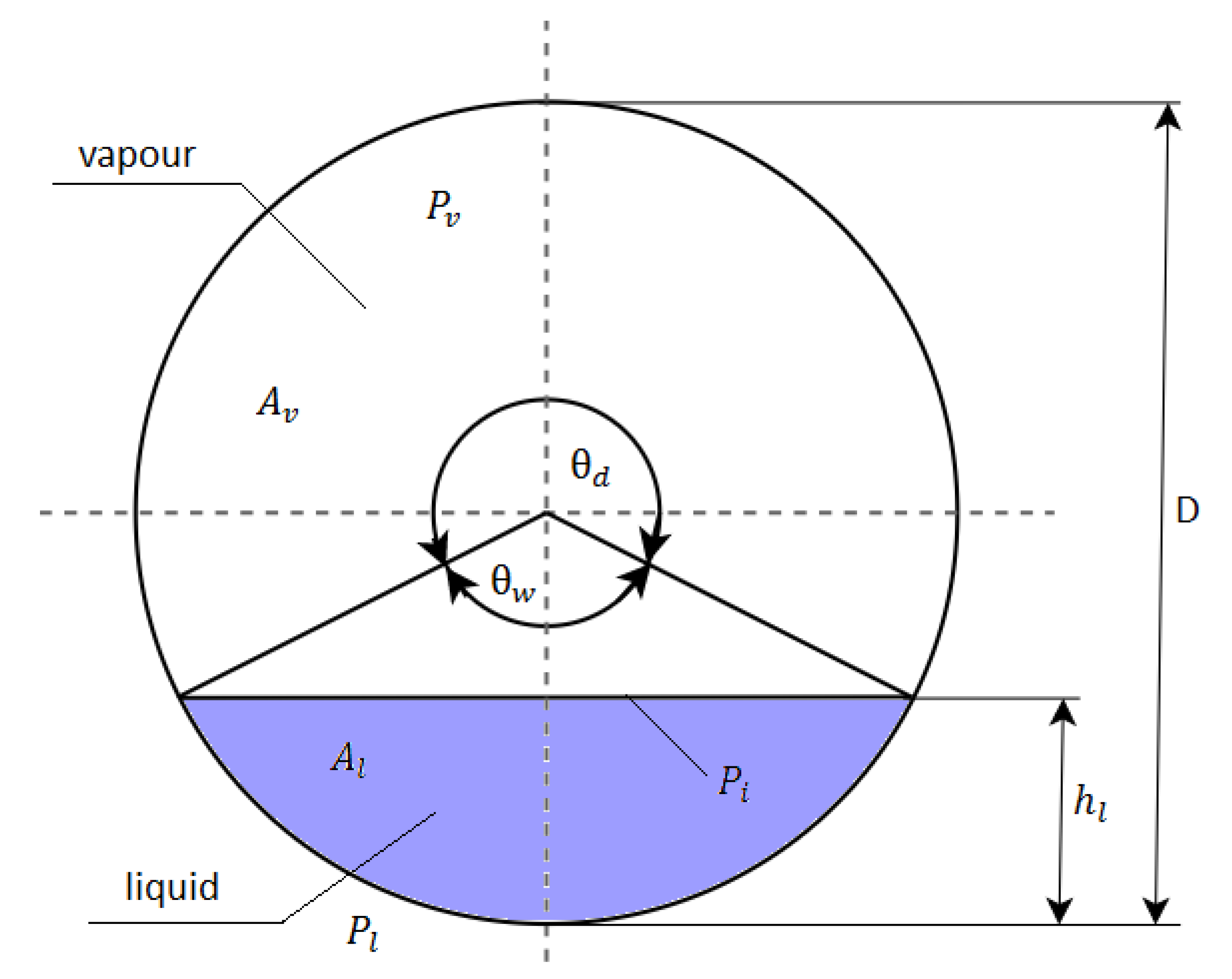
2. Calculation Model

The analysed indirect refrigeration system is presented in Figure 1. The system consists of a propane compressor refrigeration system and carbon dioxide natural circulation loop. It is assumed that the propane chiller has one main refrigeration circuit, consisting of a semi-hermetic reciprocating compressor, plate evaporator and electronic expansion valve, and an auxiliary circuit with an exchanger built into the tank for emergency cooling of CO₂. The unit supplying this circuit is switched on by a signal generated by a pressure alarm pressure switch on the tank, signalling an increase in pressure (usually when the unit does not operate under high external temperature conditions). The second loop is only forced by gravity, where the correct height of the liquid downcomer is essential. An additional issue considered in the system is the possibility of self-regulation of the NCL. Note that the lack of an expansion element reduces investment and operating costs and increases the attractiveness of the system.

To calculate the optimum height of the liquid downcomer, it is necessary to determine the total flow resistance in NCL, which the hydrostatic pressure must overcome, according to the following relation:

$${\rho }_{L}g\mathsf{\Delta }h>\mathsf{\Delta }{p}_c+\mathsf{\Delta }{p}_e+\mathsf{\Delta }{p}_{lt}+\mathsf{\Delta }{p}_{ll} \left[Pa\right]$$

(1)

Flow resistance in the condenser

To calculate the resistance of the two-phase flow in the channels of the plate exchanger, which is a condenser of the CO₂ circuit, empirical correlations are used which include the following formulas proposed by Würfel–Ostrowski [31]:

$${\left(\mathsf{\Delta }{p}_{\lambda }\right)}_k={\left(\mathsf{\Delta }{p}_{\lambda }\right)}_L{\Phi }_{WO}^2.$$

(2)

The pressure loss in single-phase fluid flow is determined as follows:

$${\left(\mathsf{\Delta }{p}_{\lambda }\right)}_L=\lambda \frac{G}{2{\rho }_L}\frac{H_e}{D_h},$$

(3)

where: $\mathrm{G}$—mass flux density of the fluid described by the formula:

$$\mathrm{G}=\mathit{ṁ}\left[\left(1-x\right)+x{\left(\frac{{\rho }_l}{{\rho }_v}\right)}^p\right],$$

(4)

where: p—exponent, dependent on the angle of the channel extrusions of the adjacent heat exchanger plates.

Würfel and Ostrowski [31] have shown that the pressure loss coefficient varies with Reynolds number Re, so that the coefficient can be determined by the formula:

$$\lambda ={\lambda }_{WO}{(\frac{2000}{R{e}_L})}^{0.25},$$

(5)

where: ${\lambda }_{WO}$—coefficient dependent on the angle of the channel extrusions of the adjacent exchanger plates:

$$R{e}_L=\frac{G{D}_h}{{\mu }_L}.$$

(6)

Two-phase flow multiplier ${\Phi }_{WO}$ is a function of the Lockhart–Martinnelli $X_{LM}$ parameter which for turbulent flow is described as follows:

$$X_{LM}={\left(\frac{1-x}{x}\right)}^{0.9}{(\frac{{\rho }_V}{{\rho }_L})}^{0.5}{(\frac{{\mu }_L}{{\mu }_V})}^{0.1},$$

(7)

$${\Phi }_{WO}^2=\frac{F_{WO}}{X_{LM}^2}$$

(8)

where: $F_{WO}$—constant dependent on the angle of the channel extrusions of the adjacent exchanger plates.

Table 1. Loss coefficients for selected loop components acc. to [32].

Regular 90° flanged elbows	0.30
Regular 90° threaded elbows	1.50
Long radius 90° flanged elbows	0.20
Long radius 90° threaded elbows	0.70
Line flow flanged tees	0.20
Line flow threaded tees	0.90
Union threaded	0.08

shows the parameter values based on the design of the exchanger and shows the range of variable condensing parameters that will affect the resistance values.

Flow resistance in the evaporator

The flow resistance in the evaporation process is significantly higher compared to the condensation process. Therefore, the analysis of the pressure loss in this process is necessary, and is determined by the formula:

$$\mathsf{\Delta }{p}_{total}=\mathsf{\Delta }{p}_m+\mathsf{\Delta }{p}_f,$$

(9)

where: $\mathsf{\Delta }{p}_m$—sum of the pressure losses due to momentum difference; $\mathsf{\Delta }{p}_f$—sum of the pressure losses in individual flow structures.

The pressure drop due to momentum difference depends on vapour quality x at the inlet and outlet of the evaporator and the void fraction ε, so it can be determined for a particular fluid flow structure through the evaporator:

$$\mathsf{\Delta }{p}_m=G^2\left[\left[\frac{{\left(1-x_2\right)}^2}{{\rho }_l\left(1-{ϵ}_2\right)}+\frac{x_2^2}{{\rho }_v{\epsilon }^2}\right]-\left[\frac{{\left(1-x_1\right)}^2}{{\rho }_l\left(1-{\epsilon }_1\right)}+\frac{x_1^2}{{\rho }_v{ϵ}_1}\right]\right].$$

(10)

The void fraction inside the analysed channel ε is determined from the relation proposed by Thome and El Hajal [33]:

$$\begin{gathered} \mathsf{\epsilon }=\frac{x}{{\rho }_v}{\left[\left[1+0.12\left(1-x\right)\right]\left(\frac{x}{{\rho }_v}+\frac{1-x}{{\rho }_l}\right) \\ +\frac{1.18\left(1-x\right){\left[g\sigma \left({\rho }_l-{\rho }_v\right)\right]}^{0.25}}{G{\rho }_l{}^{0.5}}\right]}^{-1}. \end{gathered}$$

(11)

Figure 2 shows a schematic of the channel cross-section in two-phase flow with the geometric parameters of the considered two-phase flow.

The provided below geometric parameters are determined from [34]. Dry angle of the pipe circuit ${\mathsf{\theta }}_d$:

$$\begin{gathered} {\mathsf{\theta }}_d=2\pi -2\left[\pi \left(1-\mathsf{\epsilon }\right)+{\left(\frac{3\pi }{2}\right)}^{\frac{1}{3}}\left[1-2\left(1-\mathsf{\epsilon }\right)+{\left(1-\mathsf{\epsilon }\right)}^{\frac{1}{3}}-{\mathsf{\epsilon }}^{\frac{1}{3}}\right] \\ -\frac{1}{200}\left(1-\mathsf{\epsilon }\right)\mathsf{\epsilon }\left[1-2\left(1-\mathsf{\epsilon }\right)\right]\left[1+4{\left(1-\mathsf{\epsilon }\right)}^2+{\mathsf{\epsilon }}^2\right]\right] \end{gathered}$$

(12)

Channel liquid filling height $h_l$:

$$h_l=0.5\left[1-\cos \left(\frac{2\pi -{\mathsf{\theta }}_s}{2}\right) \right].$$

(13)

The ratio of the length of the liquid interface to the filling height in the channel P_i:

$${\mathrm{P}}_{\mathrm{i}}=\sin \left(\frac{2\pi -{\mathsf{\theta }}_s}{2}\right).$$

(14)

Liquid phase cross-section surface area A_l:

$$A_c=\frac{A\left(1-\mathsf{\epsilon }\right)}{D^2},$$

(15)

and vapour phase cross-section surface area $A_v$:

$$A_v=\frac{A\mathsf{\epsilon }}{D^2}.$$

(16)

In a further step, the Froude number Fr and Weber number We for liquid and vapour phase were determined to describe the buoyancy forces on fluid flow phenomena:

$$F{r}_l=\frac{G^2}{{\rho }_l{}^{2}gD},$$

(17)

$$F{r}_v=\frac{G^2}{{\rho }_v\left({\rho }_l-{\rho }_v\right)gD},$$

(18)

$$W{e}_l=\frac{G^{2}D}{{\rho }_l\sigma },$$

(19)

$$W{e}_v=\frac{G^{2}D}{{\rho }_v\sigma }.$$

(20)

Next, the two-phase flow pattern boundaries of the CO₂ two-phase mixture shaped by external, as well as interfacial, forces should be considered. Based on the relation proposed by Cheng et al. [34], the vapour quality is determined by the flow structure changes from intermittent to annular flow regimes because of the large difference in velocity between the two phases, resulting in a large inertial force of the vapour phase:

$$x_{IA}={\left[{1.8}^{1/0.875}{\left(\frac{{\rho }_v}{{\rho }_l}\right)}^{-\frac{1}{1.75}}{\left(\frac{{\mu }_l}{{\mu }_v}\right)}^{-\frac{1}{7}}+1\right]}^{-1}.$$

(21)

The transition boundary between wave flow and intermittent or annular flow is determined from the relationship presented by Kattan et al. [35]:

$$G_{fal}={\left\{\frac{16A_l^{3}gD{\rho }_l{\rho }_v}{x^2{\pi }^2{\left[1-{\left(2h_l-1\right)}^2\right]}^{1/2}}\left[\frac{{\pi }^2}{25h_l^2}\left(\frac{F{r}_l}{W{e}_l}\right)+1\right]\right\}}^{1/2}.$$

(22)

The change in flow structure from a stratified to stratified-wave flow pattern is calculated based on the relationship Kattan et al. [35]:

$$G_{strat}={\left[\frac{{226.3}^2{A}_l{A}_v^2{\rho }_v\left({\rho }_l-{\rho }_v\right){\mu }_{l}g}{x^2\left(1-x\right){\pi }^3}\right]}^{\frac{1}{3}}.$$

(23)

Wojtan et al. [36] presented a criterion for determining the transition of the flow pattern from annular to dry-out, in which the phenomenon of drying the liquid film on the pipeline wall occurs. In the first place, the critical heat flux at which the heat transfer mechanism changes should be determined, and then the limit can be determined:

$$q_{crit}=0.131{\rho }_v{}^{0.5}{h}_l{\left[g\sigma \left({\rho }_l-{\rho }_v\right)\right]}^{0.25}.$$

(24)

The final criterion remained: to determine the boundary of the flow structure from the dry-out to misty flow pattern where the liquid phase of the working mixture disappears:

$$\begin{gathered} G_m={\left\{\frac{1}{0.502}\left[ln\left(\frac{0.61}{x}\right) \\ +0.57\right]{\left(\frac{D}{{\rho }_l\sigma }\right)}^{-0.16}{\left[\frac{1}{gD{\rho }_v\left({\rho }_l-{\rho }_v\right)}\right]}^{0.15}{\left(\frac{{\rho }_v}{{\rho }_l}\right)}^{0.09}{\left(\frac{q}{q_{crit}}\right)}^{-0.72}\right\}}^{1.613}. \end{gathered}$$

(25)

To determine the two-phase flow pattern map for the upstream and downstream vertical oriented channels, the Reynolds number Re for liquid and vapour and the ratio of vapour to liquid density should be determined:

$$R{e}_l=\frac{GD}{{\mu }_l},$$

(26)

$$R{e}_v=\frac{GD}{{\mu }_v},$$

(27)

$${\rho }_r=\frac{{\rho }_v}{{\rho }_l}.$$

(28)

In addition, the relationships proposed by Schmid [37] to predict the vapour quality of borders of particular flow patterns are used. The boundary of changes in flow pattern from bubble to plug flow pattern during upward flow is as follows:

$$x_{b-s,up}=17.614F{r}_v^{0.423}R{e}_l^{-0.772}W{e}_v^{-0.176}.$$

(29)

Boundary of change in flow pattern from bubble to plug structure during downward flow:

$$x_{b-s,down}={1.310}^{-7}F{r}_v^{1.933}R{e}_l^{0.102}W{e}_v^{0.227}.$$

(30)

Boundary of change in flow pattern from plug type to churn flow during upward flow:

$$x_{s-p,up}=2.225F{r}_l^{0.973}R{e}_l^{-1.266}R{e}_v^{1.463}W{e}_v^{-0.721}{\rho }_r{}^{0.809}.$$

(31)

Boundary of change in flow pattern from plug type churn during downward flow:

$$x_{s-p,down}=2.604F{r}_l^{1.068}R{e}_l^{-2.299}R{e}_v^{1.435}W{e}_v^{0.588}{\rho }_r{}^{0.923}.$$

(32)

Boundary of change in flow pattern from churn flow to annular during upward flow:

$$x_{p-a,up}=2.445F{r}_l^{-0.342}R{e}_l^{-0.836}R{e}_v^{0.525}W{e}_v^{0.244}{\rho }_r{}^{0.509}.$$

(33)

Boundary of change in flow pattern from plug flow to annular during downward flow:

$$x_{p-a,down}=4.108F{r}_l^{-2.902}R{e}_l^{-4.077}R{e}_v^{2.296}W{e}_v^{2.463}{\rho }_r{}^{2.745}.$$

(34)

To determine the heat transfer surface of the evaporator, the average heat transfer coefficient k is determined for each of the flow structures that occurs in the exchanger by determining the liquid and vapour coefficients, and the boundary of change for the flow structure. The liquid phase heat transfer coefficient depends on the Reynolds number Re, Prandtl number Pr, thermal conductivity λ and the inner diameter of the pipeline D [38]:

$$Pr=\frac{C_p\mu }{\lambda },$$

(35)

$$k_l=0.023R{e}^{0.8}P{r}^{0.4}\frac{\lambda }{D} .$$

(36)

The heat transfer coefficient is determined for each boundary of the flow structures. In addition, it is necessary to determine the reduced pressure, which is the ratio of the evaporation pressure to the critical pressure:

$$p_{red}=\frac{p_e}{p_{crit}},$$

(37)

$$k_x=k_l\left[{\left(1-x\right)}^{0.8}+\frac{3.8x^{0.76}{\left(1-x\right)}^{0.04}}{p_{red}^{0.38}}\right].$$

(38)

The average heat transfer coefficient for each flow pattern is determined by averaging the three heat transfer coefficient results as a function of vapour quality:

$$k_{av}=\frac{k_{x1}+k_{x2}+k_{x3}}{3}.$$

(39)

Then, the internal temperature of the evaporator should be calculated as follows:

$$T_{in}=\frac{\frac{{\lambda }_{pipe}}{\delta }{T}_{out}+k_{av}{T}_{vap}}{\frac{{\lambda }_{pipe}}{\delta }+k_{av}}.$$

(40)

Finally, the heat transfer surface areas H and evaporator coil lengths L should be determined for each flow pattern, as follows:

$$H=\frac{Q_e}{k_{av}\left(T_{in}-T_e\right)},$$

(41)

$$L=\frac{H}{\pi D}.$$

(42)

In a further step, the frictional flow resistances for each of the two-phase flow patterns should be determined. The annular flow begins with the use of Moreno Qubein’s and Thom’s correlations [39], which considers the Fanning friction coefficient for the selected flow pattern:

$$f_{an,p}=3.128R{e}_v{}^{-0.454}W{e}_l{}^{-0.0308}.$$

(43)

The averaged sum of frictional pressure losses in two-phase annular flow is determined at the beginning and end of the annular structure flow regime:

$$\mathsf{\Delta }{p}_{pp}=4f_{an}\frac{L_p}{D}\frac{{\rho }_v{u}_v{}^2}{2}.$$

(44)

To calculate the pressure loss in the intermittent flow pattern, the same relationships may be applied as for the annular flow. However, the calculation of the Fanning friction coefficient for the given flow pattern, calculated according to the following relationship [40], is applied:

$$f_{an,i}=0.079R{e}_l^{-0.25}.$$

(45)

The Fanning friction factor for the misty flow is then determined according to the correlation [39], and the pressure losses were determined, as in the previous flow structures:

$$f_{an,m}=\frac{91.2}{R{e}_m{}^{0.832}}.$$

(46)

For the dry-out flow pattern, the average heat transfer coefficients k was determined for two vapour-quality limits, i.e., when changing the flow pattern from intermittent to dry-out and when changing the dry-out to misty flow. Using the correlation [32], the average value of the frictional pressure drop was determined:

$$\mathsf{\Delta }{p}_d=\mathsf{\Delta }{p}_{id}-\frac{x_{av}-x_{id}}{x_{dm}-x_{id}}\left(\mathsf{\Delta }{p}_{id}-\mathsf{\Delta }{p}_{dm}\right).$$

(47)

Flow resistance along the pipeline length

It is necessary to calculate the total resistances in the circulation loop to determine and design the appropriate height of the liquid downcomer in the proposed system. The change in the density of the working fluid due to the variation in condensation and evaporation saturation conditions should be treated as important parameters. These variations will also significantly affect the required height of the liquid downcomer. The computational model, therefore, enables the initiation of planned experimental studies and helps to understand the effects of the various parameters on the variation in the required height.

To calculate the flow resistance along the length in a specific section of a liquid or vapour section, the Darcy–Weisbach [32] relation was applied:

$$\mathsf{\Delta }{p}_{lenght}=\lambda \frac{L}{D_i}\frac{\rho w^2}{2}.$$

(48)

The linear resistance factor $\lambda$ is a function of the Re number and the relative roughness e dimension:

$$\lambda =f\left(Re, e\right)$$

(49)

To determine this coefficient, a Moody’s diagram should be applied, which is available in the literature [41]. Using the above diagram, the coefficient of losses in length can be determined for each value of the calculated Reynolds number. However, analytical relationships are available that allow for the coefficient to be determined. In the case of laminar flow, the coefficient is determined using the Hagen–Poiseuille equation [42]:

$${\lambda }_{laminar}=\frac{64}{Re}.$$

(50)

In the case of turbulent flow in hydraulically smooth pipes, the Prandtl–Karman formula is used [42]:

$${\lambda }_{turbulent\left(smooth\right)}={\left(2\log \frac{\sqrt{\lambda } Re}{2.51}\right)}^{-2}.$$

(51)

On the other hand, for a rough pipeline in turbulent flow, the Swamme and Jain relation can be used [42]:

$$\frac{1}{\sqrt{{\lambda }_{turbulent\left(rough\right)}}}=2\log \left(\frac{5.74}{R{e}^{0,9}}+\frac{e}{3.7}\right)$$

(52)

In addition to the flow resistance in the gas riser pipe, the gravitational losses exerted by the gas must be added:

$${\mathsf{\Delta }}_{p,gas}=\mathsf{\rho }gh$$

(53)

Local flow resistance

Local pressure losses are caused by all components in the pipe, such as valves, bends, changes in cross-section, etc. The local pressure losses are described by the following equation:

$$\mathsf{\Delta }{p}_{local}={\xi }_{local}\frac{\rho w^2}{2}.$$

(54)

The loss coefficient ${\xi }_{local}$ depends on the geometry of the element that causes the loss and is usually determined experimentally. Some of the coefficients that were applied for the loop calculations are listed in Table 1.

In the case of valves, the loss coefficient will be much higher; therefore, if the system under test is self-regulating, then the use of additional fittings should be avoided. In addition, it is especially important to design the system to minimise the occurrence of flow changes from vertical to horizontal and vice versa, as well as to minimize the number of pipeline bends.

3. Model Validation

3.1. Validation of Two-Phase Flow Pattern Prediction

Section 2 shows that the prediction of pressure drops and heat transfer is based on the prediction of a two-phase flow pattern. To validate the proposed analytical model, the predictions of a two-phase flow pattern are compared with the available literature providing experimental investigation results.

Gasche [43] conducted an experimental study of CO₂ evaporation for various mass velocities in a microchannel. He observed the diverse types of flows, depending on the vapour quality. The flow patterns that were experimentally obtained by Gasche [43] are presented in Figure 3. Note that two-phase pattern boundaries are predicted with the use of the formulated analytical model. As can be seen from the two-phase flow pattern map, the prediction of flow pattern types agrees with the experimental data of Gasche [43], especially for the annular region.

The second example is an experimental study on the observation of flow structures during boiling in CO₂ flow at a high pressure in small-diameter tubes [44]. Figure 4 provides the identified CO₂ flow pattern in a 2 mm diameter pipe at a pressure of 5 MPa.

Figure 4 provides the observed individual flow structures for the corresponding vapour quality. Points were determined for two mass velocities related to the pipeline cross-section: 300 kg/m²⋅s and 700 kg/m²⋅s. Researchers observed the initial flow as bubbly, which is more often attributed to vertical flows and is not highlighted in the proposed flow pattern map. Plug flow has been reported in the literature; hence, in the map, this is shown as a stratified-wavy flow [34]. Accordingly, it can be seen that three of the four points marked on the proposed map agree very well with experimental observations for both mass velocities. The disputed place is the dry-out region. This provides an introduction to the misty region, which is not always highlighted in studies [43]. Therefore, the validation showed that the loop design method proposed in this paper shows its compatibility with other studies available in the literature.

3.2. Validation for Thermal Performance Prediction

The proposed analytical model makes it possible to predict the optimum loop height between heat exchanger locations that could be validated with NCL experimental data. Tong and Zang [10] conducted an experiment on the change in pipeline diameter on loop operation, with CO₂ as a working fluid. The research proposed a model with a temperature difference between condensation and evaporation of close to zero. The proposed circulation loop, along with the applied operation parameters, is shown in Figure 5 for a pipeline diameter of 10 mm.

Based on the parameters shown in Figure 5, the specific enthalpies at the inlet and outlet of the evaporator were read from the Coolprop software, as follows: $h_{in}=261.15\frac{\mathrm{k}\mathrm{J}}{\mathrm{k}\mathrm{g}}$; $h_{out}=404.45\frac{\mathrm{k}\mathrm{J}}{\mathrm{k}\mathrm{g}}$. These data made it possible to determine the mass flux of the working fluid:

$$G=\frac{Q}{h_o-h_i}\frac{4}{\pi D_i^2}=337.64 \left[\frac{\mathrm{kg}}{{\mathrm{m}}^2·\mathrm{s}}\right]$$

The value measured in the experiment [10] was $G=362 [\frac{\mathrm{kg}}{{\mathrm{m}}^2·\mathrm{s}}]$. The difference in height between the exchangers was 1.23 m. This altitude allows for the hydrostatic pressure at given parameters to reach 9.125 kPa. This means that the total resistance in the circulating loop must be lower than the pressure that must be exerted by the column of liquefied fluid for the system to achieve its stable operation. The resistances in the vapour and liquid pipelines were determined from the analytical model presented in Section 2, and the predicted pressure drop due to flow resistances for the entire loop is 3.56 kPa. Subtracting these two values from each other results in 5.565 kPa. Therefore, this is the maximum total resistance in the evaporator and condenser. The resistance in the exchangers was not calculated due to the unknown structure of the exchangers. However, the obtained results may be assessed to correspond to the order of magnitude of pressure drops in the plate heat exchangers’ application to the evaporator and condenser according to the calculated flow resistance values in heat exchangers of the proposed model, as shown in

Table 2. Assumed CO₂ condenser and evaporator geometries (based on existing plate heat exchangers) acc. to [45].

CO2 Condenser		CO2 Evaporator
Angle of embossing of the channels of adjacent plates ϒ	60°/30°	Angle of embossing of the channels of adjacent plates ϒ	30°/30°
$F_{WO}$	0.10	$F_{WO}$	0.10
p	0.30	p	0.40
${\lambda }_{WO}$	1.0	${\lambda }_{WO}$	0.86
H [m]	0.50	H	0.30
$d_h$[m]	0.002	$d_h$	0.0018
Plate width [m]	0.145	Plate width	0.150
Heat transfer area [m2]	1.015	Heat transfer area	1.80
Predicted flow resistance depends on mass flux in terms of 0.005–0.05 kg/s [kPa]	0.67–1.64	Predicted flow resistance depends on mass flux in terms of 0.005–0.05 kg/s [kPa]	3.59–10.26

.

Yang X. et al. [46] proposed a practical design method for NCL used in refrigeration systems. They determined the recommended diameter and minimum height difference between heat exchangers with a heat transfer rate of up to 10 kW. They presented a loop design method for five different working fluids, including CO_2. In the proposed design method, they presented pipeline diameters for particular heat transfer capacities, which are most optimal from an economic perspective. They also determined the minimum height difference between the heat exchangers.

Table 3. Comparison of model prediction with experimental results of Yang X. et al. [46].

Q	Diameter of Pipe	Experimental Loop Height and Pressure Losses	Calculated Loop Height and Pressure Losses
4000 W	12.7 mm	0.65 m; 7.83 kPa	0.89 m; 10.72 kPa
8000 W	15.9 mm	0.75 m; 9.04 kPa	0.94 m; 11.33 kPa
10,000 W	19.1 mm	0.40 m;4.82 kPa	0.65 m; 7.83 kPa

presents a comparison of the design recommendations on height difference made by the researchers with the results of the calculations proposed in this article. R134a was chosen for comparison, as a detailed analysis of this fluid was conducted by researchers. The temperature of the R134a was taken as 20 °C and the length of circuit pipeline as 10 m. According to Equation (1), each additional 1 kPa of pressure loss in the loop results in a need to increase the liquid downcomer by 0.083 m. For validation purposes, the condenser flow resistance of 0.7–1.0 kPa and evaporator flow resistance of 3.7–6.0 kPa were assumed. The inaccuracies when determining resistance in the exchangers is crucial to all validation.

The available literature experimental results do not cover all the necessary data concerning components of the tested systems, e.g., the exact data of applied heat exchangers and all fitting elements. The proposed modelling approach requires that these data are applied to the accurate prediction of flow resistance in the analysed system. Therefore, the difference between prediction and experimental results is attributed to both the accuracy of model prediction and additional pressure losses in the system that were not accounted for in calculations (mostly internal pressure losses in heat exchangers), as exact data were not provided in the literature sources. The obtained results may be assessed to correspond to the order of magnitude of the pressure drops in the plate heat exchangers when applied to the evaporator and condenser that are considered in Section 4 (see Table 2). For validation purposes, a condenser flow resistance of 0.7–1.0 kPa and evaporator flow resistance of 3.7–6.0 kPa were assumed for the analysis.

4. Results and Discussion

To analyze the operation of the circulation, it is necessary to assume the geometry of the heat exchangers. Table 2 provides information about the condenser and evaporator geometries obtained for the real propane system equipped with a CO₂ circulation loop.

The main design problem is to ensure a stable natural refrigerant flow due to heat transportation in the evaporator and condenser and achieve the lowest possible pressure loss in the NCL. When designing, it is necessary to pay attention to the limitations that may occur at equipment locations. Flow resistance in the pipelines largely depends on the length of the pipelines, their diameter, and the set of bends that may result from the circulation loop application conditions. It is important that this system can work in open conditions and does not require a height that would make this difficult, and sometimes impossible, to apply such systems. With the present considerations, based on the conditions of possible applications in commercial refrigeration systems, the assumed maximum height of the liquid downcomer is 4 m. For the system to work automatically, the hydrostatic pressure of the liquefied refrigerant must be greater than the total flow resistance in the circulation loop. The relationship between the hydrostatic pressure values of a column of liquefied CO₂ as a function of the condensation temperature is presented in Figure 6. The presented results provide information about the maximum allowable total flow resistance of the analysed NCL. The presented results indicate that the effect of CO₂ condensation temperature, which may be thought as a kind of free parameter of the analysed refrigeration system, plays a crucial role in the design of this system.

As can be seen from the above graph, increasing the condensation temperature from −12 to +2 °C reduces the hydrostatic pressure by over 3 kPa which makes 8% difference between the maximum and the minimum pressure difference. This is due to the thermodynamic parameters of CO₂ and, more specifically, its density. It is, therefore, important to consider the condensation parameters at the design stage, as they can significantly affect the system’s stable operation. Due to the gravitational nature of the fluid flow and the lack of influence on the pressure exerted by the liquid column, the flow resistance created in the condenser and on the path between the condenser and the liquefied CO₂ tank is negligibly small, as it does not exceed 300 Pa. A suitably designed condenser, using a small amount of refrigerant, ensures the removal of high-heat flux density with a significantly low flow resistance.

Another particularly important aspect of NCL design is selection of the appropriate length and diameter of the pipeline. Every increase in the length of the pipeline causes additional flow resistance. An optimised design should be based on the selection of an optimum pipeline diameter depending on the possibility of reaching the optimum height of the liquid downcomer, where the length of the pipeline results from the installation configuration that matches the application conditions. Therefore, the objective of the NCL design is to achieve a system capacity that can meet the required refrigeration capacity. Zhang et al. [20] proposed that NCL modelling should be optimised to obtain parameters that are close to the “ideal cycle”, which is described as a cycle without flow resistance along the length at a pipeline. To describe such a cycle, it is necessary to know the heat transfer coefficient of the heat exchangers and their heat transfer surfaces F. Then, it is assumed that, in the evaporator, pool boiling heat transfer occurs without cooling and vapour superheating regions. Then, the Cooper heat transfer correlation [47] can be used to calculate the heat transfer coefficient:

$$h_{evaporator}=55p_r{}^{0.12-0.2lo{g}_{{10}^{\left(\mathsf{\varepsilon }\right)}}}{\left(-lo{g}_{10}{p}_r\right)}^{-0.55}{M}^{-0.5}{q}^{0.67}.$$

(55)

In an ideal cycle, a stratified flow pattern is assumed in the condenser, without regions of liquid subcooling and no vapour superheating. This allows us to describe the Nusselt film condensation model [20] for condensation in tubes:

$$h_{condensator}=1.47R{e}^{-\frac{1}{3}}{\left(\frac{{\rho }_l\left({\rho }_l-{\rho }_v\right)g}{{\mu }_l^2}\right)}^{1/3}{\lambda }_l.$$

(56)

Then, the heat transfer rate Q_idealfor the “ideal cycle” can be determined from equation [20]:

$$Q_{ideal}=\frac{T_{source}-T_{sink}}{\left(\frac{1}{h_c{F}_c}+\frac{1}{h_e{F}_e}\right)+\left(R_e{R}_c\right)}$$

(57)

It is certain that the tested real system will deviate to a greater or lesser extent from “ideal cycle.” Researchers [20] suggested a definition of the degree of approximation of χ of the $Q_{real}$ to the $Q_{ideal}$:

$$\chi =\frac{Q_{real}}{Q_{ideal}}.$$

(58)

To accurately determine $Q_{real}$, it is necessary to perform experimental studies. Then, the determination of χ will involve correlating design assumptions and model calculations with experimental studies.

Staying with the “ideal cycle” assumptions, note that, in this case, the condensation temperature of the refrigerant is the same as the evaporation temperature. In terms of NCL modelling with CO₂, the difference in these temperatures is particularly important due to the properties of carbon dioxide. An increase in the temperature difference $t_e$ and $t_c$ will necessitate an increase in the liquid downcomer, which can enable NCL operations and achieve self-adjustment of refrigerant mass flux. Therefore, a minimum temperature difference must be achieved to ensure system operation. In addition, the diameter of the pipeline is closely related to temperature differences. Figure 7 shows the calculated dependence of the necessary height difference in the liquid downcomer on the difference between evaporation and condensation temperatures for various pipeline diameters.

In the above graph, the larger diameter of the pipeline achieves better results for given height differences in the liquid downcomer. The larger diameter of the pipeline results in a higher mass flux in the working fluid and can be still a more attractive choice for loop design due to its ability to manage higher actual heat loads. Of course, it should be noted that larger pipeline diameters lead to increase in the investment costs of the circuit, especially in the case of special vapour pressure pipes for CO₂.

The most important aspect, however, is the assessment of the effect of refrigeration capacity for circulation loop operation for the NCL system, in which the height difference and selected pipeline diameters were already designed and remained the same. Then, the effect of changing the NCL heat load, as well as the evaporation temperature of CO₂ on the energy efficiency of the entire system, consisted of a propane refrigeration unit and CO₂ circulation loop. The assumed height of the liquid downcomer is 4 m, and the diameter of the pipeline is 18 mm. The variable parameter of the refrigeration capacity of the evaporator ranged from 0.50 kW to 10 kW. In Figure 8, prediction results that show the dependence of the mass flux of the working fluid and the temperature difference between the change in heat exchangers for the designed system, depending on the heat load. As noted, as the heat capacity increases, the mass flux of the circulating working fluid increases and the temperature difference increases by increasing the condensation temperature at a constant evaporation temperature. This means that the condenser is responsible for the generation of the pressure that is necessary for the working fluid circulation in the loop. These parameters are responsible for the flow circulation adjustment under a variable heat load (i.e., refrigeration capacity) in the analysed system. This may be thought of as the key aspect in the application of the analysed system.

Figure 9 shows a diagram of the system considered in this paper. It is composed of an R290 refrigeration unit and circulation loop with CO_2.

In addition, it is necessary to consider the consequences of the NCL operation’s response to the energy efficiency of the entire refrigeration system, which consisted of a propane refrigeration unit and CO₂ circulation loop. The refrigeration unit and circulation loop are coupled in the CO₂ condenser, which, in turn, acts as an evaporator for the propane cycle. In practice, this means that, as the condensation temperature of CO₂ increases, the evaporation temperature of propane in the plate exchanger should also increase. However, increasing the evaporation temperature of propane refrigeration unit will directly increase the coefficient of performance (COP) of this system, as this is the primary means of improving this indicator, as can be seen from the following formula:

$$COP=\frac{Q_o}{P},$$

(59)

where $Q_o$ is refrigeration capacity, and P is the motive electric power of the compressor of the propane refrigeration unit. The motivating power to drive the refrigeration unit can be determined according to the formula:

$$P=\mathit{ṁ}\mathsf{\Delta }h,$$

(60)

where ∆h is the enthalpy difference in the refrigerant (propane) produced by the compressor. Based on the difference between the specific enthalpy of a saturated liquid at the condensation temperature h_in and specific enthalpy of a saturated vapour at the evaporation temperature h_out in propane refrigeration unit, we can calculate the required mass flux that should be compressed by the compressor:

$$\dot{m}=\frac{Q_o}{h_{out}-h_{in}}$$

(61)

Let us assume, for the system under consideration, that the condensation temperature of propane is 40 °C. The evaporation temperature of propane will depend on the operation parameters of the NCL. To determine the evaporation temperature of propane, it is necessary to determine the heat transfer coefficient of the plate heat exchanger between the considered working fluids (propane and carbon dioxide). The assessment of evaporation heat transfer of propane may be conducted by using the following heat transfer correlation [42]:

$$Nu=0.022\sqrt{{\zeta }_0}\beta {\beta }_{t}R{e}^{0.825}P{r}^{0.54},$$

(62)

where the necessary values are defined as follows:

$$Re=\frac{w{D}_h\mathsf{⍴}}{\mu },$$

(63)

$${\zeta }_0=\frac{0.3164}{R{e}^{0.25}},$$

(64)

$${\beta }_t=1+\left(-\frac{0.66D_0}{D_h}\right)ln\frac{4.23\left(0.65+1.07lg\frac{D_h}{D_0}\right)}{0.3164},$$

(65)

$$\beta =4-\frac{1.65D_0}{D_h}.$$

(66)

Boiling side heat transfer coefficients k and overall heat transfer coefficient U may then be calculated using the following formulas:

$$k=\frac{Nu\lambda }{D_h},$$

(67)

$$U=\frac{1}{\frac{1}{k_{\mathrm{C}\mathrm{O}2}}+\frac{\delta }{\lambda }+\frac{1}{k_{R290}}}$$

(68)

Based on the overall heat transfer coefficient, the temperature difference in the plate exchanger can be determined using the refrigeration capacity and heat transfer surface area of the heat exchanger:

$$\dot{Q}=AU\mathsf{\Delta }\mathrm{T}.$$

(69)

For comparison, three different evaporation temperatures of CO₂ were assumed: −20 °C, −10 °C, and 0 °C. The results are shown in

Table 4. Calculation results of propane evaporator/CO₂ condenser and resulting circulation CO₂ loop temperature difference.

$\mathbf{Parameters} \mathbf{of} \mathbf{the} \mathbf{Condensation} \mathbf{C}{\mathbf{O}}_{\mathbf{2}} \mathbf{side} \mathbf{\to }\mathbf{-}\mathbf{20} \mathbf{°}\mathbf{C}$
Re	Pr	${\zeta }_0$	${\beta }_t$	$\beta$	Nu	$k_{\mathrm{C}{\mathrm{O}}_2}$$\mathbf{[}\frac{W}{m^{2}K}]$	$\mathrm{U} \left[\frac{W}{m^{2}K}\right]$	ΔT°C
14,820	2.23	0.029	2.98	3.59	170.5	5754	1543.2	1.67
Parameters of the evaporation R290 side
Re	Pr	${\zeta }_0$	${\beta }_t$	$\beta$	Nu	$k_{\mathrm{R}290} \left[\frac{W}{m^{2}K}\right]$
5710	1.75	0.036	2.99	3.59	76.13	2227
$\mathbf{Parameters} \mathbf{of} \mathbf{the} \mathbf{condensation} \mathbf{C}{\mathbf{O}}_{\mathbf{2}}$ side→−10 °C
Re	Pr	${\zeta }_0$	${\beta }_t$	$\beta$	Nu	$k_{\mathrm{C}{\mathrm{O}}_2}$$\mathbf{[}\frac{W}{m^{2}K}]$	$\mathrm{k} \left[\frac{W}{m^{2}K}\right]$	ΔT °C
16,657	2.2	0.028	2.98	3.59	183.25	5613.9	1658.4	1.56
Parameters of the evaporation R290 side
Re	Pr	${\zeta }_0$	${\beta }_t$	$\beta$	Nu	$k_{\mathrm{R}290} \left[\frac{W}{m^{2}K}\right]$
6190	2.16	0.036	2.98	3.59	90.95	2509.2
$\mathbf{Parameters} \mathbf{of} \mathbf{the} \mathbf{condensation} \mathbf{C}{\mathbf{O}}_{\mathbf{2}}$ side→0 °C
Re	Pr	${\zeta }_0$	${\beta }_t$	$\beta$	Nu	$k_{\mathrm{C}{\mathrm{O}}_2}$$\mathbf{[}\frac{W}{m^{2}K}]$	$\mathrm{k} \left[\frac{W}{m^{2}K}\right]$	ΔT °C
18,662	2.27	0.027	2.98	3.59	201.01	5549.38	1855.29	1.39
Parameters of the evaporation R290 side
Re	Pr	${\zeta }_0$	${\beta }_t$	$\beta$	Nu	$k_{\mathrm{R}290}$$\mathbf{[}\frac{W}{m^{2}K}]$
6684	2.95	0.035	2.98	3.59	113.01	2993.92

.

Based on the calculations, the required temperature differences between CO₂ condensation and CO₂ evaporation of lower than 2 K have been obtained. Based on these temperature differences, the required mass flux in propane in the propane refrigeration unit, the electrical power consumed by the compressor and the results are shown in the

Table 5. Predicted required operation parameters for the propane refrigeration unit.

Evaporation Temperature of CO2 → −20 °C
Heat Load of NCL [kW]	Mass Flux of CO2 [kg/s]	Evaporation Temperature of Propane [°C]	Mass Flux of Propane [kg/s]	Enthalpy Difference ∆h [kJ/kg]	Power of the Compressor P [kW]
500	0.00177	−21.37	0.00650	64.19	0.414
1500	0.00531	−20.77	0.00652	62.86	0.410
2500	0.00885	−20.07	0.00654	62.05	0.406
3500	0.01240	−19.37	0.00655	61.23	0.401
4500	0.01593	−18.67	0.00657	60.42	0.397
5500	0.01947	−17.97	0.00658	59.61	0.392
6500	0.02301	−17.17	0.00660	58.68	0.387
7500	0.02655	−16.37	0.00661	57.75	0.382
8500	0.03009	−15.57	0.00663	56.83	0.377
9500	0.03363	−14.77	0.00665	55.91	0.372
10,000	0.03541	−14.27	0.00666	55.33	0.369
Evaporation temperature of CO2→ −10 °C
Heat load of NCL [kW]	Mass Flux of CO2 [kg/s]	Evaporation temperature of propane [°C]	Mass flux of propane [kg/s]	Enthalpy difference ∆h [kJ/kg]	Power of the compressor P [kW]
500	0.00193	−11.24	0.00672	51.96	0.349
1500	0.00580	−10.64	0.00673	51.29	0.345
2500	0.00967	−9.94	0.00675	50.49	0.341
3500	0.01353	−9.24	0.00676	49.70	0.336
4500	0.01740	−8.54	0.00678	48.90	0.332
5500	0.02127	−7.84	0.00680	48.11	0.327
6500	0.02514	−7.04	0.00681	47.32	0.322
7500	0.02900	−6.24	0.00683	46.42	0.317
8500	0.03287	−5.44	0.00685	45.52	0.312
9500	0.03674	−4.54	0.00687	44.51	0.306
10,000	0.03867	−4.04	0.00689	43.95	0.303
Evaporation temperature of CO2→0°C
Heat load of NCL [kW]	Mass Flux of CO2 [kg/s]	Evaporation temperature of propane [°C]	Mass flux of propane [kg/s]	Enthalpy difference ∆h [kJ/kg]	Power of the compressor P [kW]
500	0.02170	−1.09	0.00696	40.55	0.282
1500	0.00650	−0.51	0.00698	39.91	0.279
2500	0.01083	+0.21	0.00700	39.15	0.274
3500	0.01516	+0.91	0.00701	38.35	0.269
4500	0.01949	+1.61	0.00703	37.58	0.264
5500	0.02382	+2.31	0.00705	36.78	0.259
6500	0.02815	+3.01	0.00707	36.05	0.255
7500	0.03248	+3.81	0.00709	35.18	0.249
8500	0.03681	+4.61	0.00711	34.31	0.244
9500	0.04114	+5.51	0.00714	33.34	0.238
10,000	0.04331	+6.01	0.00713	33.88	0.234

.

According to Table 5, it can be clearly seen how the power consumed by the compressor decreases as the NCL heat load increases. Therefore, Figure 10 is presented showing how the COP of a propane refrigeration unit changes with the change in heat load of NCL for 3 different evaporation temperatures of CO₂.

An increase in the heat load from 0.50 kW to 10 kW results in a significant increase in the COP of the propane aggregate. This is noticeable for different CO₂ evaporation temperatures. If the evaporation temperature of CO₂ is increased from −20 °C to 0 °C, almost double an increase in efficiency can be seen. This is primarily because the difference in evaporation and condensation temperatures in the propane aggregate decreases and the circuit becomes more efficient. In addition, for higher evaporation temperatures, when the head load of NCL increases, the COP also increases more markedly than at lower temperatures. Thus, in this case, we obtain an appliance with an increased COP that consumes less electricity. For a certain loop design, an increase in heat load increases the efficiency of the NCL that is coupled to the propane refrigeration unit and, similarly, a decrease in heat load decreases the efficiency of the device. This system response shows remarkably interesting results, and this may prove to be an especially important aspect in terms of the such solutions’ applicability in the industry.

5. Conclusions

Based on the presented results, the following conclusions can be drawn:

• An analytical model is presented for the design of refrigeration systems with a circulation loop. The model considers the local pressure drop that is particular to the geometry of the loop. The optimum height of the liquid downcomer can be determined, depending on the flow resistance of the entire loop and the diameter of the pipeline.
• The validation of experimental studies shows that the presented model shows reasonable agreement and can be applied to the design of various circulating loop systems. In the validation of two-phase flow pattern prediction, the points on the flow pattern maps overlap by 70% compared with the literature results.
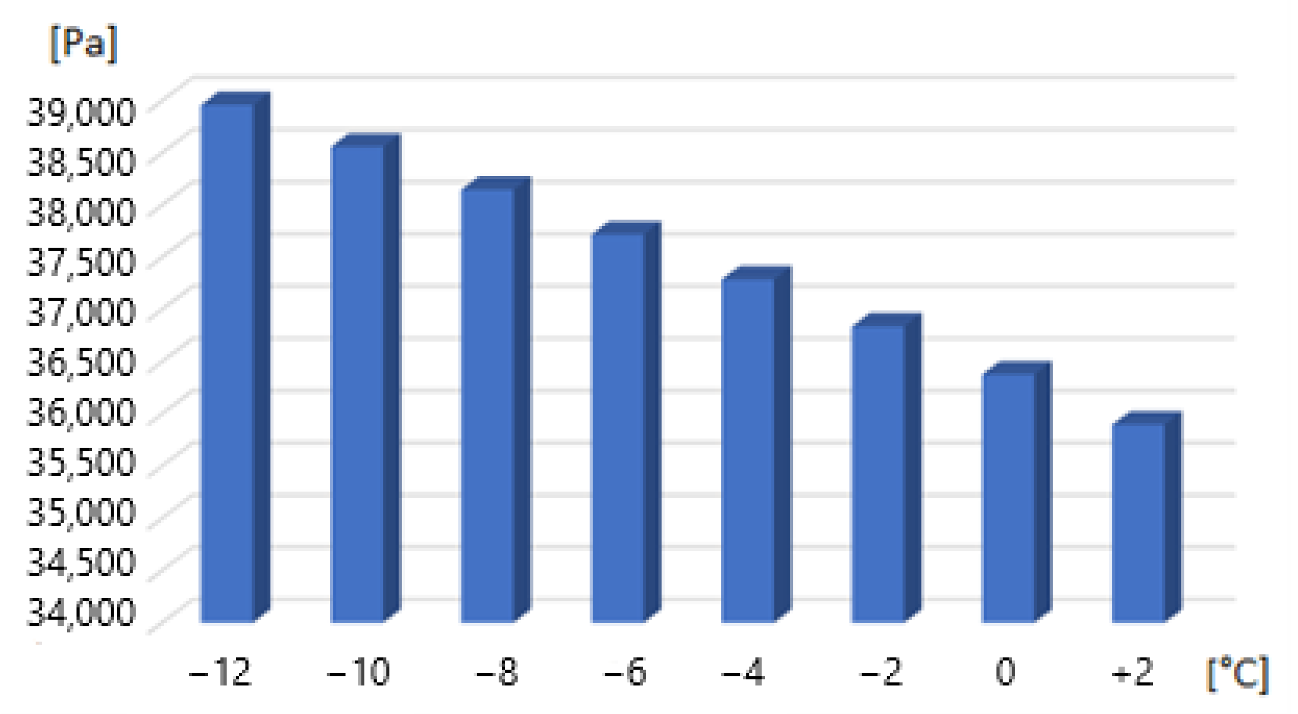
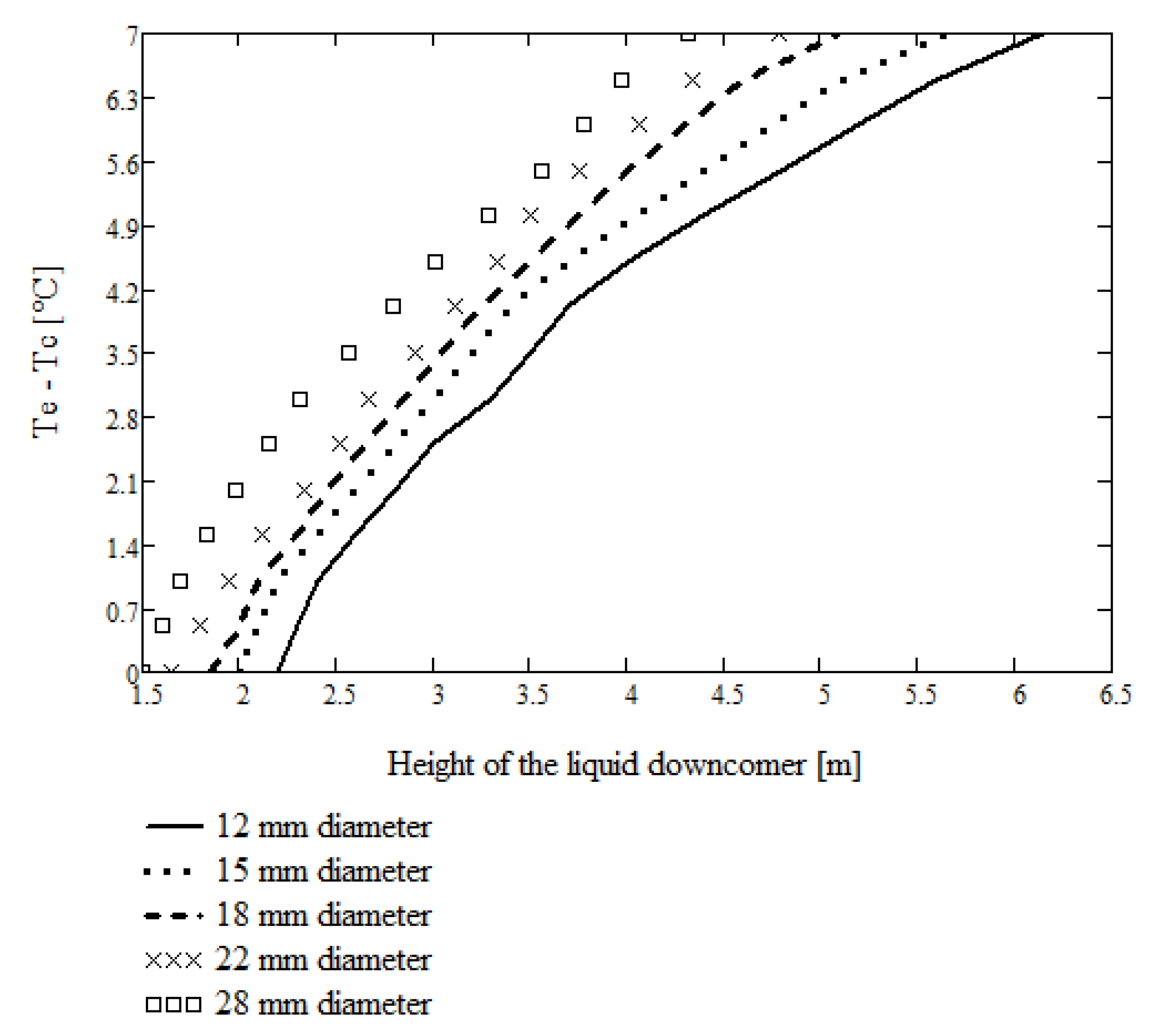
• It has been shown that as the mass flux of CO₂ as a working fluid increases, the temperature difference between evaporation and condensation increases, and it becomes necessary to increase the height of the liquid downcomer or increase the diameter of the pipeline.
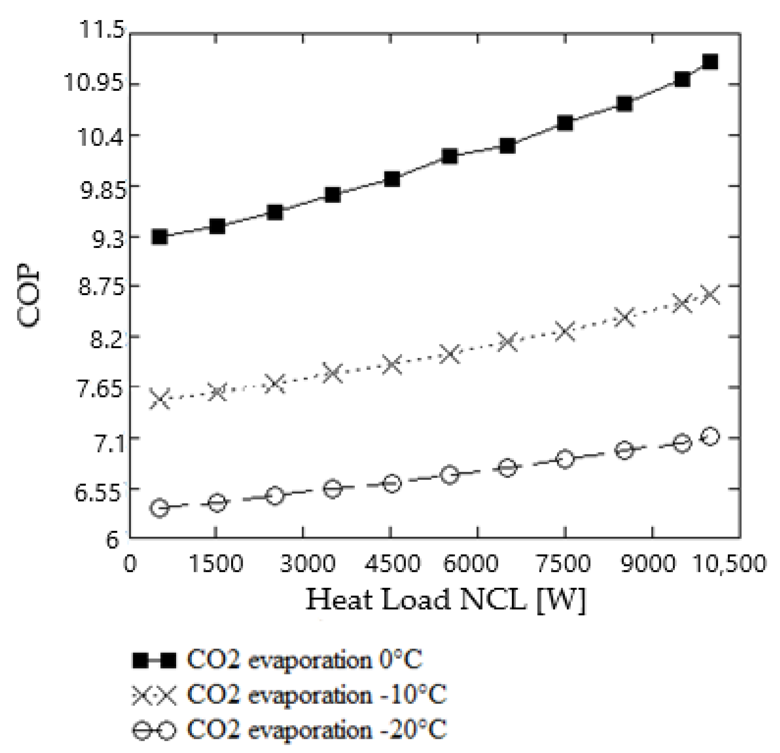
• The effect of a change in the refrigeration capacity of the circulating loop on the COP level of the coupled propane compressor refrigeration system was analysed for the first time. The highest COP was obtained for a CO₂ evaporation temperature of 0 °C; then, the COP value was 9.3 for a thermal capacity of 0.5 kW and 11.2 for a thermal capacity of 10 kW. An up to 23% increase in system efficiency was found as the refrigeration capacity of the system increases. Therefore, operation of the indirect refrigeration system with a CO₂ circulation loop should be avoided with a reduced refrigeration capacity.
• Raising the evaporation CO₂ temperature in the circulation loop from −20 °C to 0 °C improves the COP of the entire indirect refrigeration system by about 50%. This is of significant importance in terms of the applicability of such systems.

References

1. United Nation. Kigali Amendment to the Montreal Protocol on Substances that Deplete the Ozone Layer; Miscellaneous Series No. 2; United Nation: New York, NY, USA, 2016.
2. Polonara, F.; Kuijpers, L.; Peixoto, R. Potential impacts of the Montreal Protocol in Kigali Amendment to the choice of refrigerant alternatives. Int. J. Heat Technol. 2017, 35, S1–S8. [Google Scholar] [CrossRef]
3. Purohit, P.; Borgford-Parnell, N.; Klimont, Z.; Höglund-Isaksson, L. Achieving Paris climate goals calls for increasing ambition of the Kigali Amendment. Nat. Clim. Change 2022, 12, 339–342. [Google Scholar] [CrossRef]
4. Al-Joboory, H.N.S. Experimental investigation of gravity-assisted wickless heat pipes (thermosyphons) at low heat inputs for solar application. Arch. Thermodyn. 2020, 41, 257–276. [Google Scholar]
5. Allouhi, A.; Benzakour Amine, M.; Buker, M.S.; Kousksou, T.; Jamil, A. Forced-circulation solar water heating system using heat pipe-flat plate collectors: Energy and exergy analysis. Energy 2019, 180, 429–443. [Google Scholar] [CrossRef]
6. Karampour, M.; Sawalha, S. State-of-the-Art Integrated CO2 Refrigeration System for Supermarkets: A Comparative Analysis. Int. J. Refrig. 2018, 86, 239–257. [Google Scholar] [CrossRef] [Green Version]
7. Nisrene, M.A.; Puzhen, G.; Solomon, B. Natural circulation systems in nuclear reactors: Advantages and challenges. IOP Conf. Ser. Earth Environ. Sci. 2020, 467, 012077. [Google Scholar]
8. Wang, S.; Lin, U.C.; Wang, G.; Ishii, M. Experimental investigation on flashing-induced flow instability in a natural circulation scaled-down test facility. Ann. Nucl. Energy 2022, 171, 109023. [Google Scholar] [CrossRef]
9. Bieliński, H.; Mikielewicz, J. Application of a two-phase thermosyphon loop with minichannels and a minipump in computer cooling. Arch. Thermodyn. 2016, 37, 3–16. [Google Scholar] [CrossRef] [Green Version]
10. Tong, Z.; Zang, G. Effect of the diameter of riser and downcomer on an CO2 thermosyphon loop used in data centre. Appl. Therm. Eng. 2021, 182, 116101. [Google Scholar] [CrossRef]
11. Usman, H.; Ali, H.M.; Arshad, A.; Ashraf, M.J.; Khushnood, S.; Janjua, M.M.; Kazi, S.N. An experimental study of pcm based finned and un-finned heat sinks for passive cooling of electronics. Heat Mass Transf. 2018, 54, 3587. [Google Scholar] [CrossRef]
12. Zhang, X.W.; Niu, X.D.; Yamaguchi, H.; Iwamoto, Y. Study on a supercritical CO2 solar water heater system induced by the natural circulation. Adv. Mech. Eng. 2018, 10, 1–15. [Google Scholar] [CrossRef]
13. Amaya, A.; Scherer, J.; Muir, J.; Patel, M.; Higgins, B. GreenFire Energy Closed-Loop Geothermal Demonstration using Supercritical Carbon Dioxide as Working Fluid. In Proceedings of the 45th Workshop on Geothermal Reservoir Engineering, Stanford, CA, USA, 10–12 February 2020. [Google Scholar]
14. Baek, S.; Jung, Y.; Cho, K. Cryogenic two-phase natural circulation loop. Cryogenics 2020, 111, 103188. [Google Scholar] [CrossRef]
15. Cobanoglu, N.; Dogacan Koca, H.; Mete Genc, A.; Haktan Karadeniz, Z.; Ekren, O. Investigation of Performance Improvement of a Household Freezer by Using Natural Circulation Loop. Sci. Technol. Built Environ. 2021, 27, 85–97. [Google Scholar] [CrossRef]
16. Kumar, A.; Khalid, S. CO2 Based Natural Circulation Loops for Domestic Refrigerators. Saudi J. Eng. Technol. 2019, 4, 192–200. [Google Scholar]
17. Andrzejczyk, R.; Muszyński, T. The performance of H2O, R134a, SES36, ethanol, and HFE7100 two-phase closed thermosyphons for varying operating parameters and geometry. Arch. Thermodyn. 2017, 38, 3–21. [Google Scholar] [CrossRef] [Green Version]
18. Bai, Y.; Wang, L.; Zhang, S.; Lin, X.; Peng, L.; Chen, H. Characteristic map of working mediums in closed loop two-phase thermosyphon: Thermal resistance and pressure. Appl. Therm. Eng. 2020, 174, 115308. [Google Scholar] [CrossRef]
19. Thippeswamy, L.R.; Kumar, Y.A. Heat transfer enhancement using CO2 in a natural circulation loop. Sci. Rep. 2020, 10, 1507. [Google Scholar] [CrossRef] [PubMed] [Green Version]
20. Zhao, X.; Liu, S.; Huang, Y. Analysis of Heat Transfer Deterioration and Natural Circulation Flow Characteristics of Supercritical Carbon Dioxide in A Simple Circulation Loop. 2022. Available online: https://ssrn.com/abstract=4171532 (accessed on 10 July 2022).
21. Deng, B.; Chen, L.; Zhang, X.; Jin, L. The flow transition characteristics of supercritical CO2 based closed natural circulation loop (NCL) system. Ann. Nucl. Energy 2019, 132, 134–148. [Google Scholar] [CrossRef]
22. Wahidi, T.; Arunachala Chandavar, R.; Kumar Yadav, A. Supercritical CO2 flow instability in natural circulation loop: CFD analysis. Ann. Nucl. Energy 2021, 160, 108374. [Google Scholar] [CrossRef]
23. Thimmaimah, S.; Wahidi, T.; Yadav, A.; Arun, M. Comparative computational appraisal of supercritical CO2-based natural circulation loop: Effect of heat-exchanger and isothermal wall. J. Therm. Anal. Calorim. 2020, 141, 2219–2229. [Google Scholar] [CrossRef]
24. Thimmaimah, S.; Wahidi, T.; Yadav, A.; Arun, M. Numerical Instability Assessment of Natural Circulation Loop Subjected to Different Heating Conditions. In Recent Trends in Fluid Dynamics Research; Springer: Berlin/Heidelberg, Germany, 2022; pp. 249–262. [Google Scholar]
25. Bai, Y.; Wang, L.; Zhang, S.; Lin, X.; Peng, L.; Chen, H. Numerical analysis of a closed loop two-phase thermosyphon under states of single-phase, two-phase, and supercritical. Int. J. Heat Mass Flow Transf. 2019, 135, 354–367. [Google Scholar] [CrossRef]
26. Zhang, P.; Shi, W.; Li, X.; Wang, B.; Zhang, G. A performance evaluation index for two-phase thermosyphon loop used in HVAC systems. Appl. Therm. Eng. 2017, 17, 11577. [Google Scholar] [CrossRef]
27. Zhang, P.; Yang, X.; Rong, X.; Zhang, D. Simulation on the thermal performance of two-phase thermosyphon loop with large height difference. Appl. Therm. Eng. 2019, 163, 114327. [Google Scholar] [CrossRef]
28. Tong, Z.; Liu, X.H.; Jiang, Y. Three typical operating states of an R744 two-phase thermosyphon loop. Appl. Energy 2017, 206, 181–192. [Google Scholar] [CrossRef]
29. Saikiran, A.P.; Banoth, P.; Maddali, R. Dynamic model of supercritical CO2 based natural circulation loops with fixed charge. Appl. Therm. Eng. 2020, 169, 114906. [Google Scholar]
30. Tong, Z.; Liu, X.H.; Jiang, Y. Experimental study of the self-regulating performance of an R744 two-phase thermosyphon loop. Appl. Energy 2017, 186, 1–12. [Google Scholar] [CrossRef]
31. Würfel, R.; Ostrowski, N. Experimental investigations of heat transfer and pressure drop during the condensation process within plate heat exchangers of the herringbone-type. Int. J. Therm. Sci. 2004, 24, 59–68. [Google Scholar] [CrossRef]
32. McDonough, J.M. Lectures in Elementary Fluid Dynamics: Physics, Mathematics and Applications; University of Kentucky: Lexington, KY, USA, 2004. [Google Scholar]
33. Thome, J.R.; El Hajal, J. Two-phase flow pattern map for evaporation in horizontal tubes: Latest version. In Proceedings of the First International Conference on Heat Transfer, Fluid Mechanics and Thermodynamics, Kruger Park, South Africa, 8–10 April 2002; pp. 182–188. [Google Scholar]
34. Cheng, L.; Ribatski, G.; Quiben, J.M.; Thome, J.R. New prediction methods for CO2 evaporation inside tubes: Part I—A two-phase flow pattern map and a flow pattern based phenomenological model for two-phase flow frictional pressure drops. Int. J. Heat Mass Transf. 2008, 51, 111–124. [Google Scholar] [CrossRef]
35. Kattan, N.; Thome, J.R.; Favrat, D. Flow boiling in horizontal tubes. Part 1: Development of a diabatic two-phase flow pattern map. J. Heat Transf. 1998, 120, 140–147. [Google Scholar] [CrossRef]
36. Wojtan, L.; Ursenbacher, T.; Thome, J.R. Investigation of flow boiling in horizontal tubes: Part I—A new diabatic two-phase flow pattern map. Int. J. Heat Mass Transf. 2005, 48, 2955–2969. [Google Scholar] [CrossRef]
37. Schmid, D.; Verlaat, B.; Petagna, P.; Revellin, R.; Schiffmann, J. Flow pattern observations and flow pattern map for adiabatic two-phase flow of carbon dioxide in vertical upward and downward direction. Exp. Therm. Fluid Sci. 2022, 131, 110526. [Google Scholar] [CrossRef]
38. Hsieh, Y.Y.; Lin, T.F. Saturated flow boiling heat transfer and pressure drop of refrigerant R-410A flow in a vertical plate heat exchanger. Int. J. Heat Mass Transf. 2002, 45, 1033–1044. [Google Scholar] [CrossRef]
39. Quiben, J.M.; Thome, J.R. Flow pattern based two-phase frictional pressure drop model for horizontal tubes. Part I: Diabatic and adiabatic experimental study. Int. J. Heat Fluid Flow 2007, 28, 1060–1072. [Google Scholar] [CrossRef]
40. Park, C.Y.; Hrnjak, P.S. CO2 and R410A flow boiling heat transfer, pressure drop, and flow pattern at low temperatures in a horizontal smooth tube. Int. J. Refrig. 2007, 30, 166–178. [Google Scholar] [CrossRef]
41. Flack, K.A.; Shultz, M.P. Roughness effects on wall-bounded turbulent flows. Phys. Fluids 2014, 26, 101305. [Google Scholar] [CrossRef] [Green Version]
42. Incropera, F.P.; DeWitt, D.P.; Bergman, T.L.; Lavine, A.S. Fundamentals of Heat and Mass Transfer, 6th ed.; Wiley: New York, NY, USA, 2006. [Google Scholar]
43. Gasche, J.L. Carbon dioxide evaporation in a single micro-channel. J. Braz. Soc. Mech. Sci. Eng. 2006, 28, 69–83. [Google Scholar] [CrossRef]
44. Ozawa, M.; Ami, T.; Ishihara, I.; Umekawa, H.; Matsumo, R.; Tanaka, Y.; Yamamoto, T.; Ueda, Y. Flow pattern and boiling heat transfer of CO2 in horizontal small-bore tubes. Int. J. Multiph. Flow 2009, 35, 699–709. [Google Scholar] [CrossRef]
45. Mitrovic, J. Heat Exchangers—Basics Design Application; IntechOpen: London, UK, 2012. [Google Scholar]
46. Yang, X.; Zhang, P.; Li, Y.; Zhang, D. A practical design method for two-phase thermosyphon loop based on approaching degree to “ideal cycle”. Appl. Therm. Eng. 2021, 182, 116059. [Google Scholar] [CrossRef]
47. Khodabandeh, R. Heat transfer in the evaporator of an advanced two-phase thermosyphon loop. Int. J. Refrig. 2005, 28, 190–202. [Google Scholar] [CrossRef]
Figure 1. Schematic of the analysed indirect cooling system with CO2 NCL: 1. propane chiller (R290); 2. plate heat exchanger as evaporator in the propane cycle and condenser in the CO 2 circulation loop; 3. CO 2 tank; 4. CO 2 evaporator; ∆H—height of the liquid downcomer.
Sustainability 14 10422 g001
Figure 2. Schematic of channel section in two-phase separated flow: D—internal channel diameter: h l —height when filling the channel with liquid; P i —the ratio of the length of the fluid interface to the fill height in the channel; A l —liquid phase area; P l —perimeter of tube wetted by liquid; A v —vapour phase surface cross-section area; P v —pipe circuit in contact with vapour phase; θ m —wet angle of the tube perimeter; θ s —dry angle of the tube perimeter.
Sustainability 14 10422 g002
Figure 3. CO2 two-phase flow pattern map based on own prediction: A—annular flow; D—dry-out region; I—intermittent flow; M—misty flow; S—tratified flow; SLUG—slug flow; SW—stratified-wavy flow; The experimental data observed by Gasche [43]: 1,2—slug flow; 3—slug/annular flow; 4,5—annular flow.
Sustainability 14 10422 g003
Figure 4. CO2 two-phase flow pattern map based on own prediction, where: A—annular flow; D—dry-out region; I—intermittent flow; M—misty flow; S—stratified flow; SLUG—slug flow; SW—stratified-wavy flow. The experimental data observed by Ozawa et al. [44]: 1—bubbly flow; 2—slug/annular flow; 3—annular flow; 4—misty flow; 5—plug flow; 6—slug flow; 7—annular flow; 8—misty flow.
Sustainability 14 10422 g004
Figure 5. Operation parameters of the NCL in the experimental investigations, acc. to [10].
Sustainability 14 10422 g005
Figure 6. Predicted hydrostatic pressure of the column of liquid at the loop of height of 4 m for various condensation temperatures.
Sustainability 14 10422 g006
Figure 7. Height of the liquid downcomer with respect to temperature difference.
Sustainability 14 10422 g007
Figure 8. Effect of heat load on mass flux and required temperature difference between condenser and evaporator.
Sustainability 14 10422 g008
Figure 9. Schematic diagram of propane refrigeration unit equipped with a CO2 circulation loop: 1—propane condenser with fan; 2—expansion valve; 3—plate heat exchanger as evaporator in the propane cycle and condenser in the CO 2 circulation loop; 4—compressor; 5— CO 2 tank; 6— CO 2 evaporator.
Sustainability 14 10422 g009
Figure 10. Effect of CO2 evaporation temperature and heat load of NCL on COP of propane refrigeration unit.
Sustainability 14 10422 g010