Article

Hysteresis Behavior Modeling of Hard Rock Based on the Mechanism and Relevant Characteristics

1
School of Civil Engineering, Central South University, Changsha 410075, China
2
National Engineering Laboratory for High Speed Railway Construction, Central South University, Changsha 410075, China
3
China Railway First Survey and Design Institute Group Co., Ltd., Xi’an 710043, China
*
Author to whom correspondence should be addressed.
Sustainability 2022, 14(16), 10412; https://doi.org/10.3390/su141610412
Submission received: 13 July 2022 / Revised: 15 August 2022 / Accepted: 17 August 2022 / Published: 22 August 2022
(This article belongs to the Section Sustainable Engineering and Science)

Abstract

:
The modeling of cyclic behavior in rock remains a challenge due to complex deformation characteristics. This paper studied the mechanical behaviors of granite samples under uniaxial cyclic loading and unloading through cyclic compression tests and acoustic emission (AE) monitoring. Then, a comprehensive body that consisted of an elastic element, plastic element, and friction element was proposed to describe the stress–strain relationship with respect to cyclic behavior, in which the friction element was connected in parallel with the serial combination of the elastic element and plastic element. Finally, the parameters of the proposed model were calibrated based on the mechanism analysis and backpropagation (BP) neural network. Results show that the behavior during unloading is primarily elastic and is accompanied by the obstruction of friction. During reloading, the behavior changes from elastic to elastic–plastic before and after the Kaiser point. The tangential modulus of the elastic element is dynamic in a linear positive correlation with elastic strain and a linear negative correlation with plastic strain; specifically, the elastic strain controls the variation process of the elastic modulus while the plastic strain determines the lower limit. The constitutive law of the plastic element is expressed by a logistic function, which means that the plastic strain increases in a trend of acceleration–deceleration. The friction element plays a major role in processing the massing effect, and the plastic element is prompted before the historical maximum stress, which reflects the ratcheting effect and Felicity effect. The reliability of the proposed constitutive model is confirmed by the comparison of the simulated stress–strain curves with the experimental curves.

1. Introduction

In the field of underground engineering, many projects may face cyclic loading compression, for example, the deep reservoirs for fuel storage or gas storage, hydraulic tunnels, and so on [1,2,3]. In addition, some studies have been conducted using cyclic loading and unloading experiments, such as energy analysis in rock bursts [4]. The deformation characteristics and corresponding constitutive model available to represent these characteristics are important for rock engineering projects that are subjected to cyclic compression.
There are some differences in the strength and deformation characteristics between cyclic loading and monotonic loading for rock. Generally, the strength of rock under cyclic loading is marginally smaller than that under monotonic loading [5], and the stress–strain relation under cyclic compression exhibits a peculiar massing effect and ratcheting effect. There are two explanations for the massing effect or hysteresis: elastic energy dissipation resulting from friction or stick-slip between the inner fissures [6]; and hysteresis due to the phase difference between the stress and strain [7], which could be suitable for rock subjected to cyclic loading with a relatively high frequency. These two explanations may be correlative; with the development of rock damage, the fissures extend and coalesce, which results in more energy dissipation and phase difference. In order to quantify the damage or degradation of rock under cyclic loading, some indices have been presented, such as the area of the hysteretic loop [8] and the intersection angle of the X-shaped tangent modulus in one cycle [9]. Both values increase with the number of cycles, which indicates the deterioration of the rock. In addition, Meng et al. [10,11] used the acoustic emission (AE) method to measure the degradation of rock in each cycle and found a strong AE phenomenon when the reloading level exceeded the peak stress of the last cycle, and the phenomenon occurred in advance to some degree when loading approximated the uniaxial compressive strength (UCS) (i.e., the Felicity effect). Therefore, the Felicity ratio is also considered an index to evaluate the degradation of rock [12], and the variation is similar to the aforementioned indices.
A rational constitutive model is supposed to represent the deformation characteristics. The general elastic–plastic models have difficulty when describing the massing effect and ratcheting effect due to complex stress paths; thus, researchers have developed some statistical approaches [13] or modified constitutive models to simulate the cyclic behavior. The Preisach–Mayergoyz (PM) model was developed by McCall and Guyer [14], who believed that hysteretic behavior arose from mesoscopic structural features; thus, the material was considered to consist of enormous hysteretic mesoscopic elastic units (HMEUs). These units can describe nonlinear elastic behavior and hysteretic behavior in conjunction with effective medium theory. Scalerandi et al. [15] used the PM model to implement the adhesion mechanism with three elastic states, and the effect of three proposed geometric constraints of PM space and transition parameters on nonlinear response were also discussed. Chen et al. [16] performed uniaxial cyclic tension tests with different frequencies and improved the PM model by introducing two attenuation coefficients into the density function of HMEU so that the loading frequency could be considered. Wang et al. [17] developed a modified PM model by substituting the HMEU with a generalized Kelvin body to introduce creep characteristics. Hua and Jiang [18] extended the traditional PM model to the three-dimensional case by introducing initial closed HMEUs and the direction of each HMEU. The PM model performs well in hysteretic characteristics, but for the case of equal amplitude cyclic loading and unloading, the ratcheting effect and the Felicity effect cannot be completely addressed. In addition to the PM model, the subloading surface model [19,20,21] is another typical approach to simulate cyclic behavior. In this theory, plastic deformation could occur, although the stress situation is inside the yield surface; thus, the transition from elasticity to plasticity is smooth. Zhou et al. [22,23] selected the modified Drucker–Prager criterion as the appropriate yield surface for rock material and then incorporated the cohesion weakening and frictional strengthening model into the subloading surface theory to reflect the degradation of the strength and failure of rock. The subloading surface model is capable of describing the massing effect and ratcheting effect under cyclic loading; however, the plastic deformation that occurs during unloading is beyond the physical understanding, and the Felicity effect is also neglected. Furthermore, there are also other models, such as the endochronic theory [24] and the bounding surface model [25]; however, their application is limited due to the relative complexity of the model and the difficulty of calibrating many parameters.
In summary, previous studies regarding the cyclic mechanical behavior modeling of rock only reflect parts of stress–strain curve characteristics. However, each characteristic plays a respective role in the whole cyclic loading and unloading process, the massing effect accounts for basic hysteresis features, the ratcheting effect induces the hysteretic loop to move forward, the Felicity effect causes the current hysteretic loop to evolve in a different trace from the last loop, and the damage of rock results in the variation of tangential modulus in terms of the stress–strain curve. The lack of any characteristic will make the simulated curve deviate from the experimental curve, and the modeling of cyclic mechanical behavior considering all characteristics still remains incompletely resolved.
The goal of this study is to develop a constitutive model that sufficiently reflects rock’s cyclic characteristics, including the massing effect, ratcheting effect, Felicity effect, and influence of damage; moreover, it is better for this model to comply with physical understanding. First, the mechanical behavior of granite samples under cyclic loading and unloading was investigated by integrating a compression test with AE monitoring. Second, a comprehensive body consisting of an elastic element, plastic element, and friction element was presented; the corresponding constitutive laws were proposed based on the deformation characteristics; and an algorithm that simulated the actual stress–strain curve was introduced. Finally, relevant parameters were calibrated based on the mechanism and BP neural network.

2. Experimental Foundation for the Constitutive Model

2.1. Rock Samples and Experimental Scheme

The uniaxial cyclic loading and unloading experiments are performed first. The lithology of the rock samples is granite, which comes from the Gangdese Orogenic Belt in eastern Tibet Province, China. The mineral composition and concentration of rock samples are presented in Table 1, and some physical and mechanical parameters are determined via indoor testing, as presented in Table 2. Three tested samples are processed to the standard cylinder with a height of 100 mm and diameter of 50 mm, and all samples are ensured to have good integrity.
Cyclic loading is provided by a microcomputer-controlled electrohydraulic servo facility, and the axial strain is measured by a strain gauge. In addition, the AE signal generated during testing is collected by a holographic acoustic emission signal acquisition system with two channels. Although two AE sensors seem to be insufficient to locate the source of AE events, the requirement for capturing the damage occasions is still satisfied, and the two AE sensors are placed on the middle part of the rock sample symmetrically (Figure 1) so as to monitor the entire specimen comprehensively. In this experiment, the rock samples are subjected to cyclic loading and unloading eight times, and the peak stress of each cycle is 5, 15, 35, 45, 55, 90, 100, and 125 MPa. The stress is released once it reaches the designed peak stress, and then the next cycle begins. In each cycle, the loading and unloading processes were performed in a strain-controlled mode. In this study, three conditions of different loading rates vl (0.6, 0.9, and 1.2 mm/min) were designed, and the unloading rate was uniformly set to 0.9 mm/min. After 8 cycles, loading monotonically increases until failure occurs.

2.2. Results and Analysis of Mechanical Behavior

The experimental stress–strain curve is shown in Figure 2. The envelope composed of each loading curve reveals four deformation stages of the rock sample (i.e., the compaction stage, elastic stage, yield stage, and post-peak stage), as reported in other published literature [11,26]. The transition from the elastic stage to the yield stage is unclear; in addition, the elastic strain and plastic strain always occur simultaneously no matter which stage the rock sample is in because the rock exhibits hysteresis throughout compression.
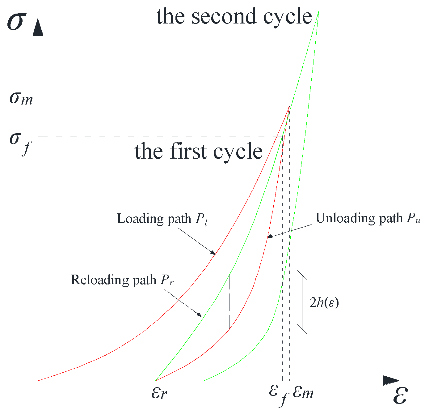
The variation in AE hits monitored throughout the test is shown in Figure 3. The AE signal is a kind of elastic stress wave released by materials under external disturbance; in terms of rock materials, the signal mainly results from the formation and propagation of cracks in addition to a small part of signals due to the cracks’ compaction and friction. Therefore, the AE signal can be regarded as a representation of crack development; furthermore, considering that damage to rock samples is closely related to the crack evolution, some researchers used AE parameters to reflect the damage degree of rock and proposed a damage variation based on AE counts [27,28]. In Figure 3, the AE signal remains silent (below 10 per second) most of the time in one cycle but will actively increase dozens of times more than before while the increasing stress level approaches the peak stress of the last cycle; the mutation moment (Kaiser point) is denoted by vertical dashed lines in Figure 3. It is noted that the stress σf that prompts numerous AE signals is always below the peak stress σm of the last cycle (i.e., the Felicity effect), and the schematic relationship is shown in Figure 4.
The marked differences in the AE phenomenon before and after σf imply that the mechanical behaviors are different. When stress is on the unloading path Pu and the reloading path Pr before σf, the AE signal is minimal because the source is the friction between inner fissures or cracks. However, when the reloading stress exceeds σf, new plastic damage occurs, which will result in numerous AE signals.
With regard to the AE quiet period (σmi−1→ 0→ σ   f i , where i represents the number of cycles), the energy variation is primarily attributed to the release and accumulation of elastic energy. In this paper, the elastic stress is noted as f(ε), and friction is noted as h(ε). Then, the stress on Pu can be expressed as f(ε) − h(ε) because Pu is a process in which a rock sample performs work to the outside, and some energy is consumed by the friction of inner cracks. In contrast, the stress on Pr can be expressed as f(ε) + h(ε) because the facility must overcome friction and perform work on the rock sample. As a result, Pr is over Pu with a difference of 2 h(ε), which could explain the massing effect to a certain extent.
With regard to the AE active period (σ   f i σmi), the new plastic deformation begins to develop before the stress reaches σmi−1 due to the Felicity effect. Therefore, the loading path Pli will not extend along the trend of Pli−1 completely but will enter the elastic–plastic stage in advance, which could explain the ratcheting effect to some extent.

3. Constitutive Model and Relative Numerical Implementation

3.1. Basic Hypothesis

Based on mechanism analysis, several hypotheses are presented as follows:
(a)
The elastic deformation and plastic deformation occur simultaneously during the initial loading and the reloading process from σ   f i to σmi for the subsequent cycles.
(b)
Only elastic deformation occurs during unloading and reloading from 0 to σ   f i for each cycle.
(c)
The value of friction is dominated by roughness and contact pressure between surfaces in general; in this study, these two factors are considered to be representative of plastic deformation (damage degree of rock sample) and stress level, respectively. Therefore, the greater the damage and stress are, the greater the friction. In addition, friction performs negative work to the facility during the loading process but performs negative work on the rock sample during the unloading process.

3.2. Constitutive Model

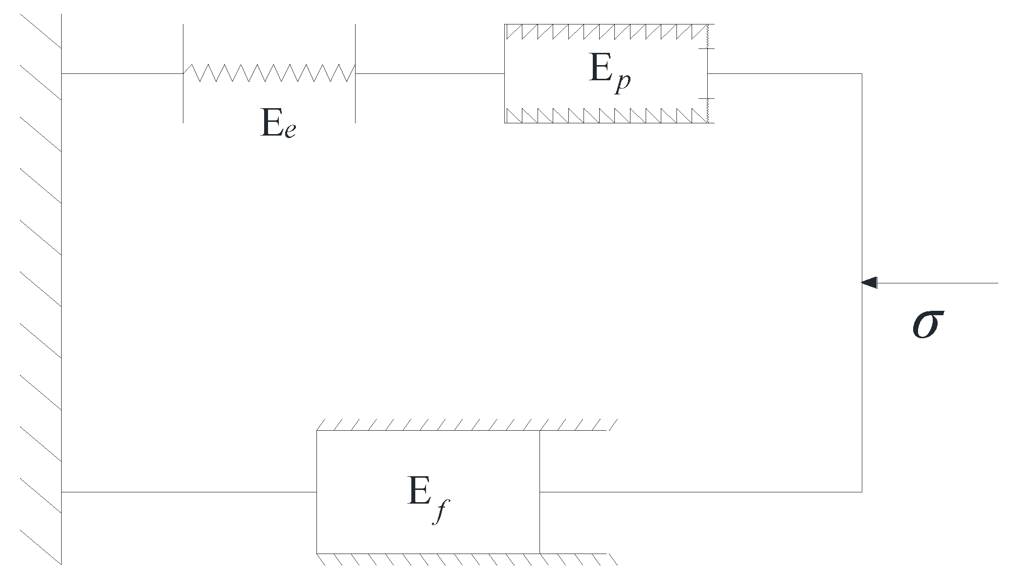
The constitutive body is composed of three varied elements: the elastic element Ee, plastic element Ep, and friction element Ef. The elastic and plastic elements are connected in series, and this assembly is connected with the friction element in parallel, as shown in Figure 5.
The stress of Ee is only related to the elastic deformation εe and is noted as f(εe). The stress of Ep is related to the accumulated plastic deformation εp and is noted as g(εp), and εp is irreversible. The friction of Ef is related to εp and the stress level, in which the latter can be reflected by f(εe) for simplicity; thus, the value of friction is noted as h(εp, f).
For the case of the loading process from σ   f i to σmi (when i = 1, σ   f i = 0), the correlation laws of stress and strain between elements are given as Equation (1):
{ f ( ε e ) = g ( ε p ) ε = ε e + ε p σ = f ( ε e ) + h ( ε p ,   f )
For the case of the unloading process from σmi to 0, the correlation laws of stress and strain between elements are given as Equation (2):
{ ε p   remain   unchanged   ε = ε e + ε p σ = f ( ε e ) h ( ε p ,   f )
For the case of the reloading process from 0 to σfi+1, the correlation laws of stress and strain between elements are given as Equation (3):
{ ε p   remain   unchanged   ε = ε e + ε p σ = f ( ε e ) + h ( ε p ,   f )

3.3. Procedure of Computer Implementation

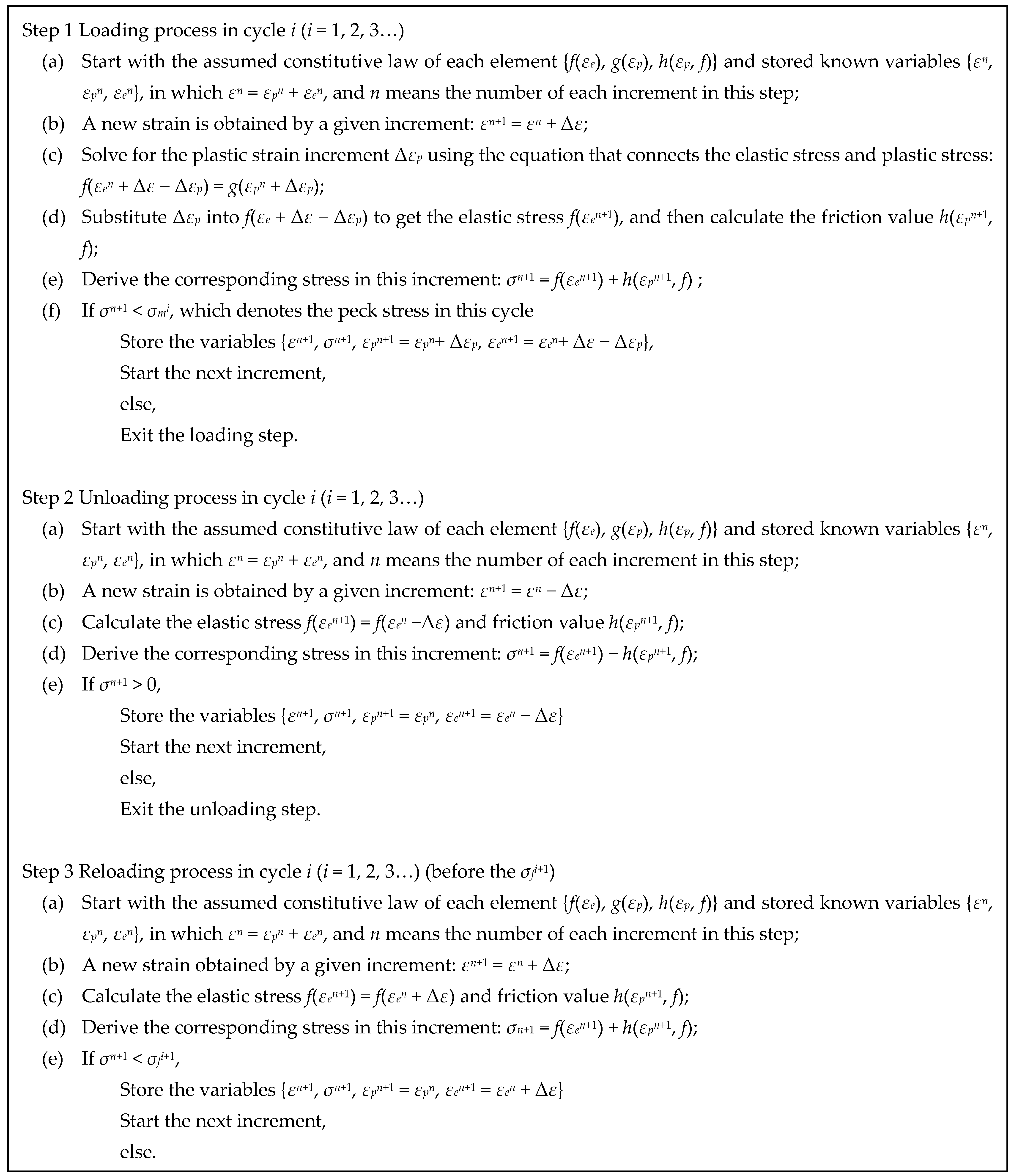
For each cycle, the implementation procedure can be divided into three steps: loading, unloading, and reloading. Every step is driven by strain increment Δε until the respective stress threshold is reached. The procedure is specified in Figure 6.

3.4. Constitutive Law of Elements in the Proposed Model

3.4.1. Determination of f(εe)

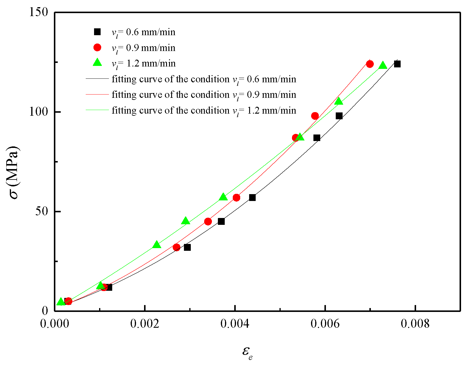
In theory, the elastic element’s constitutive law f(εe) is linear, but this linear relationship can hardly coincide well with the experimental curves of the rock sample. In reality, the tangential modulus always varies due to the tight or loose state of microscopic particles and damage development. Here, the constitutive law fl(εe) of Ee during loading (AE active period) is considered first, which is explored by extracting the elastic strain εe (or recoverable strain) of the peak point in each cycle, as shown in Figure 7. The f(εe) for each condition is well fitted by a polynomial (Equation (4)), and the corresponding parameters are shown in Table 3. It reveals that the elasticity increases linearly with εe because the rock sample becomes denser during compression.
f l ( ε e ) = k 11 ε e + k 12 ε e 2
Compared with the loading process, the constitutive law of Ee for the unloading process may be different; relevant characteristics are validated by the experimental results in Figure 8, in which the abovementioned εe-σ trend (Figure 7) is compared with the stress–strain curve of each unloading path. The curves seem to be parallel in general, except for the ending of unloading curves, in which the trend becomes gentler with the number of cycles. This phenomenon results from the elasticity loss due to the degradation of the rock sample; when rock changes from a dense state to a loose state with the release of stress, the effect of damage becomes more marked. In other words, the elasticity variation is dominated by εe, while the damage controls the lower limit.
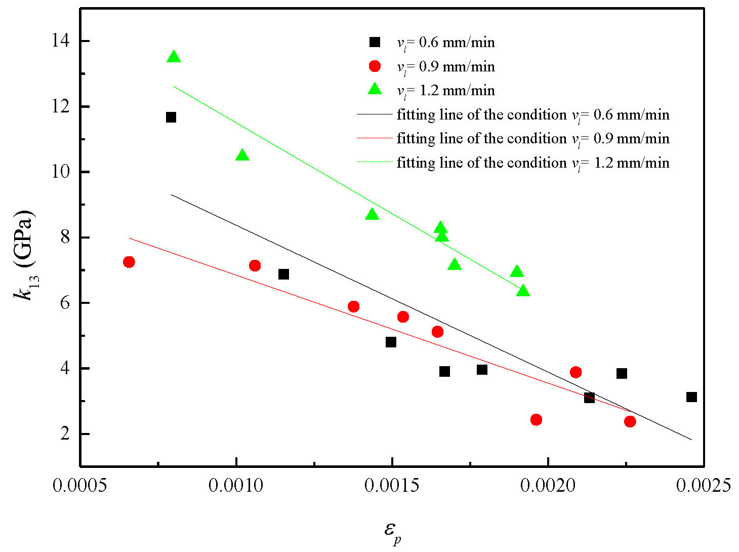
The residual strain εr can reflect the damage degree of the rock sample [29,30], and there is a one-to-one correspondence relation between the residual strain and deformation modulus [31]. This paper investigates the tangential modulus k13 at the endpoint of the unloading path in each cycle, at which the effect of accumulated plastic strain is sufficiently manifested. The value of k13 and the corresponding residual strain εr are plotted in Figure 9. It can be easily found that the tangential modulus decreases with the accumulation of plastic strain. This relationship can be approximately fitted by a linear equation (Equation (5)), and relevant parameters are derived by the regression method, as shown in Table 4.
k 13 = k 13 ε p + b 13
So as to explore the constitutive law fu(εe) of Ee for the unloading process, the gradient values of the entire unloading path are calculated and plotted in Figure 10; the gradient of the unloading path can be considered to be the derivative of fu(εe) with respect to εe approximately (i.e., fu′(εe)). In Figure 10, the relationship between fu′(εe) and ε is also fitted by a linear function, and the fitting effect is acceptable according to the high correlation coefficients. As a result, fu(εe) is considered a quadratic equation, which agrees with fl(εe); the equation can be determined by the peak point and trough point of each cycle. The relevant boundary conditions are depicted as Equation (6).
{ ε e i = ε m i ε r i ,   f u ( ε e i ) = σ m i ε e i = 0 ,   f u ( ε e i ) = k 13 ,   f u ( ε e i ) = 0
By substituting Equation (6) into the quadratic equation, the fu(εe) of Ee for the unloading process can be obtained as Equation (7). In addition, considering that the reloading process from 0 to σfi+1 is also in the AE quiet period, the deformation characteristic and mechanism are the same as the unloading process; thus, Equation (7) is also applicable to this process as the constitutive law of Ee. In summary, the constitutive law of Ee for the loading and unloading process can be incorporated as Equation (8).
f u ( ε e i ) = k 13 ε e i + σ m i k 13 ( ε m i ε r i ) ( ε m i ε r i ) 2 ( ε e i ) 2
f ( ε e ) = { k 11 ε e + k 12 ε e 2   ( step   1   in   Figure   6 ) k 13 ε e + σ m i k 13 ( ε m i ε r i ) ( ε m i ε r i ) 2 ( ε e ) 2   ( step   2   and   step   3   in   Figure   6 )

3.4.2. Determination of g(εp)

In order to deduce the expression of g(εp), a differential strain increment dε is considered first, and g(εp) in dε can be considered to be a linear segment. According to the series relationship between the elastic element and plastic element, the corresponding stress equation can be written as Equation (9), in which g’ denotes the derivatives with respect to εp; thus, the differential plastic strain increment p can be derived as Equation (10).
f ( ε e ) ( d ε d ε p ) = g d ε p
d ε p = f ( ε e ) d ε f ( ε e ) + g
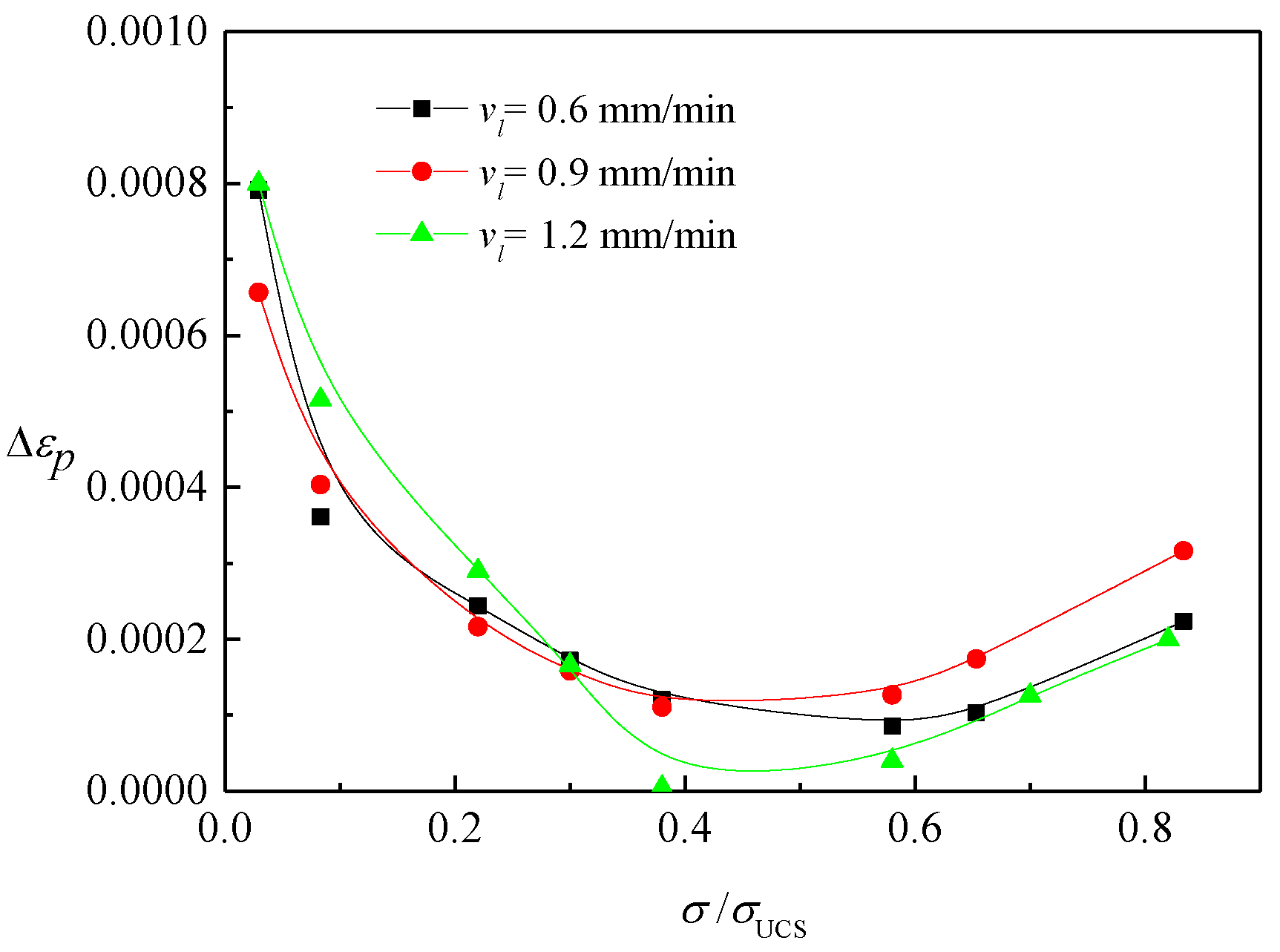
It can be seen that the gradient of g(εp) is inversely proportional to εp (i.e., the larger the gradient is, the smaller the plastic strain increment). This study extracted the plastic strain increment ∆εp in each cycle from the experimental data, and Figure 11 plotted ∆εp versus the ratio of peak stress to UCS σ/σUCS; here, the σ/σUCS was chosen due to the difference between rock samples. Figure 11 shows that ∆εp exhibits a decreasing–stable–increasing trend throughout the deformation process, which means that the plastic strain increases rapidly at the initial stage and then develops slowly for a certain duration. Finally, the increment accelerates gradually as the stress approaches UCS. Similar results were also found in other studies [32,33]; therefore, g(εp) was supposed to increase in a trend of acceleration–deceleration. In this study, the Logistic equation is used to describe g(εp) by referring to Liu et al. [26], and the equation is formulated as Equation (11), in which k2, a, and b are parameters that need to be predicted.
g ( ε p ) = k 2 1 + e a b ε p
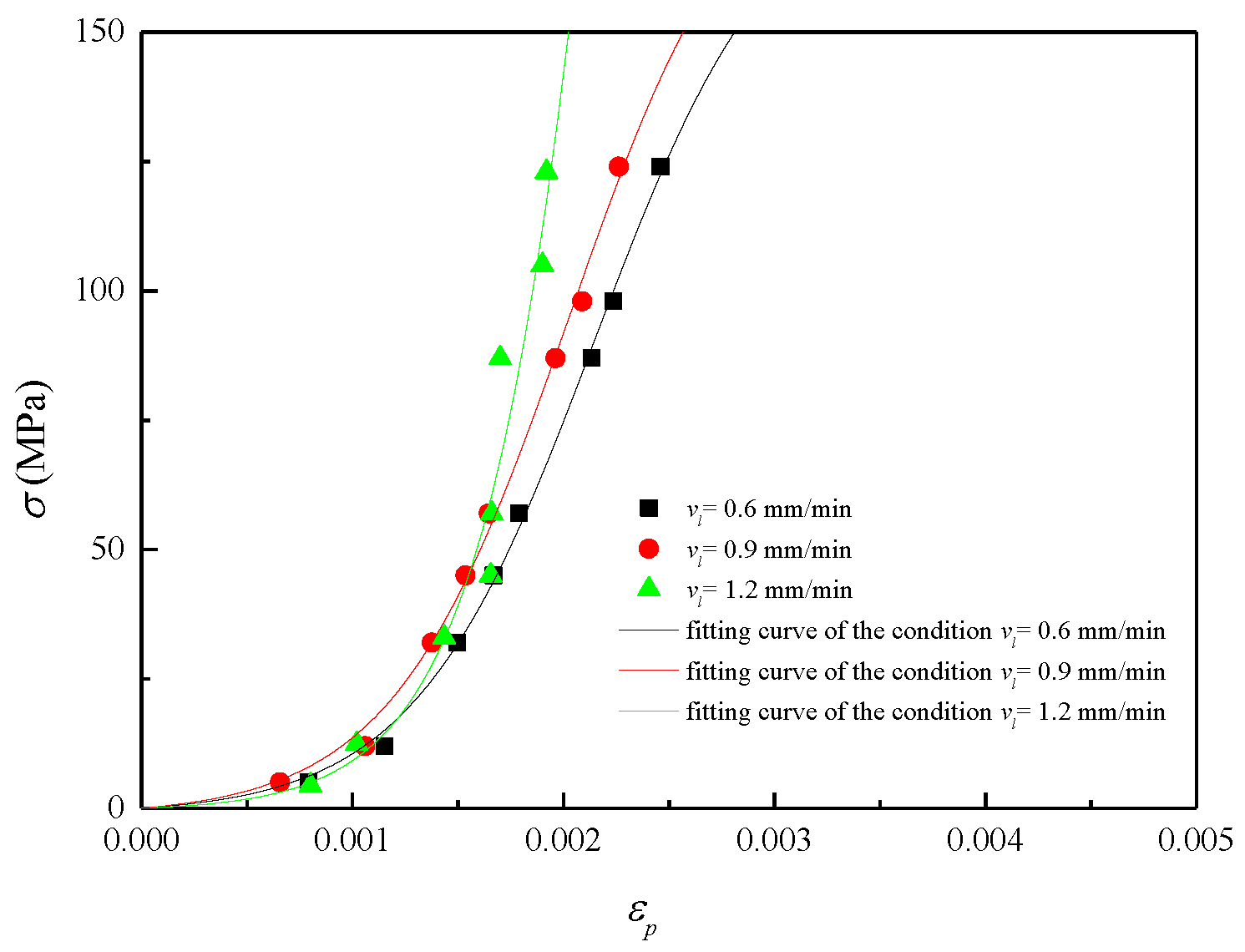
The plastic strain εp (i.e., residual strain) of the peak point in each cycle is extracted, and the relationship with stress is fitted by Equation (11) in Figure 12. The corresponding parameters are given in Table 5, in which the high goodness of fit values reveal that the fitting effect is satisfactory.
It should be noted that if Equation (11) is applied to each cycle directly, the reloading stress–strain curve will extend along the loading stress–strain curve of the last cycle completely, which means that the hardening will not be influenced by cyclic loading, and the ratcheting effect and Felicity effect disappear, as shown in Figure 13a, which is inconsistent with reality (Figure 13b). Therefore, a bias term ci is introduced to Equation (11), representing that the rock enters the yield state in advance when reloading for each cycle. The relationship between the stress and yield surface throughout the cyclic loading process is then schematically plotted in Figure 14. In this way, the ratcheting effect and Felicity effect can be easily reflected in the model; thus, Equation (11) is modified to Equation (12).
g ( ε p ) = k 2 1 + e a b ( ε p c i )
where ci is considered to be dominated by the historical maximum stress and rock strength, so it is expressed as Equation (13) for simplicity, where d is also a parameter to be predicted. In addition, the occasion of σfi is regarded as the Kaiser point, so the value is expressed as Equation (14), where RF is the Felicity ratio. The experimental values of RF for each cycle in different conditions are shown in Table 6, in which subtle changes are observed; the small difference in RF only causes a negligible effect on the entire posture of the stress–strain curve; thus, this paper simplifies RF as a constant equal to 0.95.
c i = d σ m i σ U C S
σ f i = R F σ m i 1

3.4.3. Determination of h(εp, f)

According to the mechanism analysis and relevant hypothesis, on the one hand, the roughness of contact surfaces is dominated by εp. More εp means more friction surface; thus, the roughness is simplified to be k31εp, where k31 is the coefficient. On the other hand, the pressure between the contact surfaces is dominated by f(εe), and higher f(εe) means that the contact is closer between surfaces. Thus, the pressure is simplified to be k32f, where k32 is also the coefficient. In summary, h(εp, f) is formulated as Equation (15), where k3 = k31k32, and also needs to be predicted in the following section.
h ( ε ) = k 3 ε p f

4. Parameter Calibration

4.1. Calibration Procedure

There are 9 parameters (k11, k12, k13′, b13′, k2, a, b, d, k3) that need to be determined. It is noted that although Table 3, Table 4 and Table 5 give the preliminary values of some parameters, these values are derived by decoupling the parameters; when the coupling effect is considered, the simulated results may deviate from the experimental curves. Therefore, this study uses the BP neural network to calibrate further the parameters. The neural network is a data-driven method that can simulate any nonlinear relationship in theory; however, too many parameters may make the neural network fall into the disaster of dimensionality. Fortunately, mechanism analysis can relieve the adverse effect of multiple parameters. In other words, the reference values in Table 3, Table 4 and Table 5 can help us narrow the number of parameters, as well as the range of parameter values, and create a superior sample set.
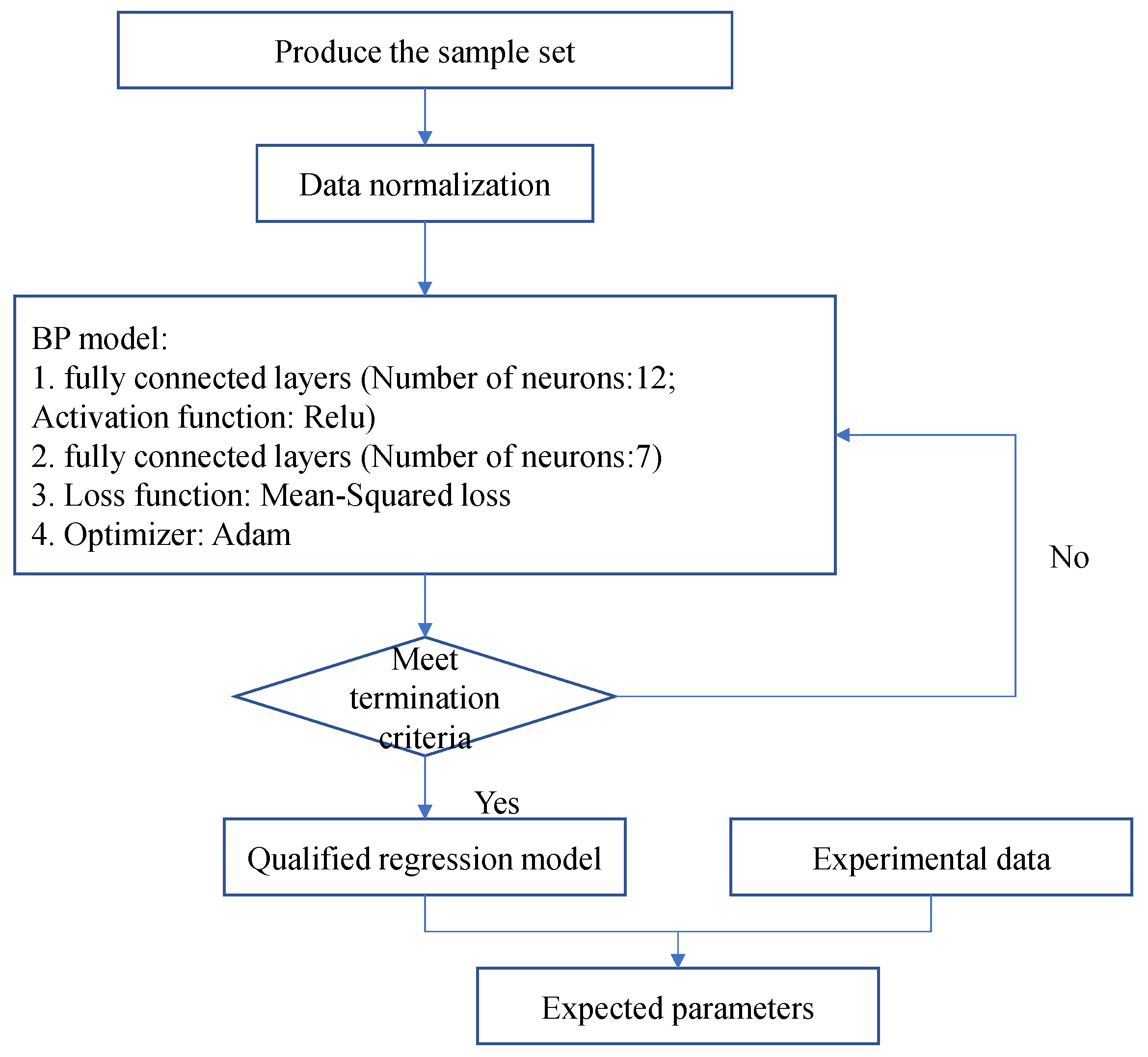
According to the deduction of the constitutive law of each element, the posture of the loading curve is dominated by k11, k12, k2, a, and b; the posture of the unloading curve is dominated by k13’ and b13’; and the massing effect and ratcheting effect are primarily controlled by d and k3. Among these parameters, k13’ and b13’ are relatively independent, particularly for the residual strain. Therefore, the values of k13’ and b13’ are set as shown in Table 4, and the other seven parameters are the objects to be determined by the neural network. In this study, the maximum strain and residual strain in every cycle are considered as inputs with a total of 17 features, and the 7 variable parameters are considered as outputs. The regression procedure is specified as follows, and the corresponding flow is shown in Figure 15.
(a)
Based on the reference values, three different values of each parameter are designated as the labels of the sample set (Table 7). The combination of different parameters results in a total of 2187 samples, of which 90 percent are used for training, and 10 percent are used for validation. By substituting these parameters into the algorithm of the constitutive model, the corresponding strain values can be derived as the features of the sample set.
(b)
Considering an order-of-magnitude difference between each parameter, the Min-Max normalization is used for data preprocessing.
(c)
Constructing a regression model using the BP neural network, which contains one input layer with 17 neurons, one hidden layer with 12 neurons, and one output layer with 7 neurons. The ReLU activation function is used in the hidden layer so as to simulate the nonlinear relation between the input and output, and the Adam optimizer is used to improve the quality of backpropagation. After each iteration, the training loss and validation loss are recorded and saved.
(d)
Setting termination criteria in terms of loss value (magnitude of loss< 0.1 and the change of loss <0.005). If the criteria are satisfied, we can conduct the calibration by introducing the experimental strain data into the qualified regression model. If not, a new iteration begins.

4.2. Results

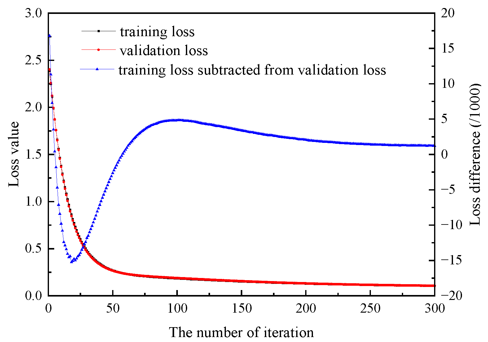
The effect of regression is measured by mean-squared loss between the predicted labels and sample labels, whose values of training loss and validation loss in each iteration are shown in Figure 16. It can be seen that the evolution curves of training loss and validation loss are very close. In order to display the difference between them, the curve of training loss subtracted from validation loss is also added. The first 100 iterations achieved good performances that approached the limit in later iterations with the gradual convergence of the solution. In addition, the decreasing trend of the loss value indicates that the predicted parameters become increasingly credible; the final expected value of each parameter is shown in Table 8.
Applying the determined parameters to the algorithm (Figure 6) with Equations (5), (8), (12), (13), and (15), the simulated stress–strain curves under different conditions can be derived, and comparisons with the experimental curves are shown in Figure 17, from which reasonable accordance can be observed. Moreover, the strains at the peak and residual points in each cycle are extracted, and comparisons between the simulated results and experimental results are displayed in Figure 18. The maximum differences for different conditions are 18%, 6%, and 13%, respectively, which shows a good agreement. In addition, the massing effect and ratcheting effect can be simulated well, which proves that the proposed constitutive model can effectively describe the mechanical behavior under cyclic loading. Thus, the reliability is validated.

5. Conclusions

Aiming at the limitations of the existing constitutive model in terms of synthetically reflecting the massing effect, ratcheting effect, and Felicity effect of rock under cyclic loading and unloading, this study developed a new model that can describe the cyclic mechanical behavior of hard rock sufficiently and agree with physical understanding. In addition, the parameters of the model are calibrated using the neural network. The primary conclusions of this study are as follows:
(1)
By combining the uniaxial cyclic compression on the granite sample with AE monitoring, it is found that the loading process exhibits both elastic deformation and plastic deformation regardless of the stage that the rock sample is currently in. In addition, the mechanical behaviors during the unloading process and reloading process before the Kaiser point are primarily elastic deformation, accompanied by the obstruction of friction between inner cracks. When the loading exceeds the Kaiser point, the plastic strain will continue to develop.
(2)
The cyclic behavior of granite is simulated by a proposed comprehensive body that consists of an elastic element Ee, a plastic element Ep, and a friction element Ef, in which Ef is connected in parallel with the serial combination of Ee and Ep. The opposite effect of Ef during the unloading process and reloading process produces the massing effect, and the plastic deformation during reloading is prompted prior to the historical maximum stress, which brings about the ratcheting effect and Felicity effect.
(3)
In terms of hard rock such as granite, the elasticity reflected by the tangential modulus is affected by elastic strain and plastic strain. The elastic strain dominates the variation process of elasticity, while plastic strain determines the lower limit. Specifically, the tangential modulus of the elastic element exhibits a linear positive correlation with elastic strain, while the lower limit decreases linearly with the plastic strain. In addition, the plastic deformation grows from fast to slow throughout the deformation process, which can be simulated by the Logistic equation.
(4)
The proposed model and corresponding parameters are validated by comparison with the experimental stress–strain curves under three different conditions, and the strain (peak strain and residual strain in each cycle) differences between simulated results and experimental results for different conditions are basically less than 18%, 6%, and 13%, respectively, which strengthens the reliability. In addition, it is worth noting that even though the proposed model holds for the uniaxial compression case, the modeling flow could be extended to other applications, such as triaxial compression, and this paper provides a reference for future research on the cyclic behavior of other materials.

Author Contributions

H.F.: Conceptualization, methodology, writing—review and editing, project administration, funding acquisition. J.L.: software, validation, formal analysis, writing—original draft preparation, writing—review and editing, visualization. G.L.: investigation, resources, data curation, supervision. D.L.: validation, formal analysis, supervision. All authors have read and agreed to the published version of the manuscript.

Funding

This research was supported by the National Natural Science Foundation of China (No.51978668) and China Railway First Survey and Design Institute Group Co., Ltd. through Sichuan-Tibet railway tunnel program (No.19-15-2).

Institutional Review Board Statement

Not applicable.

Informed Consent Statement

Not applicable.

Data Availability Statement

Not applicable.

Acknowledgments

The authors appreciate the editors and anonymous reviewers for their valuable comments and suggestions.

Conflicts of Interest

The authors declare no conflict of interest.

References

  1. Bagde, M.; Petroš, V. Fatigue properties of intact sandstone samples subjected to dynamic uniaxial cyclical loading. Int. J. Rock Mech. Min. Sci. 2005, 42, 237–250. [Google Scholar] [CrossRef]
  2. Chen, H.; Cong, T.N.; Yang, W.; Tan, C.; Li, Y.; Ding, Y. Progress in electrical energy storage system: A critical review. Prog. Nat. Sci. 2009, 19, 291–312. [Google Scholar] [CrossRef]
  3. Li, C.; Liu, N.; Liu, W.; Feng, R. Study on Characteristics of Energy Storage and Acoustic Emission of Rock under Different Moisture Content. Sustainability 2021, 13, 1041. [Google Scholar] [CrossRef]
  4. Gong, F.-Q.; Wu, C.; Luo, S.; Yan, J.-Y. Load–unload response ratio characteristics of rock materials and their application in prediction of rockburst proneness. Bull. Eng. Geol. Environ. 2019, 78, 5445–5466. [Google Scholar] [CrossRef]
  5. Zhu, X.; Li, Y.; Wang, C.; Sun, X.; Liu, Z. Deformation Failure Characteristics and Loading Rate Effect of Sandstone Under Uniaxial Cyclic Loading and Unloading. Geotech. Geol. Eng. 2019, 37, 1147–1154. [Google Scholar] [CrossRef]
  6. Imre, B.; Räbsamen, S.; Springman, S.M. A coefficient of restitution of rock materials. Comput. Geosci. 2008, 34, 339–350. [Google Scholar] [CrossRef]
  7. Chen, Y.P.; Wang, S.J.; Wang, E.Z. Quantitative Study on Stress-strain Hysteretic Behaviors in Rocks. Chin. J. Rock Mech. Eng. 2007, 26, 4066–4073. [Google Scholar]
  8. Wen, T.; Tang, H.; Wang, Y.; Ma, J.; Fan, Z. Mechanical Characteristics and Energy Evolution Laws for Red Bed Rock of Badong Formation under Different Stress Paths. Adv. Civ. Eng. 2019, 2019, 8529329. [Google Scholar] [CrossRef]
  9. Xi, D.Y.; Chen, Y.P.; Tao, Y.Z.; Liu, Y.C. Nonlinear Elastic Hysteric Characteristics of Rocks. Chin. J. Rock Mech. Eng. 2006, 25, 1086–1093. [Google Scholar]
  10. Meng, Q.; Zhang, M.; Han, L.; Pu, H.; Nie, T. Effects of Acoustic Emission and Energy Evolution of Rock Specimens Under the Uniaxial Cyclic Loading and Unloading Compression. Rock Mech. Rock Eng. 2016, 49, 3873–3886. [Google Scholar] [CrossRef]
  11. Meng, Q.; Zhang, M.; Han, L.; Pu, H.; Chen, Y. Acoustic Emission Characteristics of Red Sandstone Specimens Under Uniaxial Cyclic Loading and Unloading Compression. Rock Mech. Rock Eng. 2018, 51, 969–988. [Google Scholar] [CrossRef]
  12. Wang, T.; Wang, C.; Xue, F.; Wang, L.; Teshome, B.H.; Xue, M. Acoustic Emission Characteristics and Energy Evolution of Red Sandstone Samples under Cyclic Loading and Unloading. Shock Vib. 2021, 2021, 8849137. [Google Scholar] [CrossRef]
  13. Li, Y.; Zhao, T.; Li, Y.; Chen, Y. A five-parameter constitutive model for hysteresis shearing and energy dissipation of rock joints. Int. J. Min. Sci. Technol. 2022, in press. [CrossRef]
  14. McCall, K.R.; Guyer, R.A. Equation of state and wave propagation in hysteretic nonlinear elastic materials. Geophys. Res. 1994, 99, 23887–23897. [Google Scholar] [CrossRef]
  15. Scalerandi, M.; Gliozzi, A.; Idjimarene, S. Power laws behavior in multi-state elastic models with different constraints in the statistical distribution of elements. Commun. Nonlinear Sci. Numer. Simul. 2014, 19, 3628–3641. [Google Scholar] [CrossRef]
  16. Chen, X.; Huang, Y.; Chen, C.; Lu, J.; Fan, X. Experimental study and analytical modeling on hysteresis behavior of plain concrete in uniaxial cyclic tension. Int. J. Fatigue 2017, 96, 261–269. [Google Scholar] [CrossRef]
  17. Wang, X.; Song, L.; Gao, X.; Chang, X. Effect of loading rate on the nonlinear elastic response of concrete. Eur. J. Environ. Civ. Eng. 2021, 25, 909–923. [Google Scholar] [CrossRef]
  18. Hua, D.; Jiang, Q. Three-Dimensional Modeling of Hysteresis in Rocks. J. Geophys. Res. Solid Earth 2022, 127, e2021JB023230. [Google Scholar] [CrossRef]
  19. Hashiguchi, K. Generalized plastic flow rule. Int. J. Plast. 2005, 21, 321–351. [Google Scholar] [CrossRef]
  20. Kong, L.; Zheng, Y.R.; Yao, Y.P. Subloading surface cyclic plastic model for soil based on Generalized plasticity (I): Theory and model. Rock Soil Mech. 2003, 24, 141–145. [Google Scholar] [CrossRef]
  21. Kong, L.; Zheng, Y.R.; Yao, Y.P. Subloading surface cyclic plastic model for soil based on Generalized plasticity (II): Constitutive equation and identification. Rock Soil Mech. 2003, 24, 349–354. [Google Scholar] [CrossRef]
  22. Zhou, Y.Q.; Sheng, Q.; Zhu, Z.Q.; Fu, X.D. Subloading surface model for rock based on modified Drucker-Prager criterion. Rock Soil Mech. 2017, 38, 400–418. [Google Scholar] [CrossRef]
  23. Zhou, Y.; Sheng, Q.; Li, N.; Fu, X.; Zhang, Z.; Gao, L. A constitutive model for rock materials subjected to triaxial cyclic compression. Mech. Mater. 2020, 144, 103341. [Google Scholar] [CrossRef]
  24. Valanis, K.C.; Fan, J. A numerical algorithm for endochronic plasticity and comparison with experiment. Comput. Struct. 1984, 19, 717–724. [Google Scholar] [CrossRef] [Green Version]
  25. Cerfontaine, B.; Charlier, R.; Collin, F.; Taiebat, M. Validation of a New Elastoplastic Constitutive Model Dedicated to the Cyclic Behaviour of Brittle Rock Materials. Rock Mech. Rock Eng. 2017, 50, 2677–2694. [Google Scholar] [CrossRef] [Green Version]
  26. Liu, D.; He, M.; Cai, M. A damage model for modeling the complete stress–strain relations of brittle rocks under uniaxial compression. Int. J. Damage Mech. 2018, 27, 1000–1019. [Google Scholar] [CrossRef]
  27. Wu, Y.L.; Chen, J.; Zeng, S.M. The Acoustic Emission Technique Research on Dynamic Damage Characteristics of the Coal Rock. Procedia Eng. 2011, 26, 1076–1082. [Google Scholar] [CrossRef] [Green Version]
  28. Kong, X.; Wang, E.; He, X.; Zhao, E.; Zhao, C. Mechanical characteristics and dynamic damage evolution mechanism of coal samples in compressive loading experiments. Eng. Fract. Mech. 2019, 210, 160–169. [Google Scholar] [CrossRef]
  29. Xiao, J.-Q.; Ding, D.-X.; Jiang, F.-L.; Xu, G. Fatigue damage variable and evolution of rock subjected to cyclic loading. Int. J. Rock Mech. Min. Sci. 2010, 47, 461–468. [Google Scholar] [CrossRef]
  30. Liu, E.; He, S. Effects of cyclic dynamic loading on the mechanical properties of intact rock samples under confining pressure conditions. Eng. Geol. 2012, 125, 81–91. [Google Scholar] [CrossRef]
  31. Wang, Z.; Li, S.; Qiao, L.; Zhao, J. Fatigue Behavior of Granite Subjected to Cyclic Loading Under Triaxial Compression Condition. Rock Mech. Rock Eng. 2013, 46, 1603–1615. [Google Scholar] [CrossRef]
  32. Chen, Y.; Zuo, J.; Guo, B.; Guo, W. Effect of cyclic loading on mechanical and ultrasonic properties of granite from Maluanshan Tunnel. Bull. Eng. Geol. Environ. 2020, 79, 299–311. [Google Scholar] [CrossRef]
  33. Li, X.W.; Yao, Z.S.; Huang, X.W.; Liu, Z.X.; Zhao, X.; Mu, K.H. Investigation of deformation and failure characteristics and energy evolution of sandstone under cyclic loading and unloading. Rock Soil Mech. 2021, 42, 1693–1704. [Google Scholar]
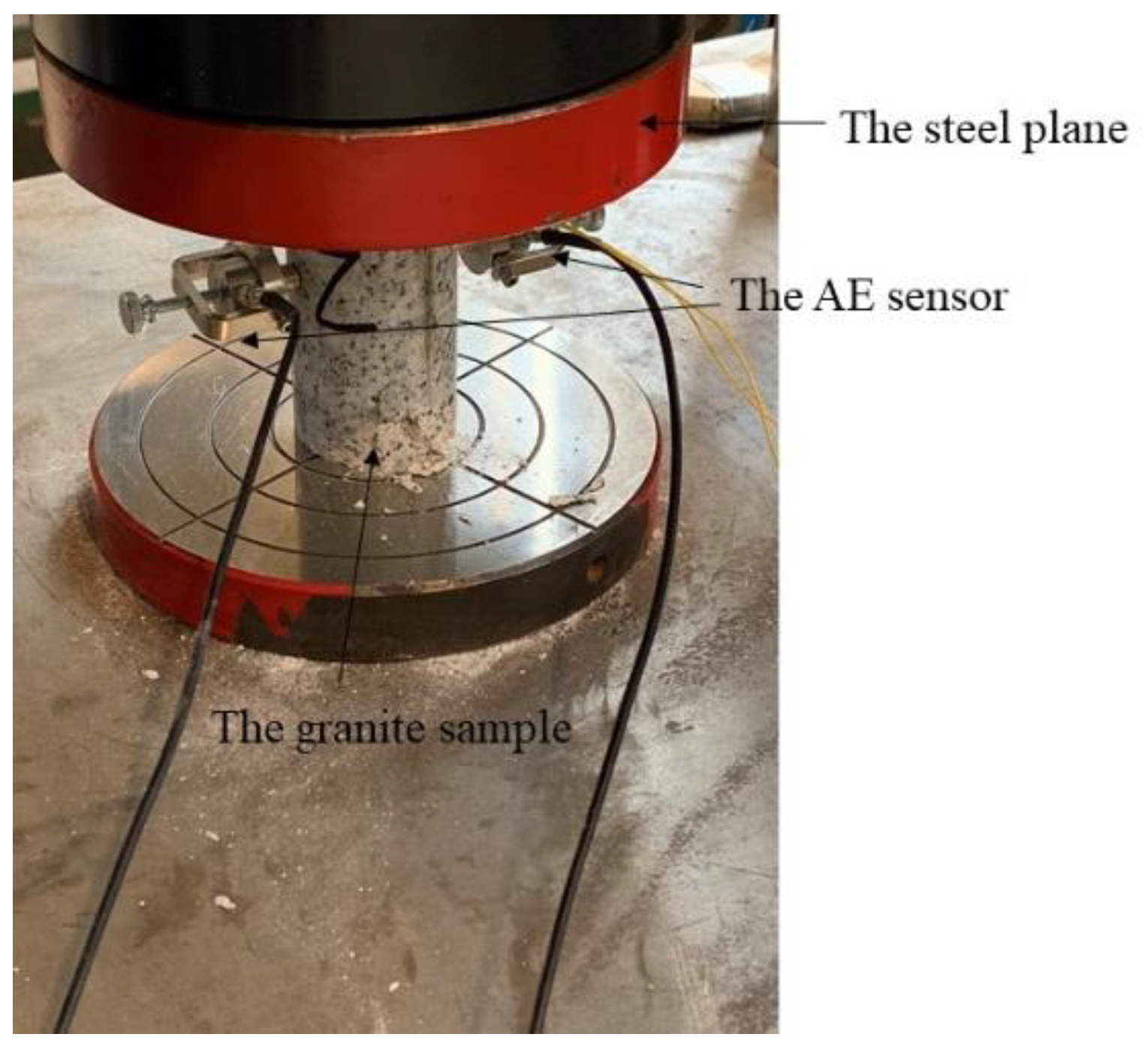
Figure 1. Experimental setup.
Sustainability 14 10412 g001
Figure 2. Stress–strain curves of the rock samples under uniaxial cyclic loading and unloading.
Sustainability 14 10412 g002
Figure 3. Variations in stress and AE hits with time (the blue horizontal dashed lines denote the peak stress in each cycle, while the vertical dashed lines denote the moment when AE hits increase abruptly). (a) vl = 0.6 mm/min. (b) vl = 0.9 mm/min. (c) vl = 1.2 mm/min.
Sustainability 14 10412 g003
Figure 4. Schematic loading and unloading in two cycles.
Sustainability 14 10412 g004
Figure 5. Comprehensive body for describing the cyclic behavior.
Sustainability 14 10412 g005
Figure 6. Algorithm for modeling cyclic behavior.
Sustainability 14 10412 g006
Figure 7. Elastic strain of the peak point in each cycle and the corresponding fitting relationship between εe and σ.
Sustainability 14 10412 g007
Figure 8. εe-σ relationship of the loading process throughout the test and the stress–strain curve of the unloading process in each cycle. (a) vl = 0.6 mm/min. (b) vl = 0.9 mm/min. (c) vl = 1.2 mm/min.
Sustainability 14 10412 g008
Figure 9. Tangential modulus k13 and residual strain εr at the endpoint of the unloading path in each cycle and the corresponding fitting relationship.
Sustainability 14 10412 g009
Figure 10. Gradient variation of the unloading path for each cycle and the corresponding fitting relationship between the gradient and ε. (a) vl = 0.6 mm/min. (b) vl = 0.9 mm/min. (c) vl = 1.2 mm/min.
Sustainability 14 10412 g010
Figure 11. Variation of plastic strain increment with the peak stress.
Sustainability 14 10412 g011
Figure 12. Plastic strain of the peak point in each cycle and the corresponding fitting relationship between εp and σ.
Sustainability 14 10412 g012
Figure 13. Schematic stress–strain curve without the ratcheting effect and curve with the ratcheting effect. (a) Defective stress–strain curve. (b) Real stress–strain curve.
Sustainability 14 10412 g013
Figure 14. Variation the yield surface during the loading and unloading process.
Sustainability 14 10412 g014
Figure 15. Regression flow of the parameters to be determined.
Sustainability 14 10412 g015
Figure 16. Variation of loss with the increased iteration.
Sustainability 14 10412 g016
Figure 17. Comparison of the stress–strain curve under variable amplitude loading between the simulated results and experimental results. (a) vl = 0.6 mm/min. (b) vl = 0.9 mm/min. (c) vl = 1.2 mm/min.
Sustainability 14 10412 g017
Figure 18. Comparison of peak strain and residual strain in each cycle between the simulated and experimental results. (a) vl = 0.6 mm/min. (b) vl = 0.9 mm/min. (c) vl = 1.2 mm/min.
Sustainability 14 10412 g018
Table 1. Mineralogical composition of the rock samples.
Quartz (%)K-Feldspar (%)Plagioclase (%)Biotite (%)Others (%)
35.1128.2130.645.450.59
Table 2. Physical and mechanical properties of rock samples.
Water Content (%)Density (g/cm3)Dry Density (g/cm3)Velocity of Longitudinal Waves (m/s)Schmidt HardnessUCS (MPa)Uniaxial Tensile Strength (MPa)
0.092.72.6307769150.04.8
Table 3. Parameters for fitting f(εe) during loading.
k11k12R2
vl = 0.6 mm/min8391.261,075,623.840.9977
vl = 0.9 mm/min9152.611,270,575.230.9974
vl = 1.2 mm/min13,657.93452,678.390.9986
Table 4. Parameters for fitting the relationship between k13 and εp.
k13b13R
vl = 0.6 mm/min−4,487,92012,859.92−0.8751
vl = 0.9 mm/min−3,298,22010,145.63−0.9333
vl = 1.2 mm/min−5,555,45017,057.99−0.9681
Table 5. Parameters for fitting g(εp).
k2abR2
vl = 0.6 mm/min183.345.022337.400.9967
vl = 0.9 mm/min192.884.872401.320.9944
vl = 1.2 mm/min702.447.162896.710.9244
Table 6. Felicity ratio RF for each cycle.
Cycle 2Cycle 3Cycle 4Cycle 5Cycle 6Cycle 7Cycle 8Cycle 9
vl = 0.6 mm/min1.160.980.970.950.930.910.890.87
vl = 0.9 mm/min1.130.980.970.970.960.950.940.91
vl = 1.2 mm/min1.080.980.980.970.970.950.950.93
Table 7. Parameters for producing the sample set.
k11k12k2abdk3
vl = 0.6 mm/min7000, 8000, 90009 × 105, 1.0 × 10⁶, 1.1 × 106150, 200, 2503, 5, 72000, 3000, 40000.0001, 0.0005, 0.000910, 20, 30
vl = 0.9 mm/min7000, 8000, 90001.1 × 106, 1.2 × 10⁶, 1.3 × 106150, 200, 2503, 5, 72000, 3000, 40000.0001, 0.0005, 0.000910, 20, 30
vl = 1.2 mm/min12,000, 13,000, 14,0004 × 10⁵, 5 × 10⁵, 6 × 105650, 700, 7505, 7, 92000, 3000, 40000.0001, 0.0005, 0.000910, 20, 30
Table 8. Determined value of each parameter used in the proposed constitutive model.
k11k12k2abdk3
vl = 0.6 mm/min72791,039,693164.65.73356.20.0005117.8
vl = 0.9 mm/min85091,142,430241.36.23573.30.0002415.2
vl = 1.2 mm/min12,237569,2637027.233000.0001313.7
Publisher’s Note: MDPI stays neutral with regard to jurisdictional claims in published maps and institutional affiliations.