Influence of Population Agglomeration on Urban Economic Resilience in China

Abstract

Under the background of complex domestic and international environment and the trend of urban population agglomeration, the impact of population agglomeration on urban economic resilience is worthy of attention. This paper uses a sample of 284 cities in China to empirically analyze the impact of population agglomeration on urban economic resilience in the context of the 2008 international financial crisis with the help of spatial econometric models. The results are as follows. First, population agglomeration can enhance the city’s resistance to the economic crisis, is more conducive to improving the city’s economic recovery and adjustment ability, and has a positive spatial spillover effect on surrounding cities. Moreover, population agglomeration enhances the economic resilience of urban secondary and tertiary industries. Secondly, in the population agglomeration context, the situation of the labor force structure affects the resilience of the urban economy. In terms of the labor force’s age structure, the agglomeration of prime-age labor is more conducive to improving urban economic resilience than youth and old labor. In terms of labor quality structure, homogeneous human capital agglomeration enhances cities’ resistance to economic crisis, while heterogeneous human capital agglomeration enhances cities’ ability to recover and adjust their economy.

1. Introduction

From the perspective of global economic development, population agglomeration is a common state of economic and social development in all countries in the world, and the trend of population agglomeration to economically developed regions is very significant. As the main gathering place of various human activities, cities are the main gathering place of human activities and are important carriers of national economic and social development, and also the main place of population gathering. With the further development of the economy, China’s urbanization level is increasing rapidly. The seventh census report shows that, in 2020, the country’s urban resident population was 902 million, with an urbanization rate of 63.89 percent and an increase of 14.21 percentage points over 2010. Driven by increasingly lax settlement policies, population mobility has become easy and urban population agglomeration pronounced. Population agglomeration has provided a sufficient labor force for China’s urbanization and industrialization and has made great contributions to China’s economic development [1]. However, in the globalization context, the construction of global production networks is gradually improving. As a link between regional and global economic networks, urban development is considerably vulnerable to global financial crises, volatile foreign trade environment, and industrial restructuring. In this context, urban economic resilience is emerging as a cutting-edge topic in regional research, which focuses on the resilience of regional economic systems to crises by transforming their economic structures and functions amidst external shocks and disruptions, and on their ability to absorb, understand, and resolve crises for regrowth [2,3,4]. With the further development of China’s economy, the trend of population agglomeration in cities is difficult to change in a short period, so the impact of population agglomeration on urban economic resilience should be studied. However, less attention has been paid to the impact of China’s population agglomeration on urban economic resilience in existing studies. Therefore, this paper takes the main cities of China as a research object and carries on the empirical analysis of the population agglomeration under the 2008 financial crisis and labor force structure to urban economic resilience influence, thereby providing theoretical support for population agglomeration strategies that enhance urban economic resilience.

The marginal contributions of this paper are: first, from a research perspective, the economic resilience perspective is introduced into the research on population agglomeration and economic development, and the impact of population agglomeration on urban economic resilience is systematically analyzed from both theoretical and empirical levels. In terms of mechanism analysis, it specifically analyzes the impact of labor age and quality structure on urban economic resilience under the background of population agglomeration, enriching theoretical and practical research on the relationship between population agglomeration and economic resilience. Third, in terms of measurement methods, considering the spatial correlation of research variables, the spatial econometric model is used to analyze the relationship between the two and to test whether the impact of population agglomeration on urban economic resilience has spillover effects.

The remainder of this paper is structured as follows: the first part uses the existing theory as the basis in proposing the hypothesis on the impact of population agglomeration on urban economic resilience. The second part establishes the model. The third part describes the temporal and spatial characteristics of economic resilience and population agglomeration in major Chinese cities after the 2008 financial crisis. The fourth part presents an empirical study. Lastly, the fifth concludes this research.

2. Theory and Hypothesis

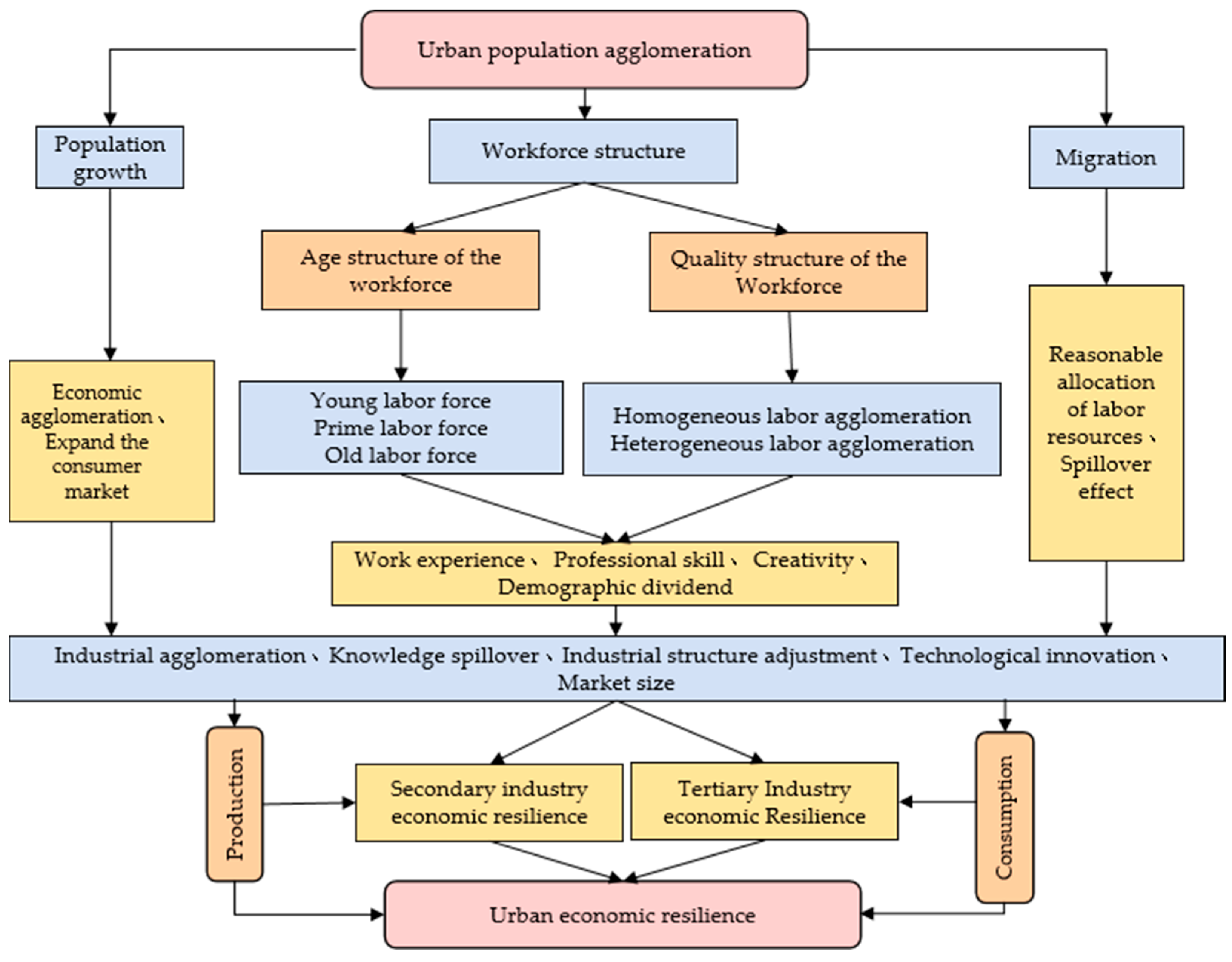
2.1. Impact of Population Agglomeration on Urban Economic Resilience

Population agglomeration is both a resulting state and a process. Specifically, population agglomeration refers to a state of uneven distribution of population within a country or a region. At the same time, due to the slow change in the current natural population growth rate, mechanical population growth has become the main factor in regional population changes; therefore, the dynamic meaning of population Agglomeration is equivalent to population migration. The theory of population migration shows that population agglomeration to cities is a general law of economic development. For example, Lewis’ research points out that a dual economy prevails in developing countries. The urban industrial sector has higher wages than the agricultural sector, and there is a large amount of surplus labor in the traditional agricultural sector. In pursuit of greater returns, it will shift to the urban industrial sector [5]. The push-pull theory of population migration shows that there is a “pull” in cities that is conducive to the improvement and development of individual life [6,7,8]. Population is the main body of social and economic activities and the unity of productive forces and consumption. Undoubtedly, population agglomeration is crucial to urban economic development. That is, population agglomeration will also affect the resilience of cities after suffering from external economic crises. From the perspective of evolutionary economic geography, economic resilience includes regional resistance to shocks, vulnerability to performance, and the ability to recover from crises and adjust and upgrade [3,4,9]. Accordingly, this paper defines the resilience of the urban economy from two aspects: resilience of the fragile resistance period and resilience of the recovery adjustment period. In particular, urban economic resilience during fragile resilience refers to the ability of cities to withstand and absorb shocks during economic crises. By contrast, urban economic resilience during the recovery period refers to the ability of cities to recover from shocks, integrate internal resources, adjust their structures, and adapt to a new external environment. According to the above theory, this part focuses on the analysis of the impact mechanism of population agglomeration on urban economic resilience (Figure 1), and presents assumptions.

Existing research has indicated that population agglomeration directly manifests itself in the expansion of urban population size, which, as a proxy variable for agglomeration economy, will affect cities’ resilience to crises and recovery from economic shocks [10]. In the fragile resistance period when an economic crisis occurs, cities with high concentrations of the population tend to develop an agglomeration economy, thereby leading to a high economic development foundation and rapid economic growth. If the crises suffered by cities are within the tolerable range, then the concentration of labor force and human capital in the context of urban population agglomeration can further protect cities from the impact of economic crises. Capello shows that cities or densely populated areas show significant resilience performance [11]. Xi Huang shows that metropolitan areas with a larger immigrant population tended to better preserve their growth paths during the Great Recession and to experience greater levels of employment and per capita income growth following the recession [12]. After economic crises, cities will enter a long period of recovery and adjustment. At present, the agglomeration of the urban population mainly promotes the recovery and development of the urban economy by increasing labor force supply, promoting population structure rejuvenation, improving labor force quality, and increasing effective demand. First, population agglomeration increases the supply of urban labor, resulting in a “labor pool effect”, the agglomeration of multi-skilled labor provides talent support for cities to develop emerging technology industries, promoting the adjustment and upgrading of the urban economy and improves the resilience of the urban economy. Secondly, population agglomeration promotes the rejuvenation of the urban population structure and brings demographic dividends to economic development. Thirdly, during the fragile resistance period, the surplus labor force generated by layoffs by enterprises has been re-employed one after another, completed labor skills training, and re-invested in new production activities. In this part of labor, through further training, the quality of employees has been significantly improved and has become an important human capital basis for the development of emerging enterprises [13]. Lastly, enterprises’ economic recovery has stabilized labor income. Moreover, the agglomeration of the urban population has increased consumer demand, expanded domestic demand, relatively alleviated the adverse impact of the deterioration of foreign trade, and further increased the pace of urban economic recovery. In addition, the trend of population agglomeration leads to significant inter-city population mobility, which is conducive to the rational allocation of labor resources, and the labor force with high skills tends to have high mobility [14]. Cross-regional population mobility can effectively promote the formation and diffusion of new knowledge and new technologies and enhance urban innovation capabilities [15] to provide favorable technical support for the economic development of impacted and surrounding cities and improve the urban economic resilience [16]. Consequently, the impact of population agglomeration on urban economic resilience has a certain positive spillover effect. Therefore, this paper proposes the following hypothesis:

Hypothesis (H1).

Population agglomeration has a positive impact on urban economic resilience, with a positive spillover effect.

Secondary industry is the cornerstone of urban economic development. Given the further improvement of urbanization, the prosperity of the tertiary industry is also an important feature of modern urban economic development. Therefore, the secondary and tertiary industries are critical to urban economic development. These industries’ ability to withstand and recover from international financial crises determines the level of economic resilience of cities. Population agglomeration is closely related to the development of the two industries, but its impact mechanism on their economic resilience is different. In particular, population agglomeration mainly affects the economic resilience of the secondary industry by restricting production development. Population agglomeration provides sufficient labor and technical talents for the secondary industry to withstand shocks and recover and adjust, and significantly improves the economic resilience of the urban secondary industry. The impact of population agglomeration on the economic resilience of the tertiary industry focuses on the perspective of consumption. That is, cities with high population agglomeration in the fragile resistance period can rely on high consumer demand to maintain the steady development of the urban tertiary industry, thereby enhancing the resistance of the tertiary industry to economic crises. In the recovery and adjustment period, population agglomeration in cities will promote the expansion of consumer demand and upgrading of consumption structure, which is conducive to the recovery and adjustment of the tertiary industry economy, thereby enhancing the economic resilience of the tertiary industry. Therefore, this paper extends H1 as follows:

Hypothesis (H1.1).

Population agglomeration can improve the economic resilience of urban secondary and tertiary industries.

2.2. Changes in Labor Structure under Population Agglomeration Affect Urban Economic Resilience

Population migration is a human capital investment behavior, which is a reflection of the population on spatial differences in labor market opportunities and costs [17,18]. As a result of population migration, population agglomeration has a direct impact on the population structure of cities, with the age labor force structure being the most affected. The labor force, as the main body of the entire social production behavior, has a direct influence on the development of the urban economy. The change of labor force structure caused by population agglomeration will inevitably affect the resilience of the urban economy. For a long time, academia has focused on the impact of labor force age structure and quality on economic development. To further analyze the impact mechanism of population agglomeration on urban economic resilience, this paper also analyzes the labor force age structure and quality. First of all, from the perspective of the age structure of the working population, the 40–54-year-old labor force, as the main force in the labor market, is an important support for urban economic development, and it is well documented that experience and the accumulation of work-related knowledge imply a peak in life-cycle productivity around age 40 to 54 years [19,20], with rich work experience and good physical strength, this type of labor gathering can ensure the stable development of the city’s economy, enhance the city’s ability to resist economic crises, and provide excellent labor support for the recovery and adjustment of the city’s economy. However, compared with the prime-age labor force, part of the 15–40-year-old youth labor force is still in the education stage, the labor force participation rate is low, and due to the relatively short working hours, the work experience is obviously relatively insufficient, and the mobility of the youth age labor force is stronger than that of the prime-age labor force, so its resilience to the economic crisis is weaker than that of the prime-age labor force. The 54–65-year-old labor force is physically weaker than the prime-age and young labor force, and generally has a weak ability to accept emerging technologies [21], and the labor force participation rate is relatively low; therefore, its effect on urban economic resilience is also smaller than that of prime-age labor, and it may even have an adverse impact on urban economic recovery and adjustment. Therefore, this paper proposes the following hypothesis:

Hypothesis (H2).

Compared with the youth labor force and the old labor force, the agglomeration of the prime-age labor force has the greatest significance for urban economic resilience.

The human capital variable is a commonly used variable to reflect the quality level of the labor force. According to whether or not human capital has the attribute of increasing returns, the labor force is divided into homogenous and heterogeneous human capital [22]. The impact of the two types of the labor force on urban economic resilience is different. In general, the labor skills of a homogenous labor force are relatively simple but highly specialized. Its agglomeration can provide numerous professional and technical personnel for urban economic development and relatively improve the ability of cities to withstand economic crises. However, the long-term agglomeration of the single-skill labor force tends to cause path dependence, confines related enterprises to the original development mode, and results in difficulty meeting the needs of urban economic adjustment and upgrading. By contrast, heterogeneous human capital generally has diversified labor skills, which enables this type of labor to have a wider range of employment options, and it is easier to achieve re-employment if unemployed under the impact of the economic crisis. Reducing urban unemployment enables cities to have good resilience performance [23]. Moreover, this type of population agglomeration is often accompanied by technological progress [24]. This type of labor force enables cities to maximize existing technological resources to find new opportunities, new industries to replace sunset industries, high value-added industries to replace low value-added industries, break pathways of dependence and promote the adjustment and upgrading of urban industrial structures [25], and improve urban economic resilience. Agglomeration of heterogeneous human capital is also conducive to promoting the upgrade of residents’ consumption [26,27], generating new consumption demands, prompting enterprises to innovate in production, and injecting new vitality into economic development. Therefore, long-term heterogeneous human capital agglomeration is crucial to the improvement of urban economic resilience. Accordingly, the following hypothesis is formulated:

Hypothesis (H3).

Homogeneous human capital agglomeration enhances cities’ resistance to economic crises, while heterogeneous human capital agglomeration enhances cities’ ability to recover and adjust their economy.

3. Methods and Variables

3.1. Model Settings

Spatial econometric models take into account the non-independence of adjacent regions. Spatial econometric models should be used to analyze when the properties of the research object are related spatially. The most commonly used econometric models are Spatial Lag Model (SLM), Spatial Error Model (SEM), and Spatial Durbin Model (SDM). In order to fully consider the effects of spatial factors, a spatial measurement model of the effects of urban population agglomeration on economic resilience was established. The model formula is as follows:

$$\begin{array}{l}Y=\rho WY+\beta X+\theta WX+\mu \\ \mu =\lambda W\mu +\epsilon ,\epsilon \sim N[0,{\sigma }^{2}I]\end{array}$$

(1)

In the Formula (1), Y is the dependent variable, X is the independent variable; the independent variable parameter β represents the influence coefficient of the independent variable on the dependent variable, and ρ is the spatial autocorrelation coefficient, which is used to reflect the influence of the spillover of the explained variables of neighboring cities on the same attributes of the city itself; W is the spatial weight matrix, this study uses the rook weight matrix, that is, the weight of city adjacent is 1, the weight of non-adjacent is 0, WY is the lag term of the dependent variable, θ represents the coefficient of influence of independent variables in surrounding areas on the region; µ and ε represent random errors, and ε follows a positive. When ρ ≠ 0, θ = 0 and λ = 0, it conforms to the spatial lag model (SLM); when ρ = 0, θ = 0 and λ ≠ 0, it conforms to the spatial error model (SEM); ρ ≠ 0, When θ ≠ 0 and λ = 0, it conforms to the spatial Durbin model (SDM).

3.2. Variable Description

3.2.1. Urban Economic Resilience

In the measurement of urban economic resilience, the regional economic resilience measurement method of Martin et al., which has achieved consensus, is adopted [3]. This method expresses the relative resilience of cities in the face of shocks by calculating the sensitivity of economic indicators in various regions during the economic crisis. The formula is:

$$\mathrm{Re}si{s}_i^t=(\Delta Y_i-\Delta E)/\left|\Delta E\right|$$

(2)

In the formula (2): $\mathrm{Re}si{s}_i^T$ represents the relative economic resilience of city i in period T. When $\mathrm{Re}si{s}_i^T$ > 0, the economic operation of city i exceeds the average level of economic operation in the region where it is located, and it is a high-resilience city; when $\mathrm{Re}si{s}_i^T$ < 0, the economic operation of city i. It is lower than the average level of economic operation in the region where it is located, and it is a low-resilience city. ΔY_i is the actual economic operation of city i, calculated by Formula (3); ΔE is the overall economic operation of the region where city i is located, calculated by Formula (4), which represents the expected economic operation of city i:

$$\Delta Y=(Y_i^t-Y_i^{t-k})/Y_i^{t-k}$$

(3)

$$\Delta E=(Y_r^t-Y_r^{t-k})/Y_r^{t-k}$$

(4)

In the formula: $Y_i^t$, $Y_i^{t-k}$ represent the quantitative indicators of city i at time t and t − k. In this study, the “GDP per land” (100 million yuan/km²) of a city is used as a quantitative indicator and brought into Formula (3) to calculate the actual economic development level of city i. In order to ensure data comparability, the GDP of each city from 2009 to 2019 was deflated and brought into the formula based on the GDP value of each city in 2008 to eliminate the impact of price index changes. $Y_r^t$, $Y_r^{t-k}$ are the quantitative indicators at time t and t − k in the area where the research object is located, and are usually calculated based on the national economic development level. However, due to the large differences in the economic development levels of the four major economic sectors in eastern, central, western, and northeastern China, the cities in each economic zone are calculated based on the development level of the four major economic zones. The expected development level of each economic zone is also calculated using the deflated GDP per land (100 million yuan/km²). This study distinguishes two types of economic resilience: (i) fragile resistance period from 2008 to 2010, which is used to represent the fragile and resistance of cities amidst the 2008 global financial crisis; and (ii) recovery and adjustment period from 2010 to 2019, which indicates the ability of cities to recover and adjust economically after the crisis. This division is based on the changing trend of China’s GDP growth rate amidst the 2008 financial crisis (Figure 2). China’s economic growth rate peaked in 2007, and GDP growth decreased sharply after the 2008 financial crisis. In 2010, new features appeared in China’s economic development under the influence of the “Four Trillion Plan”. That is, the economic growth rate was low but moderate. Driven by national macro-control and other policies, most cities in China have adjusted their economic structures and entered a period of recovery and adjustment. Calculate the urban economic resilience and the economic resilience of the secondary and tertiary industries according to the above methods. The data used are from the “China City Statistical Yearbook”.

3.2.2. Urban Population Agglomeration Level

The population agglomeration degree reflects the agglomeration degree of the population of a region relative to the national population, and is the core explanatory variable of this paper. This study calculates the degree of population agglomeration in each city based on the calculation method proposed by Liu Ruiwen [28]. The calculation formula is as follows:

$$JJ{D}_i=\frac{(P_i/P_n)\times 100\%}{(A_i/A_n)\times 100\%}=\frac{P_i/A_i}{P_n/A_n}$$

(5)

In the formula: JJD_i represents the population agglomeration degree of city i. A population agglomeration degree greater than 1 indicates that the population agglomeration level of the city is greater than the national average level, and less than 1 indicates that the urban population agglomeration level is lower than the national average level; P_i is the population of the city i (people); A_i is the area of the city i (km²); P_n is the sum of the urban population in all study areas (person); A_n is the sum of the urban areas in all study areas (km²). According to this method, the urban population agglomeration degree of each city in 2008 and 2010 was calculated. Among them, the population agglomeration degree in 2008 was used as the core explanatory variable of the model related to the fragile resistance period, and the population agglomeration degree in 2010 was used as the core explanatory variable of the recovery adjustment period model. In addition, due to the lack of detailed demographic data in 2008, only the labor force population agglomeration and human capital agglomeration of each age group in 2010 were calculated and used as the common explanatory variables of the two-period model. Specifically, the population of 15–40 years old in each city was used to calculate the concentration of young labor force, the population of 40–54 years old was used to calculate the concentration of prime-age labor force, and the population of 54–65 years old was used to calculate the concentration of elderly labor force. The homogeneous human capital agglomeration degree was measured by the number of the employed population with a degree below a junior college degree (none of school, elementary school, junior high school, high school), and the heterogeneous human capital agglomeration degree was calculated by the number of the population with a junior college degree or above (College, Undergraduate, and Postgraduate). The 2008 urban population agglomeration data in the above variables were calculated based on the urban population data in the 2009 China Urban Statistical Yearbook. The 2010 urban population agglomeration data and the labor force population agglomeration and human capital agglomeration of each age group were calculated based on the urban population data in the 2010 sixth census yearbook of each province.

3.2.3. Control Variables

Based on existing research and the availability of data, this paper selects industrial structure diversity [29,30,31], economic development foundation [3], government policy support [32], level of opening to the outside world [33], market size [3], and science and technology expenditure [34,35] were used as control variables to build the model. First, industrial diversity, as an important indicator of economic resilience, was calculated by the entropy method [36] using industrial population data. The initial economic development level was represented by the GDP data of each city. Government policy support was represented by the fiscal self-sufficiency rate. The level of opening to the outside world was represented by the actual amount of foreign capital used by each city in that year. The total retail and wholesale trade of consumer goods represented the market size of each city. The science and technology expenditure of each city represented the city’s emphasis on scientific and technological development. To narrow the absolute difference between the data, we took the logarithm of the variables of “GDP” and “total retail and wholesale trade of consumer goods”. According to the availability of data and the principle of time proximity, the control variables in the model related to the fragile resistance period (2008–2010) were calculated using the starting year of the period, that is, 2008 data were calculated; the control variables in the model related to the recovery adjustment period (2010–2019) were also calculated using the starting year of the period, that is, 2010 data were calculated. The above control variable data are all from the “China City Statistical Yearbook” (

Table 1. Variable name and data source.

Variable Name	Symbol	Indicator Meaning	Source
Resident population concentration	pop	population agglomeration	“China City Statistical Yearbook” “2010 Provincial Census Data”
Agglomeration of the population aged 15–40	youth	youth labor
Aggregation of population aged 40–54	prime	prime-age labor
Agglomeration of population aged 54–64	elder	older labor
The agglomeration of the population with education below junior college among the employed population	hom	Homogeneous human capital
The agglomeration of the population with college education and above among the employed population	het	Heterogeneous human capital
Science and technology expenditure (100 million yuan)	ste	Innovation level	“China City Statistical Yearbook”
Total retail and wholesale trade of consumer goods (100 million yuan)	cm	market size
GDP (100 million yuan)	lngdp	economic development foundation
Amount of foreign capital actually utilized (USD 10,000)	lnopen	level of opening
financial self-sufficiency rate (%)	fsel	Government policy support
Industrial Diversity	indiv	Industrial Diversity

).

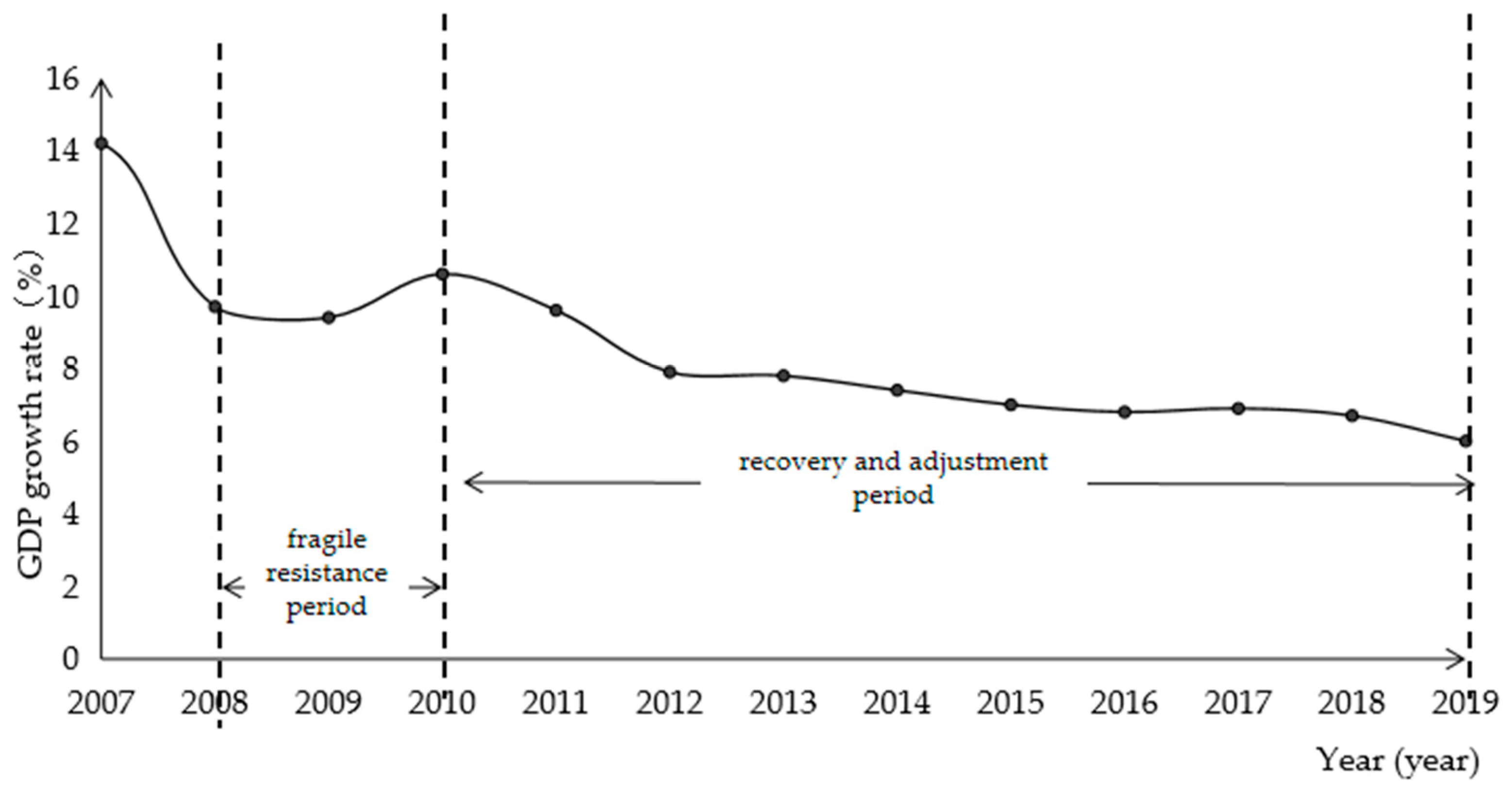
4. Spatial Evolution Characteristics of Urban Economic Resilience and Population Agglomeration

4.1. Spatial Distribution Pattern

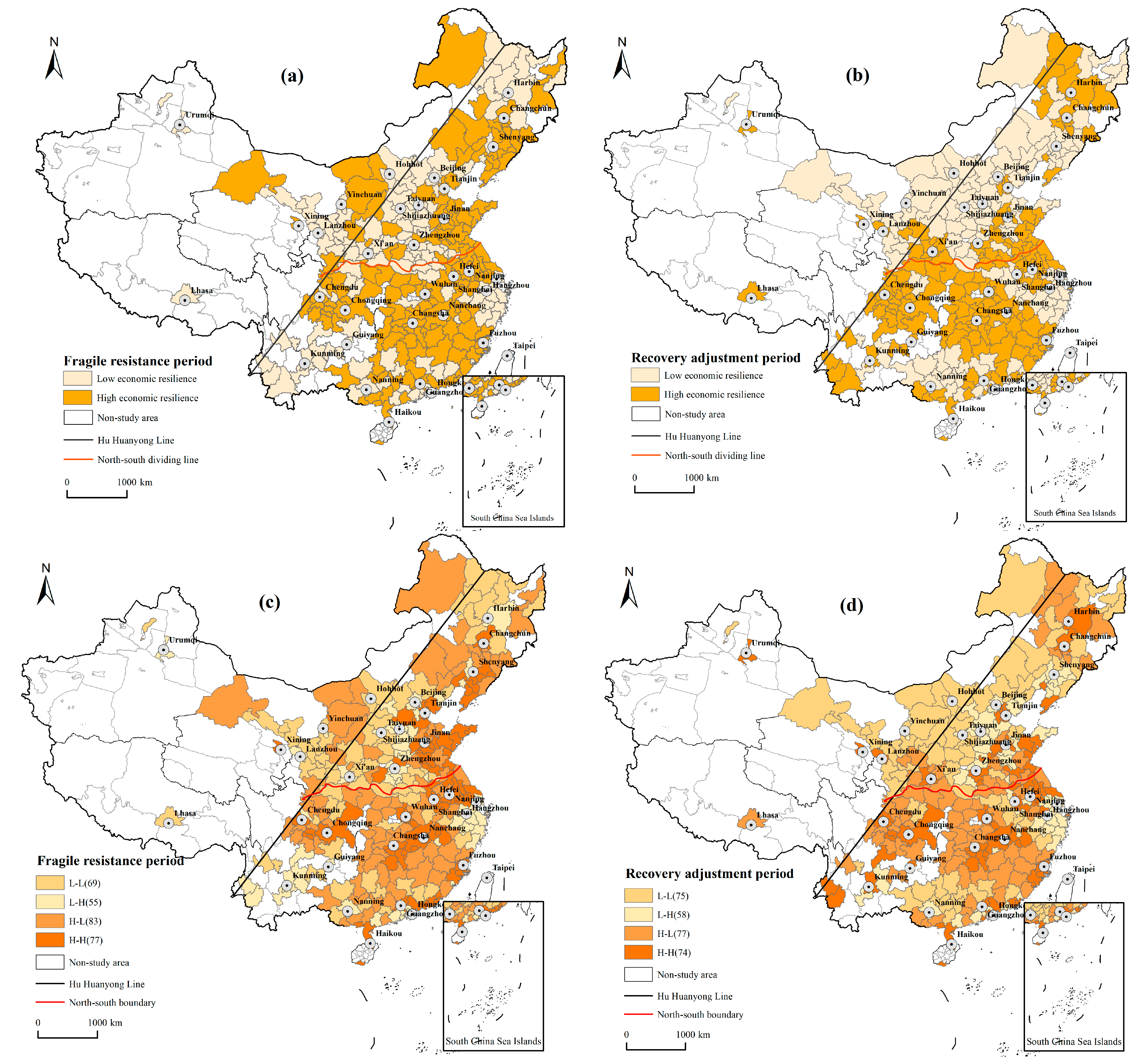
4.1.1. Spatial Distribution Pattern of Urban Economic Resilience

According to Formula (2), the urban economic resilience of 284 Chinese cities in the face of the international financial crisis is measured. According to the calculation results,

Table 2. Number of economically resilient cities in each period.

Period	Low Resilience City		High Resilience City
	Number (Pieces)	Proportion (%)	Number (Pieces)	Proportion (%)
Fragile resistance period	124	43.66	160	56.34
recovery adjustment period	133	46.83	151	53.17

summarizes the number of cities with different economic resilience in each period. Among them, the number of low-resilience cities in the fragile resistance period was 124, accounting for 43.66%, and the number of high-resilience cities was 160, accounting for 56.34%. During the recovery adjustment period, there were 133 low-resilience cities, accounting for 46.83%; and 151 high-resilience cities, accounting for 53.17%. Generally speaking, the number of high-resilient cities was higher than the number of low-resilient cities in the past two periods, and most cities in China have shown strong resilience to risk and recovery under the impact of the international financial crisis.

According to the calculation results of urban economic resilience and population agglomeration, visualize urban economic resilience and population agglomeration level, and analyzed the spatial pattern characteristics of both. The specific results were shown in Figure 3. The figure showed that the cities in the study area were mainly distributed in the east of the “Hu Huanyong line”. These cities had high population concentration and stable economic development and could be used as research samples. Figure 3a showed that, during the fragile resistance period, the differences in urban economic resilience within the province were small. High-resilience cities were mainly located in Shandong, Jiangsu, Jiangxi, and Fujian provinces, while low-resilience cities were mainly located in Shanxi, Henan, Zhejiang, and Yunnan provinces. The number of resilient cities on the east coast was significantly higher than in the central region, and most cities in the west of the study region were less resilient. It was worth noting that megacities such as Beijing and Shanghai, as well as most provincial capitals, were less resilient during the fragile resistance period. The results showed that the eastern cities were more resilient to the international financial crisis, but some provincial capitals and central and western cities were less resilient. It could be seen from Figure 3b that, during the recovery and adjustment period, the urban economic resilience differs greatly between the north and the south. In addition to Shandong, Henan, Heilongjiang, and other parts of the city resilience were good, most cities in the northern region were less resilient. The southern region was a concentrated distribution area of high-resistance cities in addition to Zhejiang Province, Guangdong and Guangxi. The rest of the provinces were high-resilience urban agglomeration areas. Unlike the fragile resistance period, most of the capital cities in the adjustment period showed high resilience attributes. Harbin, Tianjin, Jinan, Lanzhou, Xining, Guangzhou, and Kunming were all resilient “highlands” indicating that the southern region and major capital cities had a stronger ability to readjust their economies, but the northern cities had a weaker ability to do so after the international financial crisis.

4.1.2. Characteristics of the Relationship between Urban Economic Resilience and Population Agglomeration

The urban economic resilience distribution map and the urban population agglomeration distribution map in 2010 were superimposed respectively, and the relationship between urban economic resilience and population agglomeration spatial distribution was divided into two types of resilience attributes (Low-Resilience Cities and High-Resilience Cities) × 2 types of agglomeration characteristics (Population agglomeration degree ≥ 1 is a high-population agglomeration city, and a population agglomeration degree < 1 is a low-population agglomeration city), a total of four types—specifically, L-L (low economic resilience-low population agglomeration), L-H (low economic resilience-high population agglomeration), H-L (high economic resilience-low population agglomeration), and H-H (high economic resilience-high population agglomeration). Figure 3c showed that there were 60 L-L-shaped cities in the fragile resistance period, which were concentrated in four provinces of Gansu, Shanxi, Henan, and Heilongjiang. There was a total of 64 L-H-type cities, and they were concentrated in Hebei and Zhejiang provinces. The number of H-L-shaped cities was 54, the least number but scattered, relatively concentrated in the four provinces of Fujian, Guangxi, Shaanxi, and Liaoning. There was a total of 106 H-H-type cities, which were concentrated in Shandong, Jiangsu, and Sichuan provinces. Figure 3d showed that the number of L-L-type cities during the recovery adjustment period was 75, and they were distributed in the northern region; the number of L-H-type cities was 58, and they were still concentrated in Hebei, and Zhejiang provinces; the number of H-L-shaped cities was 77, and they were mainly distributed in the southern region dominated by Fujian, Jiangxi, and Hunan. The number of H-H-type cities was 74, and the distribution was relatively scattered, mainly including Tianjin, Jinan, Chengdu, Nanjing, Wuhan, and Fuzhou, and other provincial capitals, and their surrounding cities. To sum up, the number of L-L and H-H-type cities in the two periods was significantly higher than that of L-H and H-L-type cities, indicating that there was a significant and consistent distribution trend in urban economic resilience and population agglomeration. Therefore, there is a certain inherent relationship between urban economic resilience and population agglomeration.

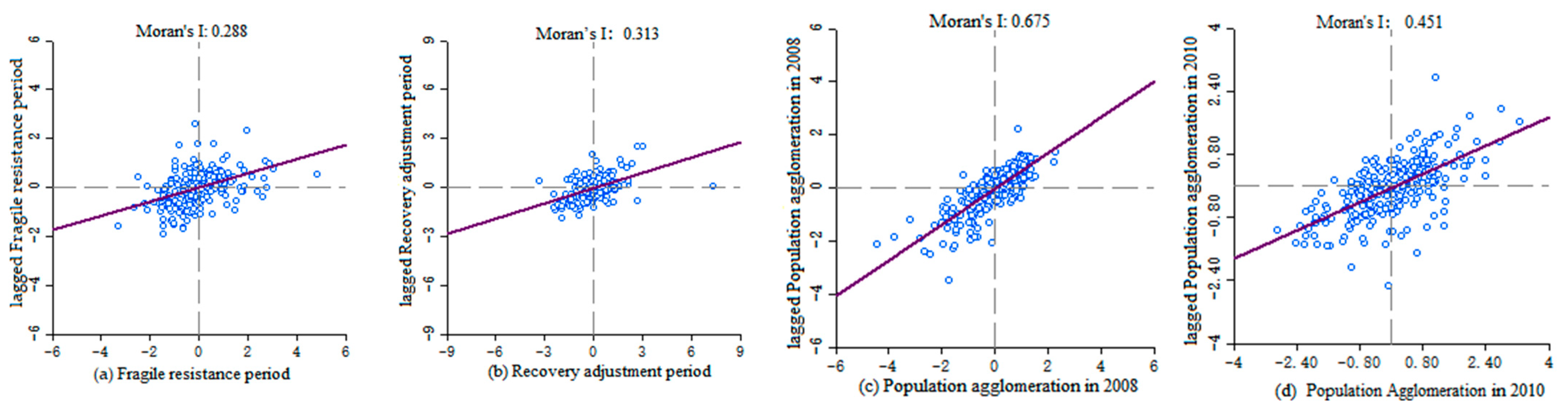
4.2. Spatial Correlation Features

In order to analyze spatial correlations between urban economic resilience and population agglomeration in China, the spatial correlations of urban economic resilience, economic resilience of secondary and tertiary industries and population agglomeration in China were data analysis using GeoDa software to derive the relevant Moran’s I (

Table 3. Moran’s I of urban economic resilience and population agglomeration.

Period	Variable	Moran’s I
Fragile resistance period	Economic resilience	0.288 ***
	Secondary industry economic resilience	0.450 ***
	Tertiary Industry Economic Resilience	0.203 ***
Recovery adjustment period	Economic resilience	0.313 ***
	Secondary industry economic resilience	0.494 ***
	Tertiary Industry Economic Resilience	0.431 ***
Population agglomeration	2008	0.675 ***
	2010	0.451 ***

Note: *** significant at the 1% level.

). Table 3 showed that urban economic resilience, secondary economic resilience, and tertiary economic resilience had significant positive spatial autocorrelation characteristics during the period of fragile resistance and recovery and adjustment period. Spatially exhibit high (low) economic resilience urban agglomeration distribution. Compared with the fragile resistance period, the Moran’s I economic toughness during the economic recovery and adjustment period had been slightly strengthened, indicating that the overall economic resilience index had a clear spatial convergence and strengthening trend. The Moran’s I of the urban population agglomeration in 2008 and 2010 was 0.675 and 0.416, and it passed the 1% significance test, indicating that urban population agglomeration also showed a significant spatial agglomeration trend.

In this study, the local Moran’s I was constructed to describe spatial correlations between economic resilience and population agglomeration in the region and to map a dispersion (Figure 4). Calculations of the global Moran’s I and local Moran index showed that the economic resilience of Chinese cities had a strong spatial correlation and might have spatial spillover effects. Cities with weak economic resilience are less resilient in times of crisis and less able to recover and adjust. This negative change may spread to surrounding cities through recent relationships between cities. However, cities with strong economic resilience are better able to withstand international financial crises and recover and adjust their economies. That is, they can promote their economic development and also drive the economic development of surrounding cities, thereby improving the level of economic resilience. In addition, the spatial correlation of population agglomeration is high and has a spillover effect, and cities’ economic resilience may be affected by the concentration of people in other cities. To make the model result considerably rigorous, spatial spillovers in the model should be considered and the effect of population agglomeration on the economic resilience of cities must be analyzed.

5. Results

Assumptions were used as bases in constructing a model from three aspects to analyze the impact of population agglomeration on economic resilience. First, this paper analyzed whether or not population agglomeration could improve the ability of cities to absorb and withstand economic crises amidst international financial crises, discussed the influence of population agglomeration on the ability of urban economic recovery and adjustment, and discussed whether or not there were differences in the effect of population agglomeration on the economic resilience of urban secondary and tertiary industries. Second, this research started from the working population structure and specifically analyzed the impact of working-age population agglomeration and human capital agglomeration on urban economic resilience. Moreover, this paper analyzed SLM, SEM, and SDM as three spatial econometric models; and presented the OLS regression results for comparison. A multicollinearity test was performed on all explanatory variables of the following models. The results showed that the variance inflation factor of each explanatory variable was below 10, indicating no multicollinearity among the variables. The regression results indicated that the goodness-of-fit R² of the following models after considering the spatial correlation of urban economic resilience was higher than that of the OLS regression. In addition, the regression results were markedly accurate, and the spatial term coefficients (rho and lambda values) in the spatial econometric models were significant, indicating that the regression results of the spatial econometric model were ideal. LM-lag and LM-error passed the 1% significance test, indicating that the economic resilience level of cities would be affected by the weighting of neighboring cities. To analyze the spillover effect of population agglomeration on urban economic resilience, spatial lag variables of the core explanatory variables were calculated and added to the SLM model to construct the SDM model.

5.1. Impact of Population Agglomeration on Urban Economic Resilience

Table 4. Regression results of the impact of population agglomeration on urban economic resilience.

Variable	Fragile Resistance Period				Recovery Adjustment Period
	OLS	SLM	SEM	SDM	OLS	SLM	SEM	SDM
lnpop	0.031 **	0.024 *	0.023 *	0.022	0.074 ***	0.052 ***	0.084 ***	0.030 *
	(2.24)	(1.69)	(1.77)	(1.49)	(3.88)	(3.23)	(4.24)	(1.76)
ste	−0.005 ***	−0.004 ***	−0.004 ***	−0.004 ***	−0.003 **	−0.003 **	−0.003 **	−0.003 **
	(−2.98)	(−2.72)	(−2.94)	(−2.69)	(−2.28)	(−2.30)	(−2.35)	(−2.42)
open	0.004 **	0.004 **	0.004 **	0.003 *	0.002	0.002	0.003	0.002
	(2.33)	(2.17)	(2.35)	(2.11)	(1.26)	(1.59)	(1.63)	(1.54)
lncm	−0.054 *	−0.039	−0.042	−0.037	0.074 *	0.072 **	0.082 **	0.068 *
	(−1.96)	(−1.52)	(−1.64)	(−1.44)	(1.77)	(2.10)	(2.22)	(1.73)
lngdp	0.049	0.026	0.033	0.025	−0.045	−0.072	−0.110 ***	−0.047 *
	(1.42)	(0.80)	(1.04)	(0.76)	(−0.85)	(−1.62)	(−2.74)	(−0.91)
indiv	0.077	0.042	0.055	0.040	0.094	0.142 **	0.175 ***	0.148 **
	(1.47)	(0.79)	(1.12)	(0.76)	(1.21)	(2.19)	(2.79)	(2.09)
fsel	0.007	−0.010	−0.006	−0.016	−0.448 ***	−0.275 ***	−0.432 ***	−0.353 ***
	(0.12)	(−0.16)	(−0.10)	(−0.28)	(−3.96)	(−2.88)	(−3.75)	(−3.34)
W*lnpop				0.0183	−0.182	−0.159	−0.007	0.065 ***
				(0.83)	(−0.74)	(−0.78)	(−0.44)	(2.95)
cons	−0.635	−0.280	−0.402	−0.266		0.151 ***	0.165 ***	−0.273
	(−1.45)	(−0.66)	(−0.99)	(−0.63)		(9.98)	(11.08)	(−1.25)
Ρ/λ		0.388 ***	0.386 ***	0.382 ***	0.074 ***	0.052 ***	0.084 ***	0.445 ***
		(5.32)	(5.46)	(5.22)	(3.88)	(3.23)	(4.24)	(6.77)
N	284	284	284	284	284	284	284	284
R2	0.06	0.18	0.18	0.23	0.11	0.27	0.28	0.28
Log-L		115.590	85.352 ***	115.935		5.933	11.384	3.659
LM-lag/LM-error		91.717 ***	1.373			71.127 ***	76.104 ***
Robustness LM-lag/LM-error		7.738 ***	0.313			0.125	5.102 **

Note: t statistics in parentheses. * Significant at the 10% level, ** significant at the 5% level, *** significant at the 1% level.

showed the regression results of the impact of population agglomeration on urban economic resilience. The results showed that the impact coefficient of population agglomeration was significantly positive during the fragile resistance period, indicating that cities with a high degree of population agglomeration were better able to withstand the shock of an economic crisis. During the recovery adjustment period, the influence coefficient of population agglomeration on urban economic resilience had passed the 1% significance test under the three models of OLS, SLM, and SEM, and the influence coefficient was significantly positive, which was consistent with theoretical expectations, indicating that population agglomeration could significantly improve the city’s ability to recover and adjust the economy after suffering from the international financial crisis. Comparing the estimation results of the models in the two periods, it was found that the population agglomeration coefficient in the recovery and adjustment period model was 2–3 times higher than that in the fragile resistance period, indicating that population agglomeration was of greater significance to the improvement of urban economic resilience during the recovery and adjustment period. In addition, in the SDM model, the coefficient of the spatial lag term of population agglomeration W*lnpop was significantly positive, indicating that the population agglomeration in this city had a positive spillover effect on the economic resilience of surrounding cities. Therefore, suppose H1 was validated.

The regression results of the impact of urban population agglomeration on the economic resilience of the secondary industry (

Table 5. Regression results of the impact of population agglomeration on the economic resilience of the secondary industry.

Variable	Fragile Resistance Period				Recovery Adjustment Period
	OLS	SLM	SEM	SDM	OLS	SLM	SEM	SDM
lnpop	0.096 ***	0.063 **	0.104 **	0.114 ***	0.113 **	0.080 **	0.123 **	0.096 *
	(2.61)	(1.99)	(2.53)	(2.80)	(2.15)	(2.04)	(2.49)	(1.91)
ste	−0.005	−0.004	−0.004	−0.005	−0.005	−0.003	−0.003	−0.004
	(−1.05)	(−0.99)	(−1.02)	(−1.18)	(−1.35)	(−1.20)	(−1.20)	(−1.28)
open	6.66 × 10−5	0.001	−0.001	0.001	0.001	4.48 × 10−4	−0.002	0.001
	(0.01)	(0.25)	(−0.12)	(0.14)	(0.14)	(0.12)	(−0.49)	(0.19)
lncm	−0.065	−0.006	0.016	−0.041	0.232 **	0.116	0.088	0.124
	(−0.87)	(−0.09)	(0.34)	(−0.56)	(2.04)	(1.35)	(0.95)	(1.19)
lngdp	0.127	0.038	0.020	0.082	−0.259	−0.132	−0.087	−0.161
	(1.38)	(0.48)	(0.78)	(0.88)	(−1.77)	(−1.20)	(−0.86)	(−1.17)
indiv	−0.097	−0.111	−0.047	−0.041	−0.258	−0.039	0.190	−0.049
	(−0.69)	(−0.92)	(−0.34)	(−0.29)	(−1.21)	(−0.25)	(1.20)	(−0.24)
fsel	−0.543 ***	−0.441 ***	−0.603 ***	−0.502 ***	−0.761 **	−0.456	−0.747 ***	−0.639 **
	(−3.33)	(−3.16)	(−3.78)	(−3.06)	(−2.46)	(−1.95)	(−2.59)	(−2.22)
W*lnpop				−0.040				0.023
				(−0.70)				(0.32)
cons	−1.058	−0.109	−0.011	−0.632	1.334 **	0.484	−0.019	0.825
	(−0.90)	(−0.11)	(−0.37)	(−0.53)	(1.97)	(0.95)	(−0.45)	(1.27)
Ρ/λ		0.148 ***	0.166 ***	0.213 ***		0.153 ***	0.160 ***	0.477 ***
		(8.73)	(9.34)	(2.63)		(13.71)	(14.21)	(7.76)
N	284	284	284	284	284	284	284	284
R2	0.08	0.17	0.17	0.23	0.05	0.41	0.42	0.43
Log-L		−145.040	−140.918	−173.418		−251.737	−249.363	−295.782
LM-lag/LM-error		51.538 ***	50.707 ***			157.731 ***	150.668 ***
Robustness LM-lag/LM-error		1.143	0.312			7.727 ***	0.664

Note: t statistics in parentheses. * Significant at the 10% level, ** significant at the 5% level, *** significant at the 1% level.

) showed that the impact coefficients of population agglomeration on the urban fragile resistance period and the recovery and adjustment of economic resilience were significantly positive, it showed that urban population agglomeration could not only make the secondary industry develop stably in the face of the international financial crisis, but also improved the recovery and adjustment ability of the secondary industry after the crisis. This was consistent with the expected assumption.

Table 6. Regression results of the impact of population agglomeration on the economic resilience of the tertiary industry.

Variable	Fragile Resistance Period				Recovery Adjustment Period
	OLS	SLM	SEM	SDM	OLS	SLM	SEM	SDM
lnpop	0.009	0.003	0.009	0.020	0.115 ***	0.079 ***	0.099 ***	0.107 ***
	(0.22)	(0.10)	(0.25)	(0.47)	(4.94)	(4.33)	(4.46)	(4.85)
ste	−0.005	−0.004	−0.005	−0.005	−0.001	−0.001	−0.002	−0.0013
	(−1.10)	(−0.99)	(−1.08)	(−1.13)	(−0.85)	(−0.83)	(−1.46)	(−0.98)
open	0.006	0.005	0.006	0.006	−0.001	−3.32 × 10−4	−1.66 × 10−4	2.15 × 10−4
	(1.33)	(1.06)	(1.33)	(1.36)	(−0.30)	(−0.19)	(−0.09)	(0.11)
lncm	−0.396 ***	−0.368 ***	−0.413 ***	−0.412 ***	−0.166 ***	−0.141 ***	−0.172 ***	−0.163 ***
	(−5.18)	(−5.42)	(−5.45)	(−5.36)	(−3.28)	(−3.60)	(−4.15)	(−3.65)
lngdp	0.396 ***	0.383 ***	0.418 ***	0.418 ***	0.174 ***	0.158 ***	0.217 ***	0.156 ***
	(4.16)	(4.54)	(4.47)	(4.31)	(2.68)	(3.14)	(4.81)	(2.63)
indiv	0.346 *	0.272 *	0.348 *	0.332 *	−0.017	−0.064	−0.004	−0.030
	(2.38)	(2.10)	(2.45)	(2.26)	(−0.18)	(−0.87)	(−0.05)	(−0.33)
fsel	0.623 ***	0.469 **	0.624 ***	0.619 ***	−0.715 ***	−0.305 ***	−0.363 ***	−0.370 ***
	(3.71)	(3.12)	(3.79)	(3.61)	(−5.19)	(−2.75)	(−2.82)	(−2.88)
W*lnpop				−0.031				−0.066 **
				(−0.54)				(−2.04)
cons	−4.971 ***	−4.709 ***	−5.293 ***	−5.179 ***	0.424	0.140	1.19 × 10−4	0.380
	(−4.11)	(−4.39)	(−4.43)	(−4.25)	(1.41)	(0.60)	(0.01)	(1.35)
Ρ/λ		0.161 ***	−0.003	0.0771		0.151 ***	0.172 ***	0.524 ***
		(6.92)	(−0.96)	(0.82)		(12.69)	(15.25)	(8.45)
N	284	284	284	284	284	284	284	284
R2	0.13	0.16	0.16	0.20	0.18	0.40	0.39	0.40
Log-L		−164.894	−185.248	−185.184		−29.586	−20.604	−60.421
LM-lag/LM-error		22.487 ***	25.954 ***			117.480 ***	107.829 ***
Robustness LM-lag/LM-error		0.587	4.053 **			10.780 ***	1.129

Note: t statistics in parentheses. * Significant at the 10% level, ** significant at the 5% level, *** significant at the 1% level.

showed the regression results of the impact of urban population agglomeration on the economic resilience of the tertiary industry. During the fragile resistance period, the impact of population agglomeration on the economic resilience of the tertiary industry did not show significance, but the impact coefficients were all positive. The possible reason was that the impact of the 2008 financial crisis on the tertiary industry mainly focused on foreign trade-related industries, and population agglomeration mainly affected domestic demand, so the effect of population agglomeration on the tertiary industry’s resistance to the economic crisis was not significant. During the recovery and adjustment period, the influence coefficient of population agglomeration was significantly positive, indicating that population agglomeration could significantly improve the tertiary industry’s ability to restore and adjust the economy after the international financial crisis. However, the coefficient of the spatial lag term W*lnpop of population agglomeration in the SDM model during the recovery adjustment period was significantly negative, indicating that population agglomeration in this city had a negative spillover effect on the economic resilience of the tertiary industry in surrounding cities. The possible reason was that urban population agglomeration promotes the expansion of the local consumer market to form a scale effect, which had a “siphon” effect on the tertiary industry in surrounding cities, which had an adverse impact on the economic resilience of surrounding cities. Therefore, suppose H1was validated.

5.2. Impact of Labor Structure on Urban Economic Resilience

5.2.1. Impact of Labor Force Age Structure Status on Urban Economic Resilience

Table 7. Regression results of the impact of working-age population agglomeration on economic resilience.

Variable	Fragile Resistance Period				Recovery Adjustment Period
	OLS	SLM	SEM	SDM	OLS	SLM	SEM	SDM
youth	−0.036 **	−0.025 **	−0.027 *	−0.032 **	−0.019	−0.048 **	−0.064 ***	−0.033
	(−2.25)	(−1.99)	(−1.87)	(−2.04)	(−0.72)	(−2.22)	(−2.61)	(−1.27)
prime	0.087 **	0.061 *	0.061 *	0.076 *	0.054	0.129 **	0.173 ***	0.089
	(2.06)	(1.87)	(1.66)	(1.85)	(0.79)	(2.30)	(2.73)	(1.30)
elder	−0.046 *	−0.036 **	−0.035 *	−0.042 *	−0.015	−0.060 *	−0.080 **	−0.034
	(−1.93)	(−1.97)	(−1.73)	(−1.83)	(−0.39)	(−1.92)	(−2.33)	(−0.90)
ste	−0.004**	−0.002	−0.002	−0.002	−0.004 **	−0.003 **	−0.003	−0.003 **
	(−2.07)	(−1.51)	(−1.22)	(−1.40)	(−2.40)	(−2.00)	(−1.88)	(−2.05)
open	0.005 ***	0.004 ***	0.004 **	0.004 **	0.002	0.003 *	0.003 *	0.002
	(2.63)	(2.92)	(2.29)	(2.44)	(1.07)	(1.66)	(1.78)	(1.36)
lncm	−0.056 **	−0.025	−0.022	−0.042	0.087 **	0.074 **	0.103 ***	0.069 *
	(−2.01)	(−1.18)	(−1.39)	(−1.62)	(2.05)	(2.14)	(2.79)	(1.66)
lngdp	0.070 **	0.016	0.009	0.043	−0.033	−0.056	−0.118 ***	−0.033
	(2.00)	(0.58)	(1.03)	(1.29)	(−0.60)	(−1.24)	(−2.90)	(−0.61)
indiv	0.056	0.009	−0.007	0.034	0.067	0.126 *	0.088	0.123
	(1.09)	(0.21)	(−0.16)	(0.65)	(0.84)	(1.94)	(1.46)	(1.53)
fsel	−0.029	−0.036	−0.042	−0.041	−0.347 ***	−0.239 **	−0.318 ***	−0.325 ***
	(−0.46)	(−0.74)	(−0.76)	(−0.69)	(−3.04)	(−2.56)	(−2.88)	(−2.87)
W*youth				−0.023				0.077
				(−0.68)				(1.38)
W*prime				0.055				−0.198
				(0.67)				(−1.44)
W*elder				−0.022				0.114
				(−0.50)				(1.59)
cons	−0.899 **	−0.114	−0.003	−0.514	−0.384	−0.305	−0.007	−0.394
	(−2.04)	(−0.33)	(−0.32)	(−1.21)	(−1.54)	(−1.51)	(−0.44)	(−1.55)
Ρ/λ		0.176 ***	0.175 ***	0.403 ***		0.161 ***	0.165 ***	0.299 ***
		(12.56)	(13.02)	(5.62)		(10.59)	(11.61)	(4.00)
N	284	284	284	284	284	284	284	284
R2	0.06	0.19	0.19	0.25	0.08	0.26	0.28	0.26
Log-L		163.421	163.795	118.425		4.507	7.461	−30.061
LM-lag/LM-error		97.533 ***	92.833 ***			75.099 ***	78.894 ***
Robustness LM-lag/LM-error		5.337**	0.638			0.213	4.008 **

Note: t statistics in parentheses. * Significant at the 10% level, ** significant at the 5% level, *** significant at the 1% level.

showed the regression results of labor force agglomeration at different ages on urban economic resilience. The estimated results of youth labor agglomeration and old labor agglomeration in the two periods were significantly negative, but the influence coefficient of prime-age labor agglomeration was significantly positive. It showed that, compared with the young and old labor, the prime-age labor could better ensure the city resisted the economic crisis and could significantly improve the recovery and adjustment ability of the urban economy, which was consistent with the expected results. In addition, comparing the estimation results of the models in the two periods, the coefficient of the prime-age labor force during the recovery and adjustment period was about twice as high as that during the vulnerable resistance period, indicating that the prime-age labor force had a greater role in promoting the urban economic recovery and adjustment capacity.

5.2.2. Impact of Human Capital Agglomeration on Urban Economic Resilience

Table 8. Regression results of the impact of human capital agglomeration on economic resilience.

Variable	Fragile Resistance Period				Recovery Adjustment Period
	OLS	SLM	SEM	SDM	OLS	SLM	SEM	SDM
lnhom	0.063 ***	0.022	0.044 **	0.058 ***	0.063 *	−0.014	−0.044	−0.006
	(3.10)	(1.36)	(1.99)	(2.62)	(1.85)	(−0.48)	(−1.22)	(−0.15)
lnhet	−0.061 **	−0.027	−0.047 *	−0.060 **	0.004	0.075 **	0.141 ***	0.072 *
	(−2.41)	(−1.35)	(−1.86)	(−2.32)	(0.10)	(2.09)	(3.40)	(1.65)
ste	−0.004 ***	−0.003**	−0.003 **	−0.004 **	−0.003 **	−0.003 **	−0.003 ***	−0.003 **
	(−2.77)	(−2.51)	(−2.35)	(−2.52)	(−2.24)	(−2.45)	(−2.78)	(−2.49)
open	0.004 **	0.003 **	0.003 *	0.003 **	0.002	0.002	0.002	0.002
	(2.29)	(2.39)	(1.89)	(2.14)	(1.32)	(1.49)	(1.39)	(1.44)
lncm	−0.050 *	−0.017	−0.012	−0.031	0.072 *	0.063 *	0.058	0.054
	(−1.81)	(−0.77)	(−0.68)	(−1.19)	(1.72)	(1.83)	(1.55)	(1.33)
lngdp	0.060 *	0.007	0.003	0.034	−0.046	−0.068	−0.084 **	−0.047
	(1.75)	(0.28)	(0.31)	(1.03)	(−0.86)	(−1.54)	(−2.06)	(−0.89)
indiv	0.091 *	0.019	0.001	0.056	0.114	0.132 **	0.190 ***	0.135 *
	(1.72)	(0.45)	(0.02)	(1.06)	(1.44)	(2.02)	(3.05)	(1.69)
fsel	0.026	−0.001	−0.006	0.016	−0.412 ***	−0.311 ***	−0.525 ***	−0.460 ***
	(0.39)	(−0.02)	(−0.09)	(0.25)	(−3.46)	(−3.15)	(−4.38)	(−3.91)
W*lnhom				−0.026				0.179 ***
				(−0.65)				(2.95)
W*lnhet				0.032				−0.153 **
				(0.77)				(−2.41)
cons	−0.865 **	−0.070	−0.004	−0.487	−0.224	−0.077	−0.008	−0.122
	(−1.99)	(−0.20)	(−0.40)	(−1.15)	(−0.88)	(−0.36)	(−0.47)	(−0.48)
Ρ/λ		0.174 ***	0.179 ***	0.391 ***		0.156 ***	0.168 ***	0.254 ***
		(12.06)	(12.48)	(5.23)		(10.05)	(12.25)	(3.31)
N	284	284	284	284	284	284	284	284
R2	0.07	0.20	0.20	0.25	0.12	0.26	0.28	0.30
Log-L		161.286	162.575	118.156		7.025	14.980	−22.764
LM-lag/LM-error		70.806 ***	70.260 ***			67.873 ***	71.950 ***
Robustness LM-lag/LM-error		2.001	1.455			0.005	4.082 **

Note: t statistics in parentheses. * Significant at the 10% level, ** significant at the 5% level, *** significant at the 1% level.

showed the regression results of homogeneous human capital agglomeration and heterogeneous human capital agglomeration on economic resilience in different periods. Regression results showed that the SDM model had the largest R² value of the four models of fragile resistance period. Hence, it was used as the main analysis object, indicating that the agglomeration of homogeneous human capital could significantly increase the resilience of cities to international financial crises. Meanwhile, the agglomeration of heterogeneous human capital was not conducive to the resilience of cities to international financial crises. The reason was that many cities in China mainly relied on the development of leading industries before the global economic crisis in 2008, and supported local economic development through a large number of resource investments. Similar to the construction of “specialized cities”, it once became a trend—under which the homogeneous labor force generally has skilled professionals. Accordingly, enterprises with numerous professional and technical employees had a higher development foundation. That is, they had a greater ability to absorb economic shocks and could cope with the short-term downward pressure on the economy. Hence, cities could continue to maintain high-level development during crises. However, heterogeneous human capital was generally concentrated in cities with high-level economic development. These cities faced significant economic shocks and low economic resilience. Some cities had low-level economic development during international financial crises and could not fully absorb heterogeneous human capital, thereby leading to the misallocation of human capital, which adversely affected the resistance to economic crises. Contrary to the fragile resistance period, the regression results showed that heterogeneous human capital agglomeration with a high education level in the recovery adjustment period could significantly improve cities’ ability to recover and adjust the economy. Therefore, the results validated H3.

6. Discussion and Conclusions

This study took 284 prefecture-level cities in China as the research object to analyze the spatial and temporal distribution characteristics of urban economic resilience and population agglomeration in the context of the 2008 international financial crisis, and on this basis, used a spatial econometric model to empirically analyze the impact of China’s population agglomeration on urban economic resilience.The conclusions of the article are as follows. After the 2008 financial crisis, most cities in China showed a high level of resilience; the differences in urban economic resilience within provinces were small, and the number of highly resilient cities in the eastern region was slightly higher than that in the central and western regions during the fragile resistance period; during the recovery and adjustment period, the differences in urban economic resilience between the north and the south were widened. There are significantly more cities with high economic resilience in the southern region than in the northern region; the urban economic resilience has significant spatial autocorrelation in the two periods. The empirical results showed that cities with high population agglomeration could better withstand the impact of an economic crisis, and could significantly improve the city’s ability to recover and adjust the economy after the crisis. According to the regression results, population agglomeration was of greater significance to the economic resilience of cities during the recovery and adjustment period, and the impact had a positive spillover effect; furthermore, population agglomeration could significantly improve the economic resilience of urban secondary and tertiary industries. To further explore the impact mechanism of population agglomeration on urban economic resilience, this paper analyzed the impact of labor force age structure and quality structure on urban economic resilience under the background of population agglomeration. The specific results were as follows: in terms of labor force age structure, agglomeration of prime-age labor was more important for urban economic resilience than young and old labor; in terms of labor force quality structure, homogeneous human capital significantly improved the city’s resistance to economic crises. The agglomeration of human capital had a significant role in promoting economic resilience during the recovery and adjustment period of cities. In summary, population agglomeration is of great significance for improving urban economic resilience.

From the above conclusions, we can see that China’s good resilience performance under the impact of the 2008 financial crisis is inseparable from the support of its huge population resources. However, in the context of globalization, more external shocks such as climate disasters and public health events have put forward higher requirements for urban economic resilience. Some cities should consider improving economic resilience from the perspective of population agglomeration. First, cities should propose population agglomeration goals and plans based on their industrial structure and development characteristics. Secondly, some cities need to further improve and implement the talent introduction policy, such as actively increasing employment opportunities for foreigners, providing housing subsidies for migrants, and ensuring that migrants and locals have equal rights in infrastructure such as medical education and so on. Finally, the improvement of urban economic resilience is inseparable from the accumulation of human capital. The government can increase the accumulation of various types of talents in cities by increasing investment in education, reforming the education system, and promoting the reform of the vocational education system. Fundamentally provide an impetus for urban development and improve urban resilience.

Although this paper discusses the impact of population agglomeration on urban economic resilience at various stages based on relevant theories and uses existing data to empirically analyze the relationship between urban population agglomeration and urban economic resilience in China, there are still some deficiencies: First, due to a lack of data, it is difficult to empirically test all Chinese cities. Secondly, the article’s measurement of economic resilience is based on the relevant research of scholars at this stage, and it is still necessary to discuss the resilience measurement method suitable for China’s national conditions. In the end, this study only analyzes the influence of population agglomeration on urban resilience from a macroscopic perspective, but the development trajectories and trends of each city are different. There is a need for subsequent studies to analyze the impact of population agglomeration on economic resilience in the context of specific cities.

References

1. Fan, C.C. Interprovincial Migration, Population Redistribution, and Regional Development in China: 1990 and 2000 Census Comparisons. Prof. Geogr. 2005, 57, 295–311. [Google Scholar] [CrossRef]
2. Hudson, R. Resilient regions in an uncertain world: Wishful thinking or a practical reality? Camb. J. Reg. Econ. Soc. 2010, 3, 11–25. [Google Scholar] [CrossRef]
3. Martin, R. Regional economic resilience, hysteresis and recessionary shocks. J. Econ. Geogr. 2012, 12, 1–32. [Google Scholar] [CrossRef]
4. Martin, R.; Sunley, P. On the notion of regional economic resilience: Conceptualization and explanation. J. Econ. Geogr. 2015, 15, 1–42. [Google Scholar] [CrossRef] [Green Version]
5. Lewis, A. Economic Development with Unlimited Supplies of Labour. Manch. Sch. Econ. Soc. Stud. 1954, 22, 139–191. [Google Scholar] [CrossRef]
6. Heberle, R. The Causes of Rural-Urban Migration a Survey of German Theories. Am. J. Sociol. 1938, 43, 932–950. [Google Scholar] [CrossRef]
7. Lee, E. A theory of migration. Demography 1966, 3, 47–57. [Google Scholar] [CrossRef]
8. Mabogunje, A.L. Systems Approach to a Theory of Rural-Urban Migration. Geogr. Anal. 1970, 2, 1–18. [Google Scholar] [CrossRef]
9. Davies, S. Regional resilience in the 2008–2010 downturn: Comparative evidence from European countries. Camb. J. Reg. Econ. Soc. 2011, 4, 369–382. [Google Scholar] [CrossRef]
10. Faggian, A.; Gemmiti, R.; Jaquet, T.; Santini, I. Regional economic resilience: The experience of the Italian local labor systems. Ann. Reg. Sci. 2018, 60, 393–410. [Google Scholar] [CrossRef]
11. Capello, R.; Caragliu, A.; Fratesi, U. Spatial heterogeneity in the costs of the economic crisis in Europe: Are cities sources of regional resilience? J. Econ. Geogr. 2015, 15, 951–972. [Google Scholar] [CrossRef]
12. Huang, X. Immigration and economic resilience in the Great Recession. Urban Stud. 2021, 58, 1885–1905. [Google Scholar] [CrossRef]
13. Becker, G.S. Investment in Human Capital: A Theoretical Analysis. J. Political Econ. 1962, 70, 9–49. [Google Scholar] [CrossRef]
14. Storper, M.; Scott, A.J. Rethinking human capital, creativity and urban growth. J. Econ. Geogr. 2009, 9, 147–167. [Google Scholar] [CrossRef] [Green Version]
15. Niebuhr, A. Migration and innovation: Does cultural diversity matter for regional R&D activity? Pap. Reg. Sci. 2010, 89, 563–585. [Google Scholar]
16. Giannakis, E.; Bruggeman, A. Regional disparities in economic resilience in the European Union across the urban-rural divide. Reg. Stud. 2020, 54, 1200–1213. [Google Scholar] [CrossRef]
17. Zaiceva, A.; Zimmermann, K.F. Migration and the Demographic Shift. Handb. Econ. Popul. Aging 2016, 1, 119–177. [Google Scholar]
18. Bodvarsson, R.B.; Simpson, N.B.; Sparber, C. Migration Theory. Handb. Econ. Int. Migr. 2015, 1, 3–51. [Google Scholar]
19. Gobel, C.; Zwick, T. Are personnel measures effective in increasing productivity of old workers? Labour Econ. 2013, 22, 80–93. [Google Scholar] [CrossRef]
20. Borsch-Supan, A.; Weiss, M. Productivity and age: Evidence from work teams at the assembly line. J. Econ. Ageing 2016, 7, 30–42. [Google Scholar] [CrossRef] [Green Version]
21. Sanchez-Zamora, P.; Gallardo-Cobos, R. Diversity, Disparity and Territorial Resilience in the Context of the Economic Crisis: An Analysis of Rural Areas in Southern Spain. Sustainability 2019, 11, 1743. [Google Scholar] [CrossRef] [Green Version]
22. Luo, Y.; Wang, Y.; Fan, Z.J. Heterogeneous Human Capital, Regional Specialization and Income Disparity—From the Perspective of New Economic Geography. China Ind. Econ. 2013, 2, 31–43. [Google Scholar]
23. Diodato, D.; Weterings, A.B.R. The resilience of regional labour markets to economic shocks: Exploring the role of interactions among firms and workers. J. Econ. Geogr. 2015, 15, 723–742. [Google Scholar] [CrossRef]
24. Caroli, E.; Van Reenen, J. Skill-biased organizational change? Evidence from a panel of British and French establishments. Q. J. Econ. 2001, 116, 1449–1492. [Google Scholar] [CrossRef]
25. Ciccone, A.; Papaioannou, E. Human Capital, The Structure of Production, and Growth. Rev. Econ. Stat. 2009, 91, 66–82. [Google Scholar] [CrossRef]
26. Juster, F.T. Education, Income, and Human Behavior; McGraw-Hill Book Company: Hightstown, NJ, USA, 1975. [Google Scholar]
27. Marais, M.A. The Consumption Benefits of Education; Economics Discussion; The University of Western Australia, Department of Economics: Perth, Australia, 1993. [Google Scholar]
28. Liu, R.; Feng, Z.; Yang, Y.; You, Z. Research on the Spatial Pattern of Population Agglomeration and Dispersion in China. Prog. Geogr. 2010, 29, 1171–1177. [Google Scholar]
29. Brown, L.; Greenbaum, R.T. The role of industrial diversity in economic resilience: An empirical examination across 35 years. Urban Stud. 2017, 54, 1347–1366. [Google Scholar] [CrossRef]
30. Zhang, M.D.; Wu, Q.B.; Li, W.L.; Sun, D.Q.; Huang, F. Intensifier of urban economic resilience: Specialized or diversified agglomeration? PLoS ONE 2021, 16, e0260214. [Google Scholar] [CrossRef]
31. Tan, J.T.; Hu, X.H.; Hassink, R.; Ni, J.W. Industrial structure or agency: What affects regional economic resilience? Evidence from resource-based cities in China. Cities 2020, 106, 102906. [Google Scholar] [CrossRef]
32. Christopherson, S.; Michie, J.; Tyler, P. Regional resilience: Theoretical and empirical perspectives. Camb. J. Reg. Econ. Soc. 2010, 3, 3–10. [Google Scholar] [CrossRef]
33. Yu, H.C.; Liu, Y.; Liu, C.L.; Fan, F. Spatiotemporal Variation and Inequality in China’s Economic Resilience across Cities and Urban Agglomerations. Sustainability 2018, 10, 4754. [Google Scholar] [CrossRef] [Green Version]
34. Boschma, R. Towards an Evolutionary Perspective on Regional Resilience. Reg. Stud. 2015, 49, 733–751. [Google Scholar] [CrossRef] [Green Version]
35. Wang, W.L.; Wang, J.L.; Wulaer, S.; Chen, B.; Yang, X.D. The Effect of Innovative Entrepreneurial Vitality on Economic Resilience Based on a Spatial Perspective: Economic Policy Uncertainty as a Moderating Variable. Sustainability 2021, 13, 10677. [Google Scholar] [CrossRef]
36. Duranton, G.; Puga, D. Diversity and specialisation in cities: Why, where and when does it matter? Urban Stud. 2000, 37, 533–555. [Google Scholar] [CrossRef] [Green Version]
Figure 1. Impact of population agglomeration on urban economic resilience.
Sustainability 14 10407 g001
Figure 2. China’s GDP growth rate.
Sustainability 14 10407 g002
Figure 3. Spatial distribution of urban economic resilience and population agglomeration in different periods in China. (a) shows the distribution map of China’s urban economic resilience during the fragile resistance period, (b) shows the distribution map of China’s urban economic resilience during the recovery and adjustment period, (c) shows the relationship between urban economic resilience and population agglomeration during the fragile resistance period, and (d) shows the relationship between urban economic resilience and population agglomeration during the recovery and adjustment period. Note: The map is based on the standard map downloaded from the standard map service website of the Ministry of Natural Resources (the approval number is GS (2020)4632), and the base map has not been modified.
Sustainability 14 10407 g003
Figure 4. Moran index dot plot of economic resilience and spatial distribution of population agglomeration in Chinese cities. As shown in Figure 4, the number of cities with urban economic resilience in the first quadrant (HH type) had decreased from 110 in the fragile resistance period (a) to 105 in the recovery adjustment period (b), and the distance closed to the coordinate axis has shortened, indicating that the distribution of high-resilience cities in the recovery and adjustment period is shrinking. The number of cities included in the third quadrant (type LL) had decreased from 93 in the fragile resistance period to 90 in the recovery adjustment period and was also concentrated near the coordinate axis. The number of cities distributed in the second quadrant (LH type) and the fourth quadrant (HL type) was small in the fragile resistance period and the recovery and adjustment period and the number of cities did not change significantly. In 2008 (c) and 2010 (d), the local Moran index scatter plot distribution of urban population agglomeration was basically consistent with the distribution trend of urban economic resilience. Most cities were still concentrated in the first quadrant (HH type) and the third quadrant (LL type), with significant spatial correlation.
Sustainability 14 10407 g004