1. Introduction
Behavioural choices are influenced by needs, opportunities, and skills [
1]. In addition, the demand for products and services to meet population needs results from behavioural decisions. Consumption relationships are closely related to the freight demand, which influences urban freight transport (UFT) planning. However, UFT planning is challenging, as demand is not always known, and surveys to obtain data are expensive. Freight demand modelling can then be used to support UFT planning.
Furthermore, cargo movements are much more complex than passenger transport given that cargo movements involve interactions between companies at different supply chain stages [
2] and different stakeholders and decision makers throughout the process. However, those who should plan urban transport policies usually lack a detailed view of the complex factors that influence UFT [
2]. Thus, several problems (e.g., congestion, noise, visual and atmospheric pollution, safety, and damage to the infrastructure) are reflections of the lack of sustainable planning and operation [
3,
4,
5]. UFT directly affects the product cost.
In order to understand UFT as a complex phenomenon, Cassiano et al. [
6] proposed a conceptual model to represent the operation of the last mile in urban areas. The model focused on impact measures that were capable of guiding decision-makers toward sustainable UFT. In addition, this model was based on (1) the relationship between urban activities’ subsystems and the transport subsystem, and (2) on how this relationship impacts UFT operation and consequently the stakeholders. The model proposed by Cassiano et al. changes the classic idea of reducing the urban environment to the space where the freight trip generation process takes place. The framework in Cassiano et al. considers three major steps: UFT starts in the purchase process from the urban activities’ subsystem, moves around the transportation system with the freight trip generation model, and reaches the destination. Therefore, freight transport models are important and can be used to plan freight policies [
7]. Furthermore, understanding the movements of goods is essential to supporting sustainable planning.
However, freight transport modelling is still in the early stages of development in many developing countries [
8]. For example, in Brazil, freight trip generation models (FTGM) were estimated for some economic sectors, such as pubs and restaurants [
9,
10], supermarkets [
10], shopping centres [
9], buildings under construction [
11], and warehouses [
12]. Moreover, FTGM were used to evaluate parking needs in historical city centres [
13] and freight trip flows in urban areas [
14]. As a consequence of the lack of knowledge related to freight movements, freight policies are flawed and do not address freight problems [
15]. Therefore, modelling efforts are needed to support freight policies. However, the lack of data, political priorities, and the slow pace of the knowledge-building process are some of the reasons for these limited research efforts [
8]. This context, which is described by authors in India, is similar in Brazil.
UFT planning in Brazil is neglected by transportation authorities and planning agencies. Furthermore, freight transport is considered a private activity with limited impacts on the local economy. However, freight transport is of great importance for economic development. Creating knowledge and showing the impact of cargo movements in Brazilian cities are important to include this activity in urban planning.
To the best of the authors’ knowledge, no paper has addressed FTGM estimation using deliveries to commercial establishments in Brazilian municipalities, as proposed in this paper. Thus, this paper estimates FTGM considering retail deliveries in Brazilian municipalities, which are based on their administrative and populational characteristics. These differences in administrative and populational characteristics allow dissimilarities between the estimated models to be discussed, which is better for planning freight movements.
Additionally, FTGM are generally estimated using linear regression [
8,
16]. However, this technique has some assumptions that need to be validated to ensure the accuracy of the estimated models. However, few studies have considered these assumptions explicitly in the analysis, especially among the existing Brazilian studies. Thus, a procedure is used to estimate FTGM using ordinary least squares (OLS) regression, and alternative techniques are considered to address the violations of the OLS assumptions. This procedure is shown by estimating FTGM using deliveries to commercial establishments in Brazilian municipalities. Furthermore, this study shows that alternative techniques to linear regression can provide better-estimated parameters and more accurate results.
The contribution of this paper is twofold. First, FTGM are estimated using delivery data, which contributes to understanding freight movements in Brazilian cities. Second, this study shows the importance of evaluating the OLS assumptions in FTGM, which is not always addressed by other studies.
This paper is structured in five sections.
Section 2 presents a review of the FTGM literature and discusses modelling issues for better model accuracy.
Section 3 details the approach used, and an application is shown in
Section 4. The conclusion is presented in
Section 5.
2. Freight Trip Generation Models—The Literature
This paper conducted a systematic literature review to address the research question: “How does the literature address FTGM?”
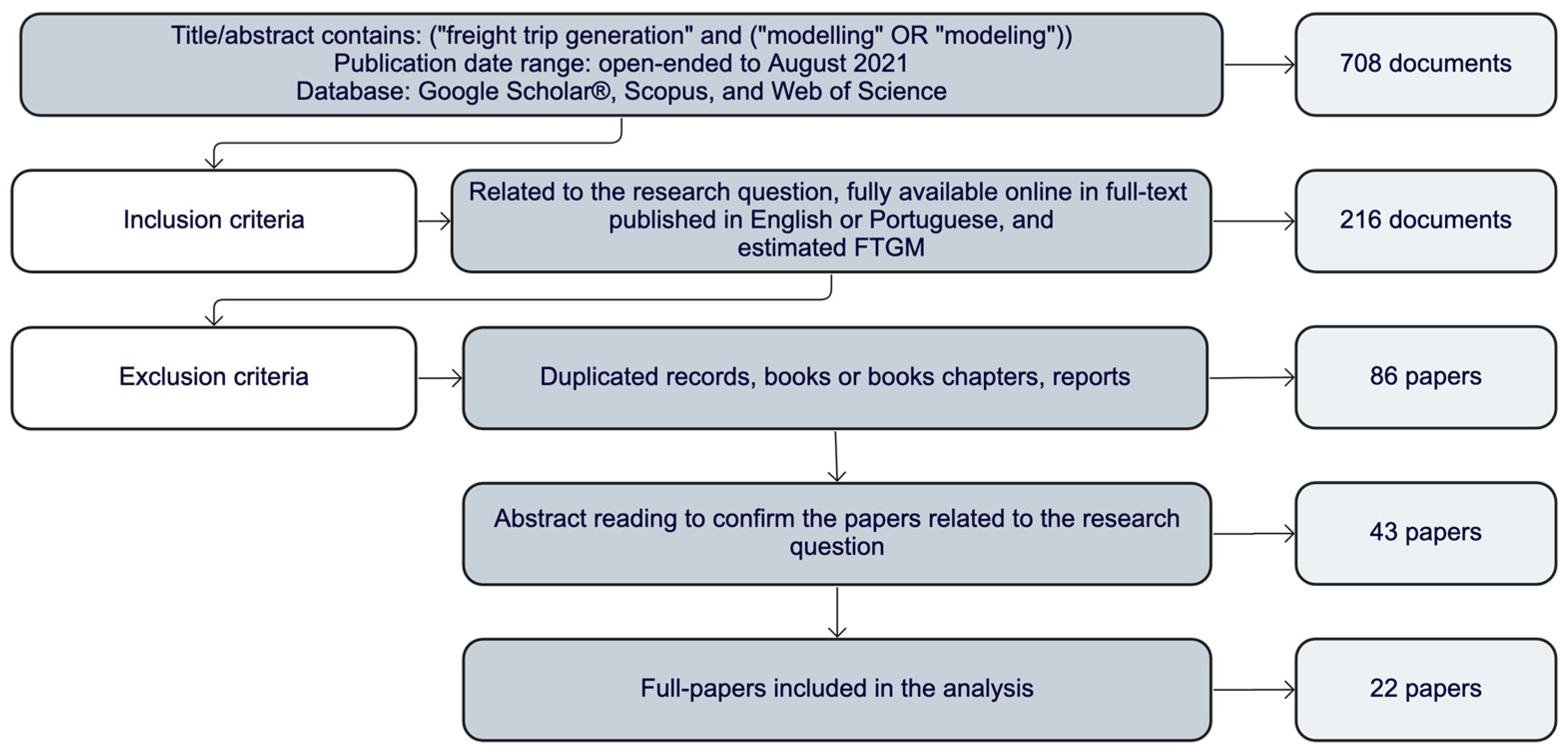
Figure 1 describes the literature selection procedure. Considering this research question, “freight trip generation” and “modelling” were selected as search keywords. The search was conducted in Scopus, Web of Science, and Google Scholar
®. Google Scholar
® was included since the authors knew beforehand that some classical papers would not be found in the other two databases. The search was limited to documents up to August 2021. Then, the search procedure yielded 708 documents: 160 in Scopus, 76 in Web of Science, and 476 in Google Scholar
®. The inclusion criteria considered records (1) that were related to the research question and that estimated FTGM, (2) that were available online in full text, and (3) that were published in English or Portuguese. The exclusion criteria considered books, chapters, reports, and duplicated records. The inclusion and exclusion criteria resulted in 43 papers, whose abstracts were read. Another 21 papers were excluded, which led to 22 remaining papers for the analysis. Lastly, these 22 papers were read, categorised, and analysed.
The literature review was then systematised concerning objectives, techniques, goodness-of-fit measures, and OLS assumptions.
Table 1 summarises the literature.
The OLS is the most used regression technique to estimate FTGM. Moreover, alternative regression models have been used to solve the limitations of the OLS assumptions. Examples include generalised linear regression [
11,
16,
17,
18], logit or probit models [
17,
19,
20], non-linear regression [
13,
21], negative binomial regression [
22,
23,
24], and spatial models [
22,
23,
25,
26,
27].
The number of employees and the establishment area are generally the independent variables used to explain FTGM [
11]. In addition, the usual measures for evaluating the models’ goodness-of-fit are the
t-test, the F-test, and the R-squared. Furthermore, the Akaike information criteria (AIC), the Bayesian information criterion (BIC), the root mean squared error (RMSE), and the mean absolute percentage error (MAPE) are used to compare and measure the accuracy of the models.
The reliability of the OLS estimators is verified by evaluating the OLS assumptions: endogeneity, multicollinearity, linearity of parameters, autocorrelated errors, homoscedasticity, and the normality of the error distribution [
18]. Econometric-related studies have carefully addressed these assumptions, as reported by [
28,
29], and recommended such considerations for transportation data analysis [
30]. However, few studies have evaluated all the OLS assumptions [
16,
31]. Therefore, not evaluating the OLS assumptions compromises the accuracy of the models, which could lead to errors in prediction and thus negatively impact the planning process.
Some papers focused on the role of the urban environment in freight trip movements [
25,
32]. Other studies considered freight trip attraction models using the business characteristics of commercial establishments [
8,
10,
17,
33,
34]. Finally, several studies evaluated parking needs [
13,
16,
35], the relationship between freight trip movements and accessibility [
34], and the role of aggregating commercial establishments by categories [
25,
36]. FTGM can support both planning and public policies, as they can help regulate freight activities and forecast future scenarios [
8,
25,
26,
34,
37].
The literature shows that considerable effort has been made to find the best models to explain FTGM. Moreover, the OLS regression is usually considered to estimate FTMG. However, many researchers have not used suitable techniques to support the associated methodological effort. For example, few studies have evaluated the OLS assumptions when estimating OLS models. Therefore, this paper intends to contribute to this issue by describing the fundamental steps for a reliable trip-generation estimation. This procedure is presented in the next section.
3. Procedure for Estimating FTGM
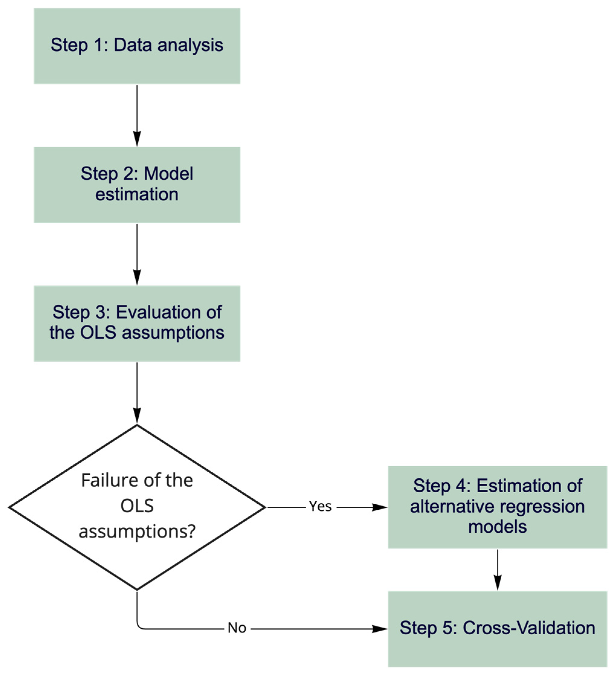
This section describes the procedure used to estimate FTGM. The OLS regression is a classical technique to estimate the coefficients of linear regression models. Such regression is well detailed in the econometric literature since it is a common method to develop theories or to test existing hypotheses. Nonetheless, in the transportation literature, OLS regression is a common procedure that presents some flaws. Thus, this work shows, in a simple way, how to use the classical linear regression theory to estimate FTMG.
Figure 2 presents the steps proposed in this procedure, which are detailed in the next subsections.
This study considered the usual variables in FTGM: The dependent variable (Y) is the number of deliveries per week, and the independent variables are the number of employees (X1) and the establishment areas (X2). However, other variables, if collected, can be used for FTGM. These data were obtained from an establishment-based survey that was conducted in Brazilian cities. Oliveira et al. [
38] presented another study using the same data.
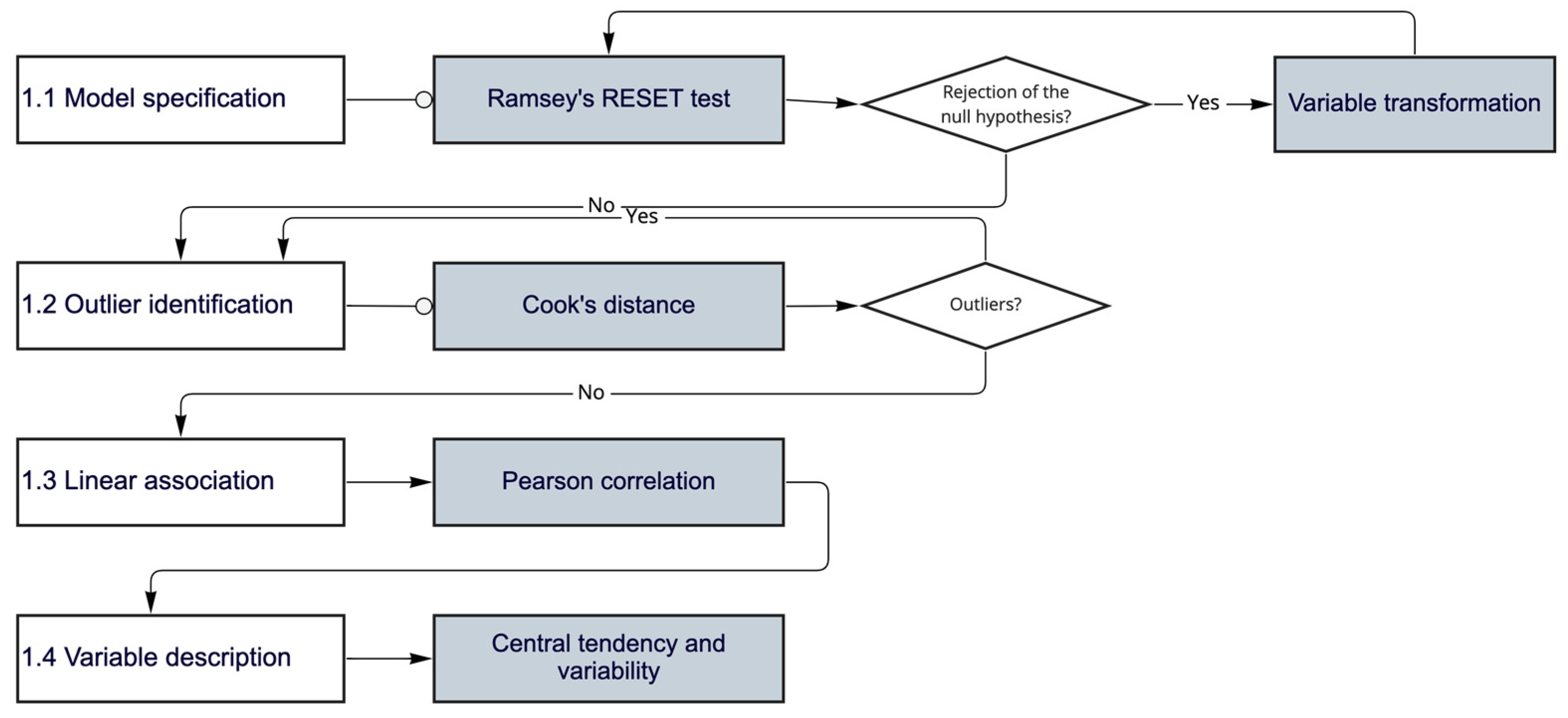
3.1. Step 1: Data Analysis
Figure 3 shows the sub-steps from the data analysis. Step 1.1 is related to the functional form of the linear models (i.e., model specification). A functional form refers to the algebraic formula that establishes a relationship between a dependent variable and the explanatory variables. However, linear regression models may suffer from functional form misspecification [
28]. The Ramsey Regression Equation Specification Error Test (RESET test) proposed by Ramsey [
39] can be used to evaluate the general functional form misspecification. The null hypothesis considers that the functional form is correctly specified, and the rejection of the null hypothesis indicates that the model is misspecified [
28]. The null hypothesis is rejected at a 95% significance level when the
p-value is lower than 0.05. It should be noted that the RESET test is a functional form test; however, a model can also be misspecified due to omitted variables, which might not be identified by the RESET test [
28]. Therefore, it is essential to ensure that the model variables explain the phenomenon well. The lmtest package [
40] in the R environment was used to perform the RESET test.
In a misspecified model, variable transformation is required to identify linear patterns. The most usual variable transformations are presented in
Table 2. After the variable transformation, the RESET test can be used to verify the linear pattern of the functional forms.
Assuming the functional form has been verified, step 1.2 concerns outlier identification, i.e., observations that lie at an abnormal distance from other observations in a random sample. Outliers are generally observed when modelling systems use real data. However, outliers can increase the variation of the explanatory variables and lead to models with lower predictive power. Thus, the decision to keep such observations in a regression analysis can be challenging [
28]. In this study, outliers are removed. Since the data come from information declared by interviewees, the questions may be misinterpreted. In addition, interviewees can answer the questions with inaccurate estimations. For example, respondents presented difficulties getting to know the establishment area. In addition, deliveries are known to fluctuate over time due to bank holiday dates. For this question, the number of deliveries was also an estimate given by the respondents, which was based on their experiences. Considering the size of the available database, removing the outliers would be beneficial to improve model estimation.
Thus, influential outliers were identified by the Cook’s distance. First, the regression model was estimated and the Cook’s distance was calculated to identify the influential observations, i.e., observations with a Cook’s distance greater than four times the average. The influential observations were removed from the sample. The process was repeated as long as there were influential points in the sample. Cook [
41] provides additional details about the mathematical procedure to identify influential measures. The outlier removal process provides the final database for estimating FTGM.
Step 1.3 requires measuring the level of association between the variables by the Pearson correlation coefficient. The correlation level varies from −1 (negative correlation) to +1 (positive correlation). A value below ±0.38 indicates a weak correlation, a value between ±0.4 and ±0.69 indicates a moderate correlation, a value between ±0.7 and ±0.89 indicates a strong correlation, and a value above ±0.9 indicates a very strong correlation. A strong correlation between the independent and the dependent variables is desirable.
Finally, step 1.4 summarises the data by calculating their central tendency and the associated variability.
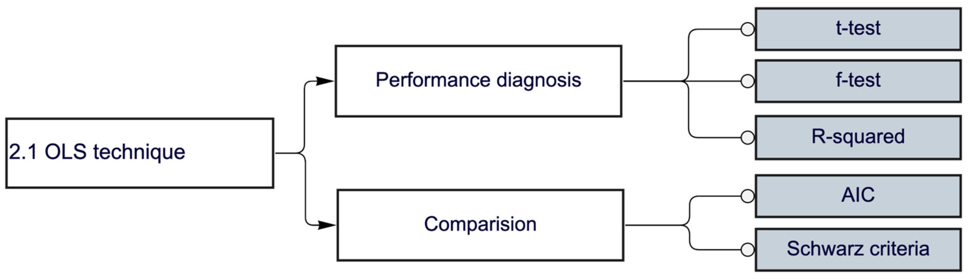
3.2. Step 2: Estimation of the Linear Model
Figure 4 shows the procedures in step 2. The OLS technique was used to estimate the linear models. The functional form of the OLS model is represented by Equation (1), where Y is the dependent variable, X1,…, Xn are the explanatory variables, β1,…, βn are the estimators, εn is the error, and n is the number of observations. The OLS regression minimises the difference between observed and predicted values (i.e., the sum of squared errors).
The goodness-of-fit tests indicate the models’ performance. The usual goodness-of-fit measures are the hypothesis tests of estimators (T-test) and of the model (F-test), and the measure of the model fit (R-squared). The hypothesis tests of the estimators are conducted by the T-test, which identifies the linear association between the estimator and the dependent variable. The F-statistic tests the statistical significance of the independent variables in the linear regression. Moreover, the R-squared measure evaluates the prediction power of the OLS model. These statistics are usually verified in FTGM, as pointed out by the existing literature.
The Akaike information criterion (AIC) and the Bayesian information criterion (BIC) are used for comparing models. The AIC is a measure for scoring, comparing, and selecting the estimated models by different techniques. The model with the smallest AIC is recommended [
42]. The BIC, also called the Schwarz information criterion, is used for selecting econometric models. The model with the lowest BIC is preferred [
43].
3.3. Step 3: Evaluation of the OLS Assumptions
Verifying OLS assumptions avoids incorrect parameter estimation [
18]. Violation of the OLS assumptions results in misuse and inaccurate models. The main classical OLS assumptions are [
29,
30] (i) linearity of the parameters, (ii) uncorrelated regressors and errors, (iii) homoscedasticity, (iv) no autocorrelation between the errors, (v) multicollinearity, and (vi) normally distributed errors.
Figure 5 details the required test to evaluate each of these assumptions.
The linearity assumption (step 3.1) considers a linear pattern of the parameters. The RESET test evaluates the models’ functional form, as explained earlier. Additionally, the response variable Y must be continuous [
30] and positive [
29]. If a linear pattern is not identified, alternative techniques (e.g., non-linear regression model, generalised least-squares, maximum likelihood estimation, Bayesian regression, kernel regression, or gaussian process regression) must be used to estimate the parameters.
The assumption of uncorrelated regressors and errors (Step 3.2) is known as regressor exogeneity. An exogenous regressor is uncorrelated with the random error term, i.e., the regressor has zero variance with the error term. An endogenous regressor is the opposite of an exogenous regressor and is unsuitable for OLS estimation. The Durbin–Wu–Hausman (DWH) test (also called the Hausman specification test) checks exogenous regressors. The null hypothesis assumes an exogenous regressor, and the rejection of the null hypothesis indicates an endogenous regressor. The instrumental variable technique is an alternative to endogenous regressors.
Homoscedasticity or constant error variance is evaluated in step 3.3. Homoscedasticity means constant variance, whereas heteroskedasticity means variance in the errors. The Goldfeld–Quandt test and the Breush–Pagan test check for homoscedasticity. The null hypothesis of the Goldfeld–Quandt test is homoscedasticity, whereas the null hypothesis of the Breush–Pagan test is heteroskedasticity. The rejection of the null hypotheses indicates heteroskedasticity and homoscedasticity, respectively. Thus, it is expected that the null hypothesis of the Goldfeld–Quandt test will not be rejected and that the null hypothesis of the Breush–Pagan test will be rejected. Robust regression can be used to solve the heteroskedasticity problem.
Step 3.4 evaluates the assumption that the residual errors should be independent (i.e., without autocorrelation). The autocorrelation of the error terms is a typical problem in time-series analysis. The Durbin–Watson test is used to evaluate this assumption. The null hypothesis assumes that the residual errors are independent, and the rejection of the null hypothesis indicates autocorrelated errors. Robust regression can be implemented to account for this violation.
Step 3.5 evaluates the multicollinearity assumption between the regressors. Multicollinearity is observed when the variables are correlated, and it implies inaccurate estimation. If multicollinearity is observed, the OLS estimators have no statistical significance. Multicollinearity can be detected by measuring the variance inflation factor (VIF). Alternatively, the Farrar–Glauber test can be used to measure the orthogonality of the variables, and the condition index can be calculated to diagnose this problem. Eliminating variables with VIF > 10 might solve the multicollinearity problem. In addition, combining variables may minimise the multicollinearity problem.
Finally, the assumption of normally distributed errors (step 3.5) is considered. This assumption is not a requirement for estimating linear regression models, but having normally distributed errors is required to make inferences about the model parameters [
30]. The Kolmogorov–Smirnov and the Shapiro–Wilk tests check whether the errors are normally distributed (i.e., null hypothesis). Generalised linear models (GLM) are an alternative for count data, whereas tobit regression can be used for censored data. Moreover, a semi-parametric regression is an alternative for other cases [
44]. More information about the OLS assumptions is provided in [
29].
3.4. Step 4: Estimation of Alternative Regression Models
Violating OLS assumptions requires estimating models by alternative techniques. This paper used two methods due to the violation of OLS assumptions: robust regression and tobit regression.
Robust regression is an alternative to OLS regression with less restrictive assumptions. The residual standard error (RSE) measures the standard deviation of the residuals. A low RSE value indicates that the model fits the data. More information about robust regression can be found in [
45]. Robust regression models were estimated using the MAAS package [
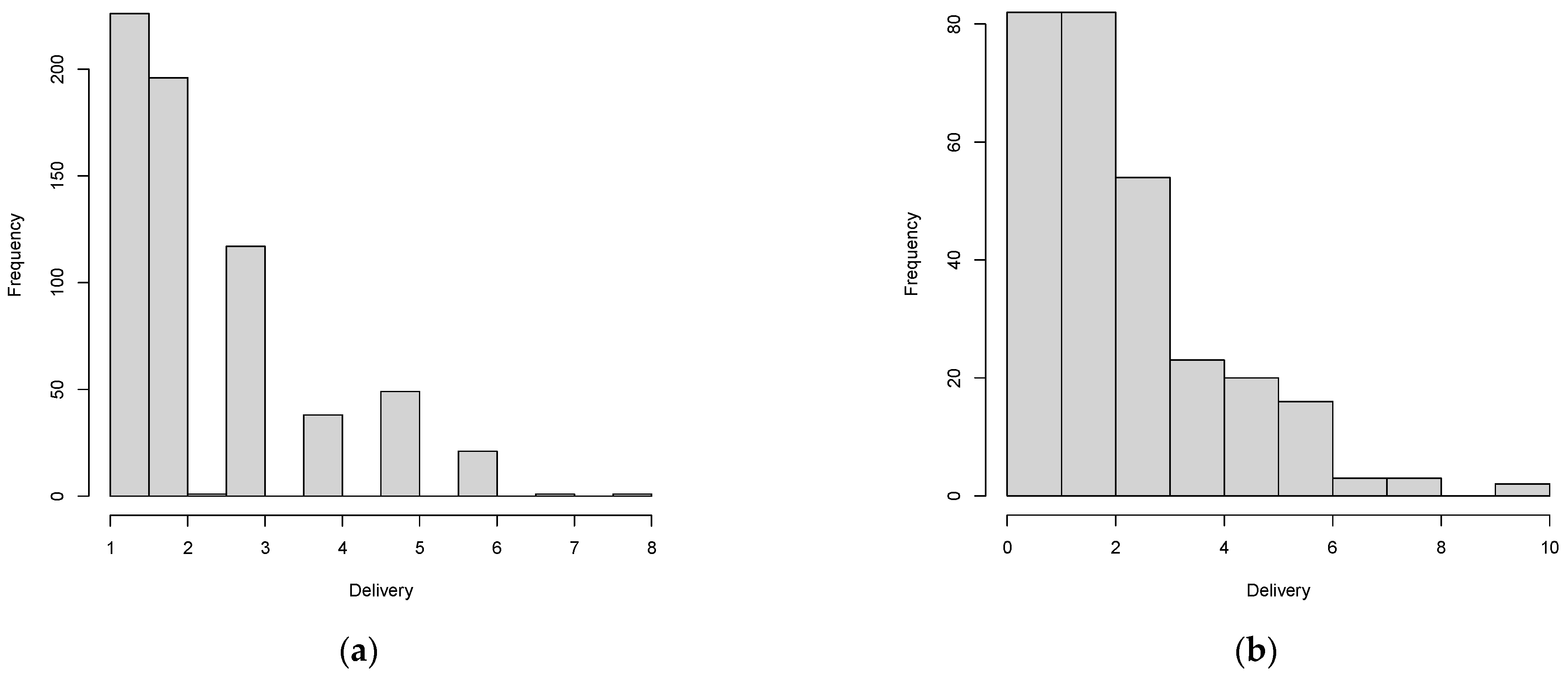
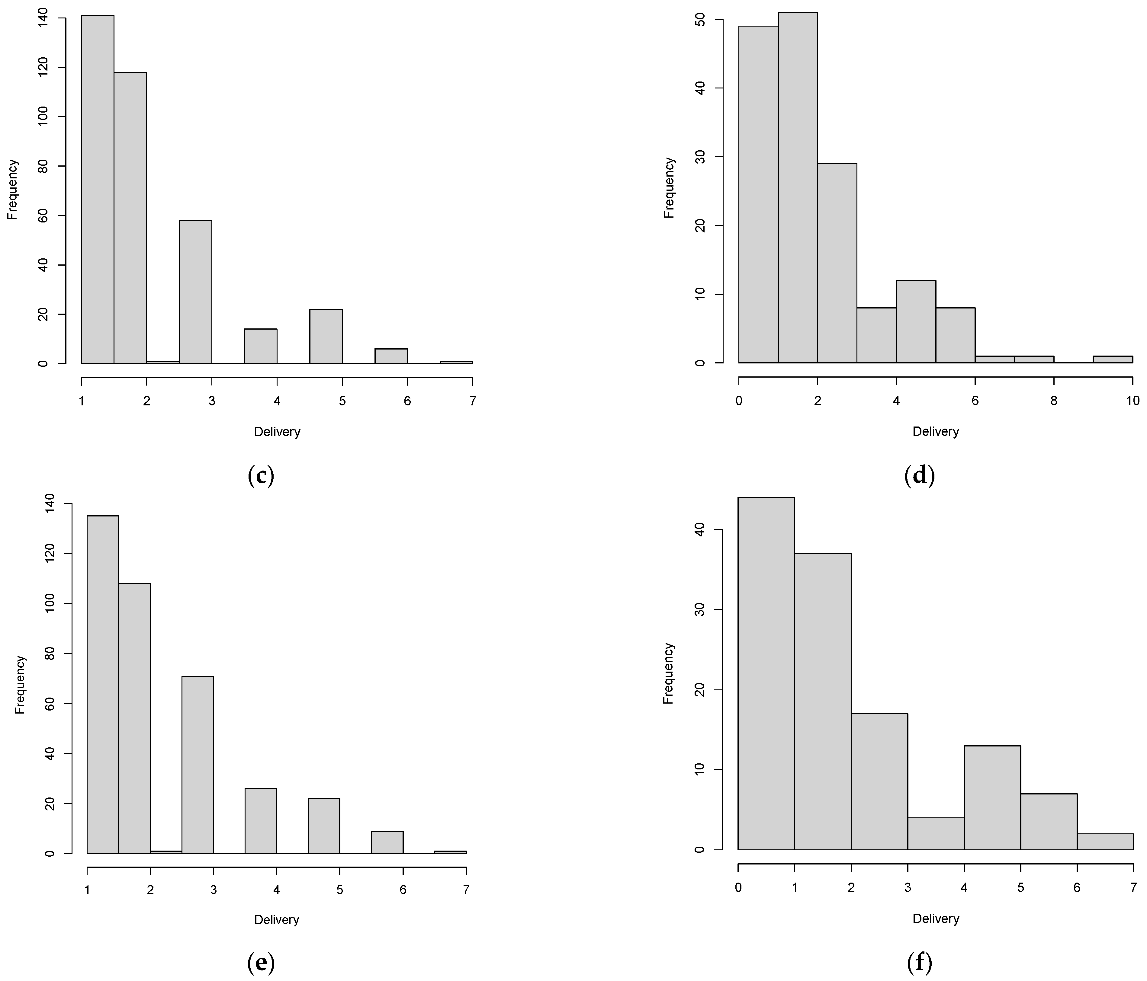
45] in the R environment. Tobit regression is an alternative for censored data and for errors that are not normally distributed. For example,
Figure 6 shows that the explanatory variable delivery is right-censored. Therefore, tobit regression can be used. Wooldridge [
28] details the formulation of the tobit model. Tobit models were estimated using the VGAM package [
46] in the R environment. The statistical significance of the estimated coefficients in both cases was evaluated by the z-value. Finally, the estimated models were compared by AIC and BIC.
3.5. Step 5: Cross-Validation Analysis
Cross-validation measures the model’s predictive performance using test data. Two cross-validation methods were used: leave-one-out cross-validation (LOOCV) and K-fold. LOOCV uses all observations and reduces potential bias. In this case, one data point is left out, and the model is estimated with the rest of the data set. Thus, the model’s predictive power is evaluated using the data point left out and the test error associated with the prediction is recorded. The process is repeated for all data points, which enables the root mean squared error (RMSE) and the mean absolute error (MAE) to be computed. The RMSE is used to measure the difference between observed and predicted values. The MAE is the average of the absolute error values.
In the K-fold procedure, the dataset is split into k-subsets. Thus, one subset (testing data) is selected for testing and the model is estimated with the other subsets (training data). The model is predicted using the testing data, and the prediction error is calculated. This process is repeated until k subsets are used as a testing set. Finally, the RMSE and the MAE are computed.
4. Results
A questionnaire was designed to collect data related to the area of the commercial establishment, the number of employees, and the number of deliveries per week. The researchers visited several commercial establishments and invited the employers to answer the questionnaire. This process resulted in data from 860 commercial establishments from nine Brazilian cities: Belo Horizonte, Betim, Caruaru, Contagem, Divinopolis, Itabira, Nova Lima, Palmas, and Quixada. In the analysis, no distinction was made between the various economic sectors of the commercial establishments. However, we acknowledge the importance of the economic sector for FTGM and plan to address this issue in the future.
Data grouping was used to analyse differences in the models generated for cities with similar characteristics. The administrative and population characteristics were then considered, and the models were estimated for the following subsets: (i) all data; (ii) state capital cities (Belo Horizonte and Palmas); (iii) non-capital cities (Betim, Caruaru, Contagem, Divinopolis, Itabira, Nova Lima, and Quixada); (iv) larger cities, i.e., cities with a population greater than 50,000 inhabitants (Belo Horizonte, Betim, and Contagem); (v) medium cities, i.e., cities with a population between 100,000 and 500,000 inhabitants (Caruaru, Divinopolis, Itabira, and Palmas); and (vi) small cities, i.e., cities with a population lower than 100,000 inhabitants (Nova Lima and Quixada).
Table 3 shows the Ramsey RESET test results to evaluate the functional form. The linear functional form was unsuitable for all subsets, i.e., the null hypothesis of the Ramsey RESET test was rejected, and the functional form was not correctly specified. The log–log functional transformation was suitable for all subsets. Moreover, the linear–log, the inverse, and the log–inverse transformations were suitable for some groups: linear–log functional form for the subsets “all data,” “capital,” “non-capital cities,” and “larger cities”; inverse functional form for the subsets “larger cities,” “medium cities,” and “small cities”; and the log–inverse functional form for the subset “non-capital cities.” The results showed the importance of evaluating the functional form to obtain an accurate linear regression model. Therefore, unfamiliarity can produce biased estimated models by simply using inappropriate functional forms.
The well-specified model (i.e., the log–log functional form) was considered to identify the outliers with the Cook’s distance. The outliers were then removed from the sample.
Table 4 shows the variables’ descriptive statistics with and without outliers. The data with outliers presented a high variation, which showed the heterogeneity of commercial establishment characteristics in urban areas. For example, in the same downtown area, there are big stores and nano stores, which were all considered in the sample. After removing the outliers, the dataset was considered suitable for modelling since influential points were not considered. Moreover, the sample variation without outliers was reduced. In all the analysed cases, the sample was greater than 20 observations, which is the minimal sample size recommended for estimating OLS models (Hair et al., 2019). The data without outliers showed that the number of deliveries per week varied from 2.11 (non-capital cities) to 2.67 (capital cities). The area varied from 112.72 (medium cities) to 132.87 (small cities), and the number of employees varied from 5.44 (medium cities) to 7.93 (small cities).
The results from the Pearson correlation show no patterns between the variables. However, a strong correlation was observed between the independent variables in the “capital” and “small cities” dataset, and a moderate correlation was observed in the other cases. In addition, weak or moderate correlations were observed in the datasets between the independent variables and the dependent variables. This preliminary result indicates that the OLS technique was not suitable for the datasets, as presented forward.
Table 5 shows the models’ estimated parameters. The estimated parameters had no statistical significance in the “capital” and “non-capital cities” models, which indicates that these variables did not influence FTGM. However, other models presented statistical significance in the F-test, which suggests that they could explain FTGM. The explanatory power of the model (R-squared) varied from 0.40 (non-capital cities) to 0.52 (capitals). The performance diagnosis parameters show that the models could be used for FTGM generation, except for the capital and non-capital models. These two models did not present statistical significance for the parameters. However, performance diagnosis is insufficient to ensure the non-violation of the OLS assumptions. Other statistical tests should be run for it.
Table 6 shows the analysis of the OLS assumptions. The results show that no model met all the OLS assumptions. The assumptions of multicollinearity, linearity, and homoscedasticity were met in all models. However, the endogeneity assumption failed for the employees’ estimated parameters in capital and non-capital cities. In addition, all models had autocorrelated errors, and the errors were not normally distributed. Therefore, since the OLS assumptions were not entirely met, the linear regression models estimated by OLS should not be used to forecast freight trip demand. This is different from the conclusions if solely analysing performance diagnosis parameters.
Robust regression can be used when the error terms are not autocorrelated or not normally distributed. Using this technique, the statistics are well measured even with bias, which prevents false positive decisions. Except for the “small cities” model, the other models violated the assumptions of autocorrelated errors and that the errors were normally distributed. Thus, robust regression models were estimated, and the estimated coefficients are shown in
Table 7. The estimated parameters had no statistical significance in the “capital” and “non-capital cities” models. The robust regression models had slightly higher AIC and BIC values when compared to the previous models. However, this technique provided more reliable results since the OLS assumptions were violated.
Tobit regression can be used for censored data and for errors that are not normally distributed.
Table 8 shows the estimated parameters using this technique. The estimated parameters had no statistical significance in the “non-capital” and “larger cities” models. Tobit regression could be an alternative to OLS linear regression models. However, the robust regression models provided lower AIC and BIC values when compared to tobit regression. Thus, the estimated model using robust regression provided more accurate parameters. However, the estimated parameters were not significant for the “non-capital” and “larger cities” models.
Cross-validation was conducted only for the subsets “all data,” “larger cities,” “medium cities,” and “small cities.” These models were estimated by robust regression. For these subsets, the estimated models using the log–log functional form and the robust regression had statistical significance. Thus, the cross-validation technique was performed to verify the accuracy of the estimated models.
Table 9 shows the RMSE and the MAE values using LOOCV and K-fold. In all cases, low error values were obtained, which shows the accuracy of the estimated robust regression models.
5. Discussion of Results
FTGM are critical to understanding freight transport flows. However, as explored in the literature review, some models reported in the literature have no statistical validation, which motivated the development of this study. Moreover, verifying the OLS assumptions is critical for OLS linear regression.
First, this study showed the importance of analysing the functional form of linear regression models. The Ramsey RESET test indicated that the linear functional form should not be used, although this form is common in the transportation literature to estimate linear regression models. Thus, predicting the linear pattern of a phenomenon should be confirmed by statistical tests.
Although OLS models have statistical validity, not all the assumptions of OLS regression were met. Thus, estimating OLS models without evaluating their assumptions would generate biased estimates, and the use of such models would generate distorted results.
However, this problem can be addressed by estimating FTGM using alternative regression techniques. There are specific regression techniques for each violation of the OLS assumptions, which enable FTGM to be accurately estimated. The results in this study indicated that the robust regression provided models for “all data”, “larger cities”, “medium cities”, and “small cities”. Therefore, finding the modelling technique that best fits the dataset is important for proper model estimation.
The estimated models presented different characteristics considering the several city groups. However, the coefficient signs show that the estimated parameters of the “all data” model had the same sign as the “medium cities” model: The intercepts had a negative sign, and the independent variables had a positive sign. Thus, the size of the “medium cities” subset could influence the results of the “all data” model. Looking at and understanding the data is a crucial step in any modelling framework.
For the independent variables, the estimated parameter for the area presented more influence on medium cities and lower influence on small cities. Conversely, the number of employees presented more influence on small cities and lower influence on medium-sized cities. Thus, FTGM are different in Brazilian cities. Therefore, comparing the AIC and BIC values, FTGM can be used to predict freight trip generation considering the estimated parameters for larger, medium, and small cities.
Not properly considering autocorrelation, endogeneity, multicollinearity, and heteroscedasticity implies calibrating biased parameters, which can result in approving intervention that will result in adverse effects (i.e., different from the intended effects). This occurs because violating these assumptions results in reducing or amplifying the magnitude of the parameters. For example, a variable might indicate that reducing fares of a transportation mode implies an increase in demand. However, this parameter could have an opposite sign if the methodological procedures in this paper (i.e., analysing the method assumptions) were followed. Then, if the wrong model is used, decision-makers could make the operation of this mode of transport unfeasible. By reducing the fares, the profit margin of the operation is also reduced, which could result in frequent damage to the operator. Consequently, this situation could result in bankruptcy or abandoning the operation.
Additionally, the results indicate similar signs in all models, which shows that, regardless of the technique, the estimates suggest the correct direction of the effect of the explanatory variables on the dependent variable. However, violating the OLS assumptions compromises the metrics for evaluating the statistical significance and the magnitude of the effects. This requires an alternative estimation, such as using robust regression. For example, results indicate that the area parameter in the capital model is significant at the 10% level. If the data have enough quality to consider this level of significance, then the OLS model would induce the policymaker to disregard the area as a policy variable. Therefore, inefficient decisions would be made for capital cities. Conversely, if the model aims to predict freight trips, the robust regression would be more suitable since this technique presented lower AIC values. This also occurs in small cities, where the OLS is more appropriate than the robust regression.
In addition to the modelling process, the results influence freight transportation planning. The FTGM-estimated coefficients vary depending on the cities’ characteristics. The models obtained in this research estimated freight movements according to the population characteristics of the cities (small, medium, and larger cities). As the models can be used to estimate freight flows in different cities, the models can also be considered to elaborate public policies to improve freight transport. This occurs because commercial establishments have different characteristics. For example, Cheah et al. [
47] suggested using FTGM for evaluating building-level urban logistic management initiatives. Moreover, Silva et al. [
13] evaluated the usage of on-street parking using FTGM. Suitable strategies can be set to reduce the externalities associated with freight transport, such as congestion and emissions. In addition, sustainable solutions can be evaluated and implemented by public managers to improve the quality of life in urban centres, which contributes to economic and social development.
6. Conclusions
This paper estimated models using data on deliveries to commercial establishments. The models were obtained for Brazil and considered the cities’ populational characteristics, i.e., for larger cities, medium cities, and small cities.
Data were obtained from field research, and the influential observations were removed from the sample. Therefore, the influential observations were anomalies due to the incorrect answers reported by the respondents. Identifying data collection strategies to reduce inconsistencies might be interesting for future works.
The first contribution of this paper concerns the estimated models using delivery data, which are easy to collect in a scenario with budget restrictions for data collection. The second contribution is related to the methodological procedure. Although evaluating the OLS assumptions is common in econometrics, few studies have conducted this procedure for estimating FTGM. However, the use of different techniques is crucial for accurately estimating the models.
Finally, results in this study provided insights for policymakers since accurate models were obtained for freight transport in Brazilian cities. The results could support freight policies to improve freight operations in urban areas. In accordance with good scientific practice, the estimated models support forecasting and proposing public policies. Public managers can use these models for feasibility studies and for solutions with light interventions and minimal side effects. Coherent measures require following the precepts of the adopted model. Therefore, the assumptions of the estimation methods are essential to support policies or feasibility applications.
The models could be used by practitioners to estimate freight movements in urban areas. The results allow the city impacts and the regions with high freight flow levels to be identified. Thus, urban planners can identify strategies to accommodate cargo flows, which are essential for economic development. In addition, planning based on understanding the problems and based on cargo flows allows suitable alternatives to be identified to reduce and/or organise freight trips, reduce environmental impacts, and contribute to minimising the externalities perceived by society. In this way, a sustainable UFT is supported.
Although not evaluated in this paper, the economic sector also influences cargo flows. Thus, for future works, we suggest estimating FTGM by economic sector. Moreover, many studies have explored the usage of spatial analysis to understand freight trip movements. We recommend incorporating spatial and temporal factors. In addition, we recommend the FTGM estimation by using spatial techniques.


 ,
, 


