1. Introduction
At the two sessions held in March 2021, carbon peaking and carbon neutrality were first written in the government work report, according to which the Chinese government is committed to achieving carbon peaking by 2030 and carbon neutrality by 2060 [
1]. An important measure adopted by China to curb carbon emissions and achieve the carbon peaking and carbon neutrality goals in the future is the cap-and-trade regulation. Since 2011, the Chinese government has piloted cap-and-trade programs in seven provinces and cities, including Beijing, Tianjin, Shanghai, Chongqing, Shenzhen, Hubei, and Guangdong [
2,
3]. In 2017, the building of a national carbon market in China was officially launched, and in 2021, the power industry was the first industry to officially start the carbon trading operation [
4].
The cap-and-trade regulation is a market-based mechanism under which a company is allocated a free limit on their carbon emission. If the company generates more carbon than the emission cap, it should buy more credits from the carbon trading market at a certain price; otherwise, it can sell the unused credits in the market and gain extra revenue [
5]. This policy has been proven effective in reducing carbon emission and is widely implemented in industries [
6,
7].
Hence, the carbon trading market has created a new cost mechanism [
8], and under this mechanism, the manufacturing firms are forced to change their production processes to produce green products [
9], indicating that it is no longer economical for companies to waste too many resources and generate too many carbon emission. Instead, they should invest in carbon reduction and make a tradeoff between their spending in the carbon market and their spending in reducing carbon emissions [
10]. Hence, the impacts of this regulation on the operational strategies of a sustainable supply chain have drawn much attention [
11,
12,
13,
14].
However, most of the research on the study of operational strategies under cap-and-trade regulation are conducted by using the static model, which fails to include the time variable in the analysis and can only depict the short-term relationships. But the operational process of a company is usually multi-period rather than a single period, indicating that conducting research in the long-run and dynamic perspectives are much more realistic [
15]. Another reason for using a dynamic model is that it can be used to depict the accumulation of carbon emission and reflect how the carbon reduction and marketing effort dynamically affect the carbon emission of a system, based on which, we can further study the impacts of the cap-and-trade regulation. Actually, marketing efforts will enhance the goodwill level, which is positively related to the demand [
16,
17,
18]. According to [
19], the demand quantity will further contribute to the accumulation of carbon emission, indicating that although the marketing effort can boost the demand by enhancing the goodwill level, the marketing effort will also increase the carbon emission indirectly. Hence, the company should make a tradeoff between the positive and negative influence of the marketing effort, especially when consumers’ environmental awareness is considered. Due to the increased emphasis on social responsibility and environmental protection, consumers increasingly prefer products with less carbon emission [
20]. Once a company adopts the low-carbon strategy, its products will be more likely favored by consumers and increase its market share [
21,
22]. Hence, the consumers’ environmental awareness may exert an influence on pricing and quantity decisions [
23,
24], carbon reduction decisions [
25,
26] as well as marketing decisions, which we will study in this research. Based on the analyses of carbon reduction and marketing decisions under cap-and-trade regulation, we further coordinate the supply chain under this regulation with the differential game model. The extant literature has studied the coordination strategies under the cap-and-trade regulation [
27,
28]; we contribute to this stream of literature by coordinating a dynamic supply chain by using a differential game model.
The contributions of this research can be summarized in the following three aspects:
- (1)
This research depicts the dynamics of carbon emission jointly affected by the supply chain member’s carbon reduction and marketing efforts and reveals how the operational efforts influence the trajectory of carbon emission.
- (2)
Based on the dynamics of carbon emission, this research studies the optimal carbon reduction and marketing decisions under the cap-and-trade regulation and discloses how the supply chain members make tradeoffs when faced with cap-and-trade regulation and consumers’ environmental awareness.
- (3)
This research discusses the optimal profits and decisions of the supply chain members in centralized, decentralized, and cost-sharing scenarios, based on which we further coordinate the supply chain with a differential game.
The rest of this paper is presented as follows.
Section 2 presents a literature review.
Section 3 elaborates on model formulation and assumptions.
Section 4 derives and analyzes the optimal profits and decisions of the supply chain members in different scenarios under the cap-and-trade regulation.
Section 5 compares the optimal results in different scenarios.
Section 6 investigates the coordination strategy based on the results in
Section 3 and
Section 4.
Section 7 conducts numerical analysis to exhibit the results in previous sections and confirms the feasibility of the coordination strategy.
Section 8 comprises the conclusions of this paper.
2. Literature
This research is closely related to four main streams of the literature: cap-and-trade regulation, a differential game of sustainable supply chain, marketing in a sustainable supply chain, and consumers’ environmental awareness.
2.1. Cap-and-Trade Regulation
Cap-and-trade regulation has been proven effective in curbing carbon emission and, therefore, has become an important topic of study. Extant research about cap-and-trade regulation in the supply chain system concerns various aspects and we mainly concentrate on the effects of this regulation on low-carbon technology investment and supply chain contracts, which are most relevant to this research. Regarding low-carbon technology investment, Dong et al. [
29] studied the quantity and sustainability decisions under cap-and-trade regulation and numerically proved that the quantity order increase with the increase of wholesale price due to the influence of carbon emission and sustainability. Du et al. [
30] studied the multi-product pricing and production decisions based on the assumption that the consumers prefer a low-carbon product and provided the condition where it is more profitable to produce low-carbon products. Li et al. [
6,
31] focus on the manufacturer’s low-carbon technology decisions in various cap-and-trade mechanisms and their findings revealed that when the consumers’ low-carbon preference is high, the government should urge the manufacturer to increase their investment in low-carbon technology. Yang et al. [
25] study the channel selection problem of the manufacturer and carbon reduction decisions in a two-echelon supply chain with the presence of the cap-and-trade mechanism. Xia et al. [
26] incorporated the reciprocal preference in the analysis of a two-echelon supply chain with the influence of the cap-and-trade mechanism and studied the pricing and carbon reduction decisions of supply chain members. Results show that the optimal carbon reduction level increases with the reciprocal preference of both supply chain members. Wei et al. [
31] targeted a two-echelon electricity supply chain and studied the impact of cap-and-trade regulation on renewable energy investments and marketing efforts.
Regarding the effects of this regulation on supply chain contracts, Xu et al. [
32] studied the wholesale price and cost-sharing contracts in a supply chain with consideration of cap-and-trade regulations and found that both wholesale price and cost-sharing contracts can coordinate the supply chain. Xu et al. [
27] studied the two-part tariff and revenue sharing contracts in a two-echelon sustainable supply chain under cap-and-trade regulation and found that only the two-part tariff contract can fully coordinate the supply chain. Bai et al. [
28] used a revenue- and investment-sharing contract to coordinate the supply chain under the cap-and-trade regulation and explored the conditions under which the supply chain members will accept the contracts. Ji et al. [
33] studied the quantity decision under the cap-and-trade regulation with wholesale price and revenue sharing contracts. They found that the social welfare under the wholesale price contract is less than that under the revenue sharing contract when the value of the environmental concern is low. Qian et al. [
34] targeted a sustainable supply chain consisting of a socially responsible manufacturer and a fair-minded retailer and studied the coordination mechanism of the supply chain under cap-and-trade regulation. They found that the two-part tariff contract cannot fully coordinate the supply chain, but the bargaining contracts can fully coordinate the supply chain.
Based on the literature mentioned above, we further extend the study on these topics to the dynamic supply chain by assuming that the carbon emission of the system is dynamically affected by both the carbon reduction and the marketing effort. We use the differential game model to derive and analyze the optimal decisions and profits in different scenarios and coordinate the supply chain with the two-subsidy and revenue sharing mechanism.
2.2. Differential Game of Sustainable Supply Chain
Many researchers have used differential game models to study the sustainable supply chain. For example, Zhou and Ye [
35] used a differential game model to study the joint emission reduction strategies in a dynamic dual-channel supply chain and discuss how the contracts’ design affects the optimal strategies and coordination mechanism of the dual-channel supply chain. Xia et al. [
36] established a differential game model to derive and analyze the impacts of carbon reduction and promotion efforts in a two-echelon supply chain. Wang et al. [
37] set up a differential game model of a supply chain based on the assumption that the low-carbon technology stock is jointly determined by the enterprise’s low-carbon technology innovation effort and external enterprise’s low-carbon technology sharing. They find that the carbon tax can enhance the enterprise’s low-carbon technology innovation and sharing to some extent. Liu and Li [
38] incorporated the consumers’ low-carbon preference into the differential game model and studied the joint carbon reduction strategies of supply chain members. They find that the low-carbon preference can enhance the carbon reduction effort level. Wei and Wang [
39] set up a differential game model of supply chains with consideration of government regulation to study the impact of the regulation level on the carbon reduction decision. Ouardighi et al. [
19] tried to analyze how the presence of competition and integration affect pollution accumulation and carbon abatement by using a dynamic approach.
However, extant research related to the application of the differential game model in the sustainable supply chain is rarely conducted under the cap-and-trade regulation. Hence, we bridge the gap by using the differential game model to study this regulation and explore the impacts of this regulation on the dynamic operational strategies.
2.3. Marketing in the Sustainable Supply Chain
Another stream of the literature closely related to this research concerns the study of marketing in the sustainable supply chain. Recently, the study of marketing efforts in a sustainable supply chain has attracted much attention. For example, Basiri and Heydari [
40] targeted a green two-echelon supply chain and study the coordination strategy and the marketing decision of the retailer. Hong and Guo [
41] compared and analyzed different coordination contracts in a sustainable product supply chain and investigated their environmental performance. They found that full cooperation may not always profitably benefit all partners. Guo et al. [
42] aimed to study how the platform eco-labels affect green product design and marketing effort in a supply chain from the profitability and environmental perspectives with consideration of consumers’ environmental awareness. They find that the platform prefers the agency contract, but the manufacturer prefers the wholesale price contract. Li et al. [
43] studied two different contracting formats of a supply chain with consideration of green marketing efforts in the circular economy era. They find that when the green marketing effort effect is high, the manufacturer and retailer prefer cost-sharing strategy. Sun and Zhong [
44] study the carbon reduction and green marketing decisions in a low-carbon supply chain with consideration of fairness concerns. They find that the increase in fairness concerns will lower the carbon reduction and green marketing efforts. Based on the literature mentioned above, we reveal the dynamic influence of the marketing efforts on carbon emission and further study the marketing decisions under the cap-and-trade regulation with dynamic game theory.
2.4. Consumer’s Environmental Awareness
With the notion of a low-carbon lifestyle being widely encouraged in our society, consumers are more willing to pay for products with less carbon emission, leading many scholars to study the impact of consumer environmental awareness on the sustainable supply chain. For example, Liu et al. [
45] incorporated consumer environmental awareness and competition in the analysis of a two-echelon supply chain and find that higher consumers’ environmental awareness will benefit the retailers and manufacturers with superior eco-friendly operations. Du et al. [
46] studied the consumers’ low-carbon preference in an emission-dependent supply chain and explored the impact of this preference on profits and decisions of supply chain members. They found that both the channel profit and the carbon reduction level will increase with the increase in consumers’ low-carbon preferences. Kim and Sim [
47] aimed to study the impact of consumers’ low-carbon awareness and supply chain strategies on environmental sustainability. They found that lowering carbon emissions is an effective way to attract consumers, and the consumers’ low-carbon awareness can also contribute to carbon reduction. Meanwhile, there is also research studying consumers’ environmental awareness under the cap-and-trade regulation. For example, Xia et al. [
48] incorporated the consumers’ low carbon awareness in the analysis of a two-echelon supply chain under the cap-and-trade system and proved that the increase of this awareness incentives supply chain members to invest in emission reduction and promotion. Wang et al. [
49] focused on the carbon reduction decision in a dual-channel supply chain with consideration of cap-and-trade regulation and consumers’ environmental awareness. They found that tighter cap-and-trade policy and higher low-carbon preference will stimulate the manufacturer to cut carbon emissions in the production process. Tong et al. [
50] concentrate on a retailer-led supply chain and study the impact of cap-and-trade and consumers’ environmental awareness on the supply chain members’ behaviors.
Most of the literature above has talked about how the consumers’ environmental awareness affects the carbon reduction decisions of supply chain members but rarely concerns how this awareness affects the marketing decision, which we will study in this research. Given the fact that the marketing effort can contribute to the accumulation of the carbon emission by enhancing goodwill, the retailer should balance the negative (help to accumulate carbon emission) and positive (enhance market demand) effects of their marketing effort when making decisions with the presence of consumers’ environmental awareness. Hence, we study this issue in this research.
Based on the literature above, we set up a differential game model of a two-echelon supply chain and study how the cap-and-trade regulation and consumers’ environmental awareness affect carbon reduction and marketing decisions. Meanwhile, we derive and analyze the optimal profits and decisions in decentralized, centralized, and cost-sharing scenarios, based on which we further coordinate the supply chain by using the two-subsidy and revenue sharing mechanisms.
3. Model Formulation and Assumptions
We concentrate on a supply chain system consisting of a single manufacturer and a single retailer under cap-and-trade regulation, where the manufacturer produces and sells one featured product to the retailer, who then resells the products to the consumers. The manufacturer decides the carbon emission reduction effort while the retailer controls the marketing effort.
Assumption 1. It is assumed that the stock of carbon emission is a dynamic state variable that is increased by demand quantity and reduced by the manufacturer’s emission reduction effort. Meanwhile, the carbon emitted from the supply chain system can also be absorbed by nature. Hence, enlightened by [
19], the dynamics of carbon emission is depicted by the following differential equation
where
represents the stock of carbon emission at time
with
being the initial emission level.
denotes the market demand, which positively contributes to the carbon accumulation and
is the unit carbon emission of the product.
represents the manufacturer’s carbon reduction effort and
is the marginal effectiveness of the manufacturer’s effort on carbon reduction.
is the natural absorption rate. Under the cap-and-trade regulation, the carbon emission cap
is imposed on the manufacturer, indicating that the manufacturer should buy more permits in the trading market if the carbon emission exceeds the cap and can sell extra permits if the carbon emission is below the cap. Let
be the carbon trading price.
Assumption 2. The retailer determines the marketing effort which attracts consumers and therefore contributes to the accumulation of goodwill. By using the Arrow and Nerlove model, the dynamics of goodwill can be depicted by the following differential equation
where
represents the goodwill level at time
with
being the initial level.
denotes the retailer’s marketing effort and
represents the effectiveness of the retailer’s marketing effort on goodwill.
is the decay rate of goodwill.
Assumption 3. It is assumed that the market demand is positively associated with goodwill level and will be damaged by the carbon emission due to the presence of consumer environmental awareness. Hence, the market demand affected by goodwill and carbon emission level can be described as
where
denotes the basic market demand.
represents the marginal effectiveness of goodwill on demand.
denotes the degree of consumers’ environmental awareness. It can be found from Equation (3) that the carbon emission will reduce the market demand due to the presence of consumer’s environmental awareness, the higher degree of which indicates larger impacts of carbon emission on demand. This assumption is consistent with previous studies [
49,
50]. Meanwhile, it can also be found from Equations (1) and (3) that although goodwill can directly increase demand, it also exerts negative impacts on goodwill by contributing to the accumulation of carbon emissions. Hence, the retailer should balance the direct and indirect effects of their marketing effort when making their decision.
Assumption 4. Consistent with assumptions in previous studies [
35,
36,
37,
38], we assume that the manufacturer’s carbon reduction and the retailer’s marketing cost are quadratic in their effort level. Hence, we assume the carbon reduction and marketing cost to be
where
and
represent the cost coefficients of the manufacturer and the retailer, respectively.
Assumption 5. The manufacturer and the retailer operate in an infinite planning period with same discount rate . We also assume and to be marginal profits of the manufacturer and the retailer, respectively. In addition, time variables will be omitted in the analysis below, where no ambiguity will be caused.
All variables and parameters involved are listed in the abbreviations part/back part.
4. Model Analysis
Based on the descriptions and assumptions in
Section 3, we will further derive and analyze the optimal carbon reduction and marketing decisions of supply chain members in decentralized, centralized, and cost-sharing scenarios, respectively and discuss the impacts of cap-and-trade regulation on supply chain members’ decisions.
4.1. Decentralized Scenario
In this subsection, we first analyze the equilibrium results of supply chain members in a decentralized scenario (we use superscript
N to represent this scenario). In this scenario, the manufacturer and the retailer make decisions independently to maximize their only profits. Since the cost-sharing is not considered in this scenario, both members play the Nash differential game during the whole planning period. Meanwhile, the carbon cap
is imposed on the manufacturer, who can sell the extra permit in the carbon trading market if the total carbon emission is less than the cap but should buy extra permits if the total emission exceeds the cap. Hence, the objective functionals of both members in this scenario can be expressed as
The optimal decisions and profits of supply chain members in the decentralized scenario are shown in the following propositions proofs of which can be found in the
Appendix A.
Proposition 1. The optimal equilibrium carbon reduction and marketing decisions of supply chain members in a decentralized scenario are
It can be found from Proposition 1 that the manufacturer’s optimal carbon reduction decision is also influenced by the carbon trading price and the consumers’ environmental awareness. Specifically, the manufacturer’s optimal carbon reduction decision consists of two parts, which are and , respectively. The first part is due to the fact that the carbon emission will reduce the market demand with the presence of consumers’ environmental awareness and the manufacturer’s effort actually helps to increase the demand by reducing the carbon emission. The second part derives from the contribution of the carbon reduction effort in the carbon trading market, since lowering the carbon emission can generate more revenue in the carbon trading market (the value of is bigger with less carbon emission). Hence, the value of this part is affected by the carbon trading price.
Meanwhile, the retailer’s marketing decision is also influenced by the consumers’ environmental awareness since the marketing effort will not only enhance the demand by contributing to the goodwill level, but will also hurt the demand indirectly by increasing the carbon emission. Hence, the retailer should balance the direct and indirect impacts of their marketing effort on demand and incorporate the awareness into consideration.
Substituting optimal decisions (6) of Proposition 1 into state Equations (1) and (2), we can have the following differential equation sets
After solving the differential equation sets (7), we can have the time trajectories of goodwill and carbon emission, as shown in the following proposition.
Proposition 2. Time trajectories of goodwill and carbon emission in the decentralized scenario arewhereandare steady state of goodwill and carbon emission stock, respectively. Substituting (6) and (8) into (4) and (5), we can obtain the equilibrium profits of supply chain members in the decentralized scenariowhere Corollary 1. The influences of key parameters on the optimal carbon reduction and marketing decisions are Corollary 1 shows that:
- (1)
With the increase in consumers’ environmental awareness, the manufacturer should enhance the carbon reduction effort and the retailer should reduce the marketing effort. When the awareness increases, the carbon emission will exert a greater impact on the market demand according to Equation (3), indicating that supply chain members should take actions to lower the carbon emission to partly offset the negative effect caused by the increase in consumers’ environmental awareness. In fact, when the retailer reduces the marketing effort, he essentially reduces the value of term in Equation (3) in exchange for the increase of term to maximize the profit. Hence, when the coefficient increases, the retailer should increase the marketing effort to increase goodwill.
- (2)
The change of trading price exerts no influence on the retailer’s marketing effort because it is the manufacturer who implements the carbon trading policies in this scenario instead of the retailer, indicating that the retailer cannot get more revenue from the carbon trading market by reducing the carbon emissions. However, when the trading price increases, the manufacturer should enhance the carbon reduction effort to reduce the carbon emission and increase the value of .
- (3)
When the marginal effectiveness of the carbon reduction effort increases, the manufacturer should increase the carbon reduction effort. Meanwhile, when the marginal effectiveness of marketing effort on goodwill increases, the retailer should also increase their marketing effort.
Corollary 2. The influences of key parameters on the steady state of carbon emission are Corollary 2 shows that:
- (1)
The increase in environmental awareness can help to reduce the carbon emission of the supply chain system. According to the results in corollary 1, when the awareness increases, the manufacturer will enhance the carbon reduction effort and the retailer will reduce the marketing effort, which combines with the reduction of carbon emission of the system. Similarly, the increase in carbon trading prices will also reduce carbon emissions. However, the emission quota has no impact on carbon emission, and the optimal decisions of supply chain members will not be affected by the value of the quota. Hence, if the government aims to reduce carbon emissions, raising the consumers’ environmental awareness and the trading price are two effective methods.
- (2)
The increase in effectiveness coefficient of the carbon reduction effort will decrease the carbon emission of the supply chain system. The manufacturer will enhance their carbon reduction effort with the increase of this parameter, but the retailer’s marketing decision will not be affected by this parameter. In fact, this parameter reflects the efficiency of the manufacturer’s effort in reducing carbon emissions. Hence, improving the carbon reduction technology to increase efficiency is also an effective method to reduce carbon emissions.
- (3)
The increase in the effectiveness coefficient of marketing on goodwill will increase the carbon emission of the system. Since the increase of the parameter will make the retailer increase their marketing effort but exerts no influence on the manufacturer’s carbon reduction effort. Hence, the carbon emission of the system will eventually increase when this parameter increases.
4.2. Centralized Scenario
In this section, we focus on the centralized scenario and try to derive and analyze the optimal decisions and profits of supply chain members (we use superscript
C to represent this scenario). In the centralized scenario, supply chain members make decisions jointly to maximize the overall profit of the whole system instead of their own separate profit. Meanwhile, the supply chain system should implement the carbon trading regulation instead of the manufacturer. Hence, the retailer should consider the impact of increasing carbon emissions in the carbon trading market. Hence, the objective function of the whole supply chain in the centralized scenario can be expressed as
The optimal decisions and profits of supply chain members in the centralized scenario are shown in the following propositions proof of which can be found in the
Appendix A.
Proposition 3. The optimal equilibrium carbon reduction and marketing decisions of supply chain members in the centralized scenario are It can be found from Proposition 3 that, different from the marketing decision in the decentralized scenario, the marketing decision of the retailer in the centralized scenario is also affected by the carbon trading price. The first order partial derivative of
with regard to
is expressed as follows
Obviously, when the carbon trading price increases, the retailer should reduce his marketing effort, which is different from the conclusion in the decentralized scenario. Since in this scenario, it is the whole supply chain that implements the carbon trading policy instead of the manufacturer only and both supply chain members aim to maximize the overall profit. Meanwhile, when the trading price increases, lowering the carbon emission can acquire more revenue from the trading market. Hence, from the perspective of overall profit, the retailer should also take action to lower carbon emissions, which indicates that the retailer should decrease their marketing effort. However, in order to ensure that the retailer’s decision is positive in this scenario, the carbon trading price should fulfill the inequality . Meanwhile, the influences of other parameters on the optimal decisions of supply chain members are similar to the results in Corollary 2, which we will not analyze further in this section.
Substituting optimal decisions (10) in Proposition 3 into state Equations (1) and (2), we can have the following differential equation sets
After solving the differential equation sets (11), we can have the time trajectories of goodwill and carbon emission as are shown in the following proposition.
Proposition 4. Time trajectories of goodwill and carbon emission in centralized scenario arewhereandare steady-state goodwill and steady-state carbon emission stock, respectively, when. Substituting (10) and (12) into (9), we can have the profit of the supply chain system in the centralized scenariowhere 4.3. Cost-Sharing Scenario
In this section, we will study the optimal decisions and profits of both supply chain members in the cost-sharing scenario (we use superscript
S to represent this scenario). Given the fact that the manufacturer’s carbon reduction effort can reduce carbon emissions and therefore increase the market demand, it is reasonable for the retailer to undertake part of the manufacturer’s cost to increase the carbon reduction effort. In this scenario, both supply chain members play the Stackelberg game, with the retailer being the leader who firstly announces the cost-sharing ratio
and the manufacturer being the follower who then determines the optimal carbon reduction decision based on the ratio made by the retailer. Hence, the objective functionals of the manufacturer and the retailer in this scenario are
The optimal decisions and profits of supply chain members in the cost-sharing scenario are shown in the following proposition 5 proof of which can be found in the
Appendix A.
Proposition 5. The optimal equilibrium carbon reduction and marketing decisions of supply chain members under a cost-sharing scenario are According to the results in Proposition 5, the retailer’s decision on the cost-sharing ratio will be affected by the carbon trading price. It also worth noting that only when the retailer’s marginal profit
fulfills the inequality
, will the retailer undertake part of the carbon reduction cost. However, if there is no carbon trading regulation (trading price
), the marginal profit
should fulfill
. Hence, the presence of carbon trading regulation will make the condition of performing the cost-sharing strategy more stringent. In addition, the partial derivative of the cost-sharing ratio with regard to marginal profit and carbon trading price can be expressed as
Obviously, the retailer’s cost-sharing ratio is positively related to their own marginal profit but is negatively related to the manufacturer’s marginal profit . Meanwhile, when the carbon trading price increases, the retailer should also reduce his cost-sharing ratio. Hence, the increase in carbon trading price will not only make it harder for the cost-sharing to be performed (this is because when the trading price increases, the retailer’s marginal profit is less likely to be bigger than , which will decrease the probability that the retailer performs the cost-sharing strategy), but also will reduce the improvement result of this strategy (cost-sharing ratio decreases with the increase of the trading price.
Substituting optimal decisions (15) in Proposition 5 into state Equations (1) and (2), we can have the following differential equation sets
After solving the differential equation sets (16), we can have the time trajectories of goodwill and carbon emission, as shown in the following proposition 6 proof of which can be found in the
Appendix A.
Proposition 6. Time trajectories of goodwill and carbon emission in the cost-sharing scenario arewhereandare the steady-state goodwill and steady-state carbon emission stock, respectively, when. Substituting (15) and (17) into (13) and (14), we can have the profits of supply chain members in the cost-sharing scenario.where 5. Comparison Analysis
In this section, we will compare the optimal decisions and profits of supply chain members in different scenarios, based on which we will further compare the carbon emission and goodwill levels. The comparison results are shown in the following propositions proofs of which can be found in the
Appendix A.
Proposition 7. The optimal marketing decision in different scenarios are compared as follows: if , then; if, then. And the carbon reduction decision in different scenarios is compared as follows: if, then; if, then.
According to Proposition 7, the carbon reduction effort level in the centralized scenario is the highest among the three scenarios, while the marketing effort level in the centralized scenario may not always be the highest. Because in the centralized scenario, the retailer should consider the negative impact of their marketing decision and therefore reduce the marketing effort with the increase of trading price. When the carbon trading price exceeds the threshold , the marketing effort level in the centralized scenario will be lower than those in the other two scenarios.
Meanwhile, the cost-sharing strategy can enhance the manufacturer’s carbon reduction effort but has no influence on the marketing effort. It is worth noting that the existence of carbon trading regulation will affect the condition of the retailer to implement the cost-sharing strategy. When there is no carbon trading regulation, the condition is that the marginal profit of the retailer should fulfill the inequality , but with the existence of carbon trading, the condition turns out to be . The carbon trading regulation decreases the possibility of the retailer carrying out the cost-sharing strategy.
Based on the results of Proposition 7, we further compare and analyze the goodwill and carbon emission levels in different scenarios, as expressed in Proposition 8.
Proposition 8. The goodwill level in different scenarios are compared as follows: if, then; if, then. The carbon emission level in different scenarios are compared as follows: if, then; if, then.
Since goodwill is only determined by the retailer’s marketing effort, the goodwill level in the centralized scenario is the highest when the carbon trading price is small (). But if the trading price is high (), the goodwill level in the centralized scenario is the lowest of the three scenarios. This result can be easily obtained from the conclusion of Proposition 7.
However, the relationship between carbon emission levels in different scenarios is complex. Since the cost-sharing strategy can enhance the carbon reduction effort and has no impact on marketing efforts, the carbon emission level in the cost-sharing scenario must be lower than that in the decentralized scenario. But the relationship between the carbon emission level in the centralized scenario and those in the other two scenarios is uncertain. This is because when the carbon trading price is lower than the threshold , the marketing effort level is highest among these three scenarios. Hence, even though the carbon reduction effort level in the centralized scenario is highest, the carbon emission level in the centralized scenario may be higher than that in the decentralized scenario. But when the carbon trading price exceeds the threshold , the marketing effort level in the centralized scenario is lowest, which makes the carbon emission level in this scenario lower than that in the cost-sharing scenario. Hence, full cooperation may not be able to reduce carbon emission, but retailer’s cost-sharing strategy is certain to reduce it.
Proposition 9. The profits of supply chain members in three scenarios are compared as follows: According to Proposition 9, the retailer’s cost-sharing strategy can enhance the profits of all supply chain members in the decentralized scenarios, indicating that the Pareto improvement can be achieved in the cost-sharing scenario. However, the overall profit of the supply chain system in the decentralized scenario is still lower than that in the centralized scenario, even if the marketing effort in the centralized scenario may be lower than the marketing effort level in the decentralized scenario. Given the fact that the cost-sharing strategy cannot fully coordinate the supply chain system and the existence of carbon trading regulation makes it harder for the cost-sharing strategy to be implemented, we use the two-subsidy and revenue-sharing mechanism to fully coordinate the supply chain.
6. Supply Chain Coordination
According to the analysis in the last section, the retailer’s cost-sharing strategy can enhance the manufacturer’s carbon reduction effort and the profits of both supply chain members but still can’t fully coordinate the supply chain. Hence, enlightened by [
51], this section uses the two-subsidy and revenue-sharing mechanism to achieve the complete coordination of the supply chain (we use superscript
I to represent this scenario). Under this mechanism, the retailer incentivizes the manufacturer to increase the carbon reduction effort and reach the level in the centralized scenario by undertaking part of the carbon reduction cost (we use
to represent the ratio undertaken by the retailer). Similarly, the manufacturer also undertakes the retailer’s marketing cost to make sure the marketing effort level in this scenario can reach the level in the centralized scenario (we use
to represent the ratio undertaken by the manufacturer). Hence, the overall profit of the supply chain system in this scenario can reach the level in the centralized scenario. Meanwhile, in order to make the mechanism acceptable to both members, the manufacturer shares
of the revenue with the retailer to ensure that both of them can acquire more profits under this mechanism than those in the decentralized scenario. Then the supply chain can be fully coordinated. Hence, the objective functionals of both supply chain members in this scenario are
The optimal decisions and profits of supply chain members under the coordination mechanism are shown in proposition 10 proof of which can be found in the
Appendix A.
Proposition 10. The equilibrium carbon reduction and marketing decisions of supply chain members under the coordination mechanism are It can be found from Proposition 10 that under the coordination mechanism, the optimal decisions of supply chain members are affected by the cost-sharing ratio and the revenue-sharing ratio. The purpose of the cost-sharing ratio is to make the carbon reduction and marketing efforts to reach the levels in the centralized scenario and the purpose of the revenue-sharing ratio is to ensure that both members will accept and conduct this mechanism. Hence, based on any sharing ratio
, both members set the cost-sharing ratios
and
to ensure that
,
. Hence, the cost-sharing ratios under the mechanism should be
It can be easily found from Equations (18) and (19) that when the revenue sharing ratio
increases, the manufacturer’s profit will decrease and the retailer’s profit will increase. In order to ensure that the mechanism is acceptable to both members, it is necessary to determine an appropriate revenue-sharing ratio that makes sure that both members can acquire higher profits than those in the decentralized scenario. Since the expressions of value functions are too complicated, it is difficult to analytically solve the feasible range of the revenue sharing ratio
. Hence, we conduct numerical analysis to examine the feasibility of this coordination mechanism by using the numerical analysis. Meanwhile, since the carbon reduction effort and marketing effort can reach the levels in the centralized scenario, the time trajectories of goodwill and carbon emission are identical to those in the centralized scenario, indicating that the overall profit of the supply chain in this scenario can reach the level in the centralized scenario. Hence, by substituting (20) and (12) into (18) and (19), we can have the profits of supply chain members under the coordination mechanism.
where
The next step is to negotiate the revenue sharing ratio to make sure that all members are willing to participate in the mechanism, which we further analyze in the next section.
7. Numerical Analysis
This section aims to verify previous conclusions and discuss the feasibility of the coordination mechanism by using numerical analysis. The basic parameters are set as follows: ; ; ; ; ; ; ; ; ; ; ; ; ; . We first explore the influences of parameters on optimal decisions.
7.1. The Influences of the Parameters on the Optimal Decisions
7.1.1. The Influence of Carbon Trading Price
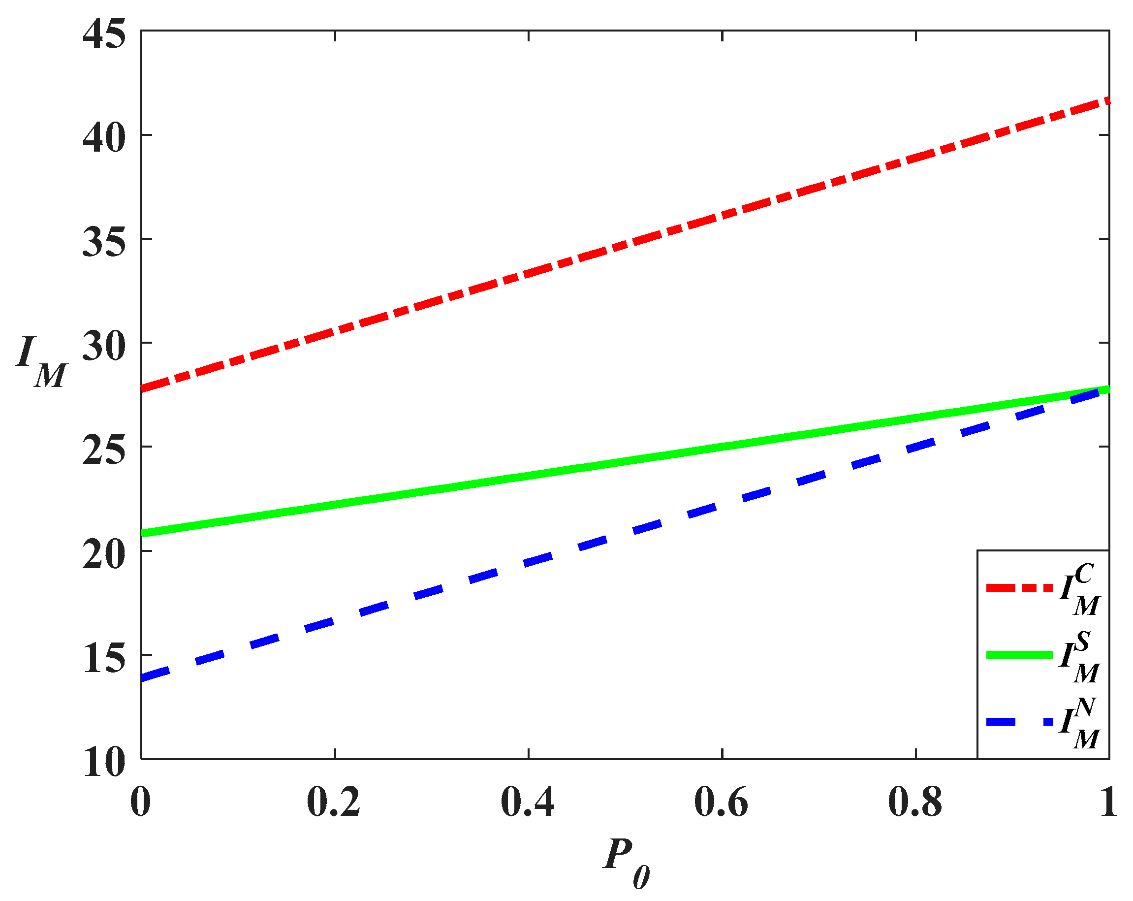
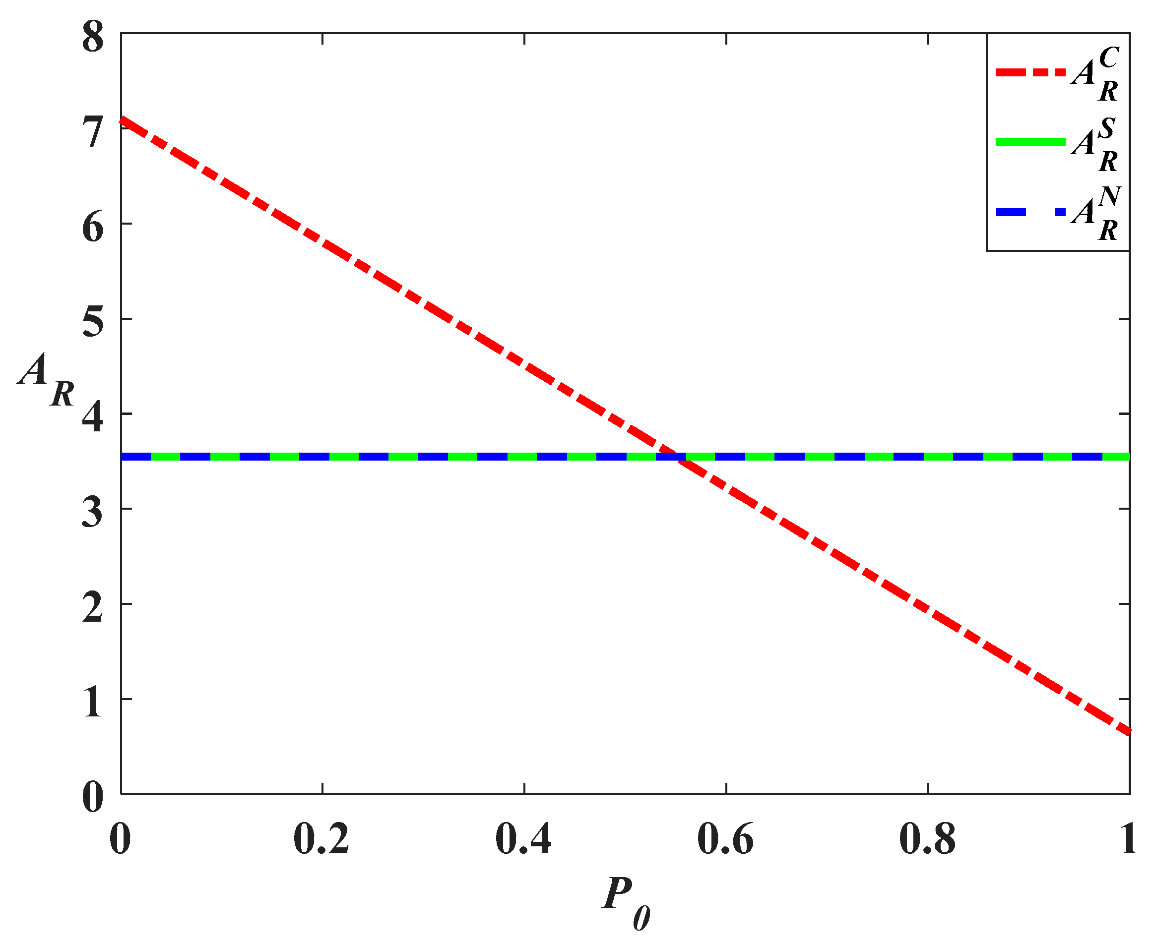
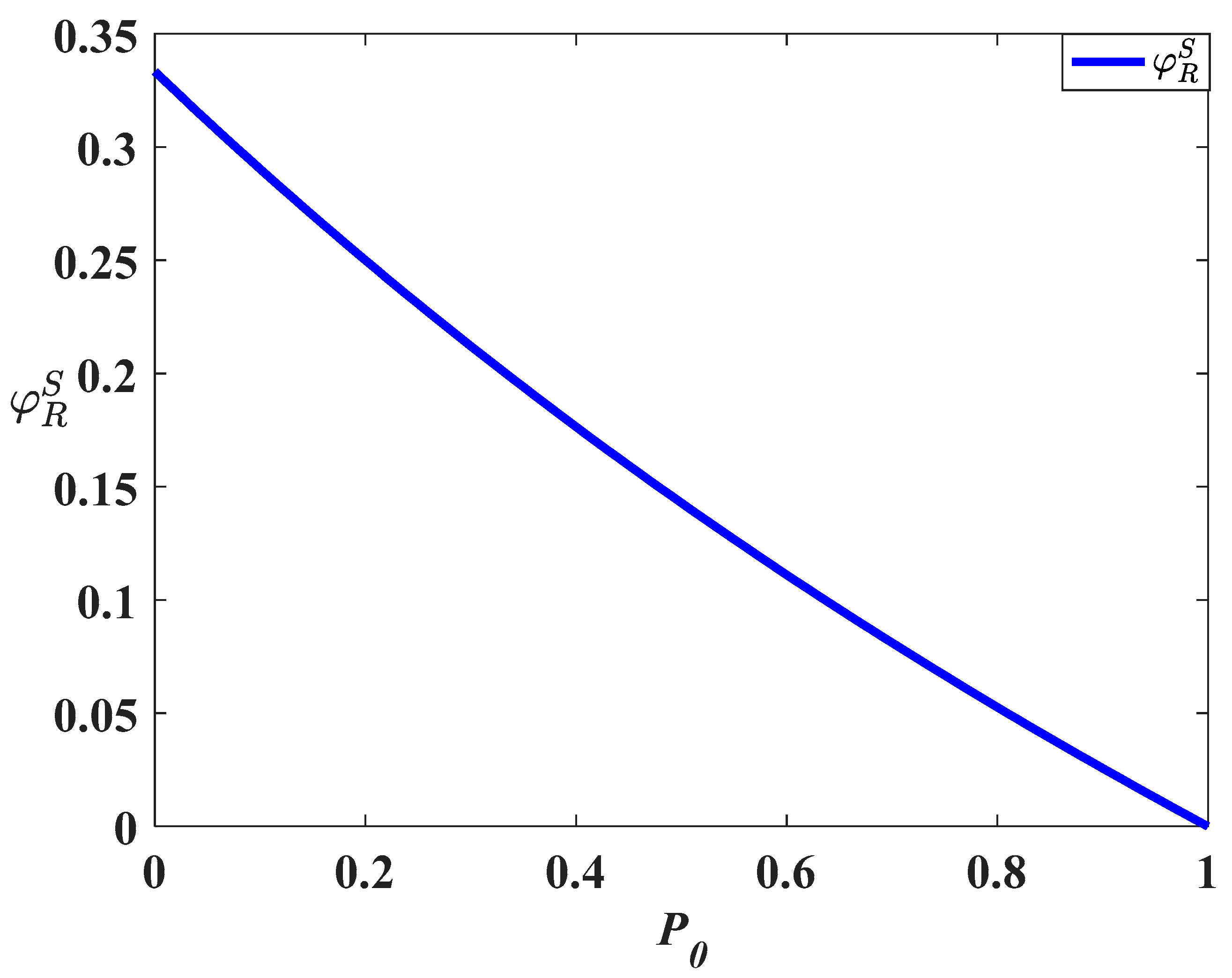
Figure 1,
Figure 2 and
Figure 3 analyze how the change in carbon trading price affects the decisions of supply chain members. According to previous analyses, to ensure that the marketing effort is positive, the trading price should satisfy
. And to make sure that the retailer will perform the cost-sharing strategy,
should satisfy
. Hence, the price
should be within the interval
.
Figure 1 shows that with the increase in carbon trading price, the manufacturer should increase their carbon reduction effort in all three scenarios. Meanwhile, the reduction effort level in the cost-sharing scenario is higher than that in the decentralized but lower than that in the centralized scenario.
Meanwhile, the growth rate of the carbon reduction level with regard to the trading price in the cost-sharing scenario is lower than that in the decentralized scenario. This is because with the increase in trading price, the retailer will reduce the cost-share ratio (as is shown in
Figure 3) and when
(
) the retailer will not undertake the carbon reduction cost and the carbon reduction level in the cost-sharing scenario is identical to that in the decentralized scenario. This result shows the fact that the increase in carbon trading price will decrease the probability of the retailer conducting the cost-sharing strategy and reduce the improving effect of the strategy.
Figure 2 shows that in the centralized scenario, with the increase in carbon trading price, the retailer should reduce their marketing effort and when
(
), the marketing effort level will even be lower than those in the other two scenarios. Meanwhile, the carbon trading price has no effect on the marketing effort levels in decentralized and cost-sharing scenarios, indicating that the increase of the price can help to reduce the carbon emission in those two scenarios.
7.1.2. The Influence of Consumer Environmental Awareness
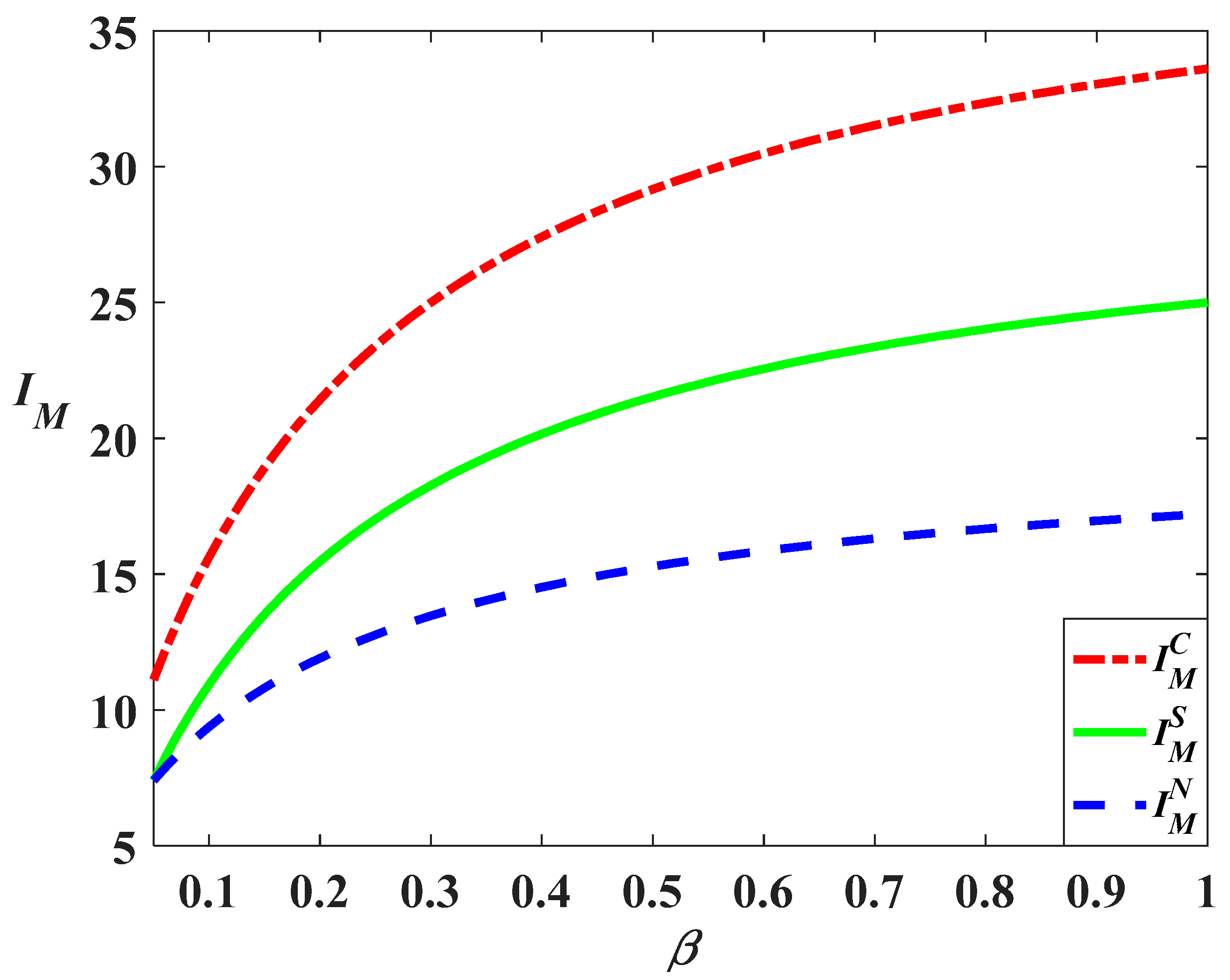
Figure 4,
Figure 5 and
Figure 6 analyze the influences of consumers’ environmental awareness on the optimal decisions of supply chain members.
Figure 4 indicates that when the consumers’ environmental awareness increases, the manufacturer should enhance the carbon reduction effort to reduce carbon emissions. Moreover, when consumers’ environmental awareness equals
(this means that we have
and
now), the carbon reduction effort in the decentralized scenario is identical to that in the cost-sharing scenario. But the carbon reduction effort in the cost-sharing scenario will become higher than that in the decentralized scenario as environmental awareness increases. This is because the retailer will increase the ratio of cost-sharing, as is shown in
Figure 6, with the increase in awareness.
Figure 5 shows that the retailer will decrease the marketing effort with the increase of environmental awareness. Hence, the increase in consumers’ environmental awareness contributes to carbon emission reduction by enhancing the carbon reduction effort and lowering the marketing effort.
7.2. Time Trajectories of Goodwill and Carbon Emission in Different Scenarios
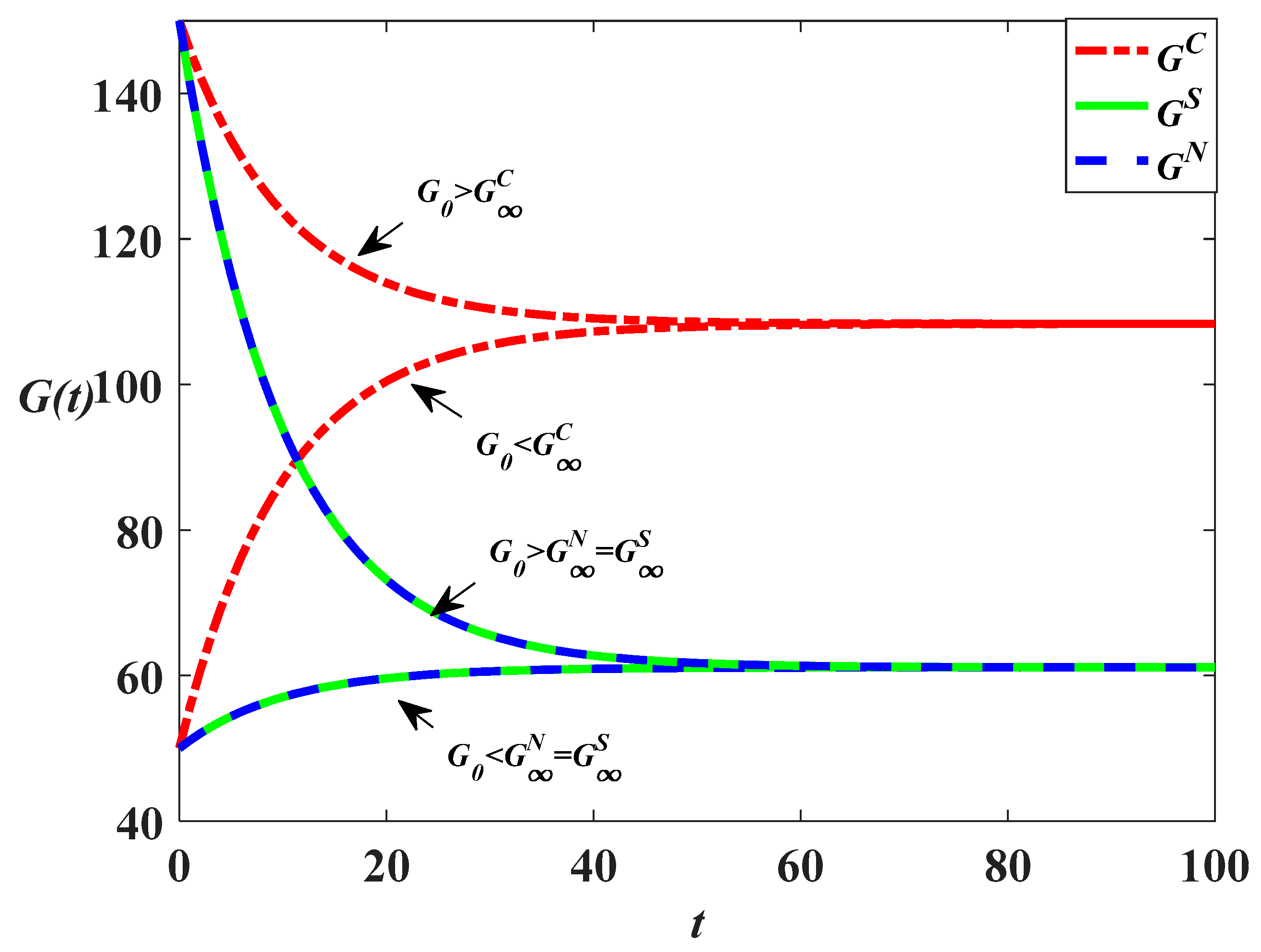
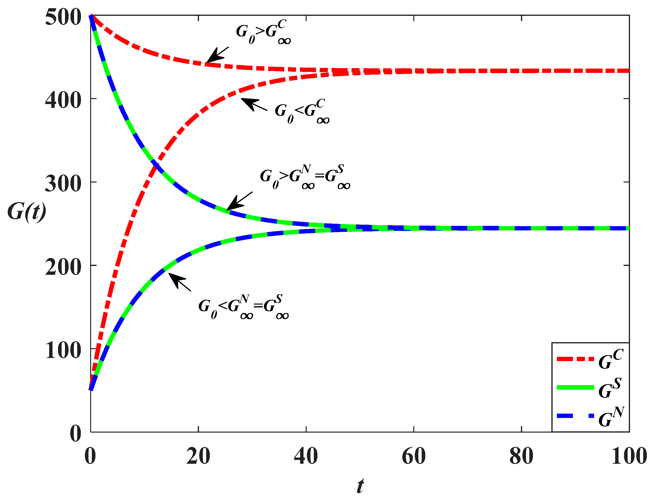
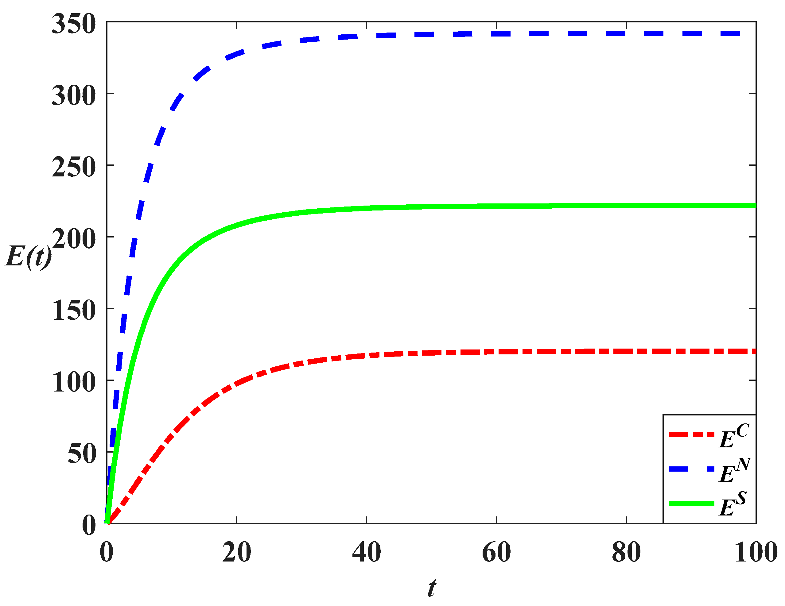
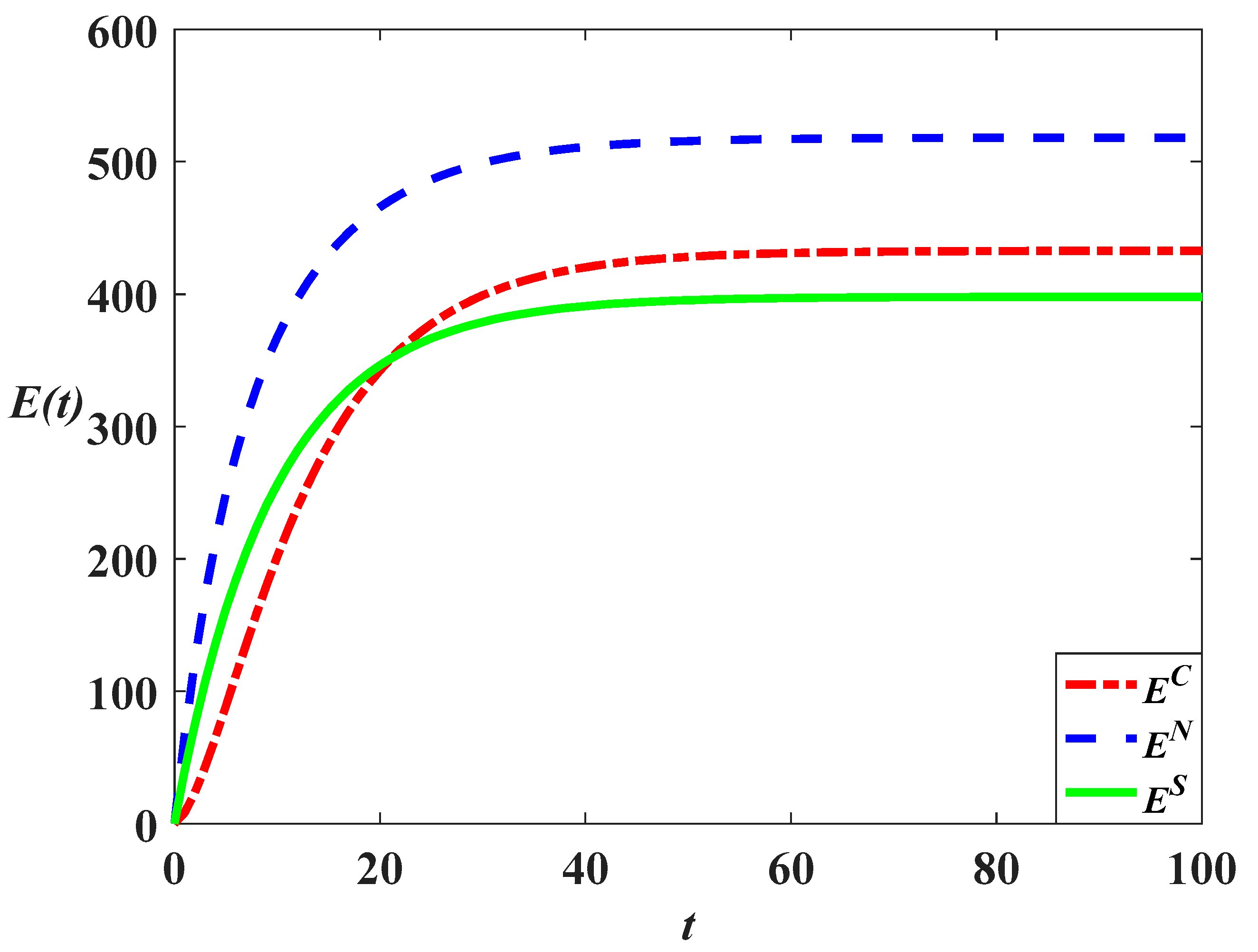
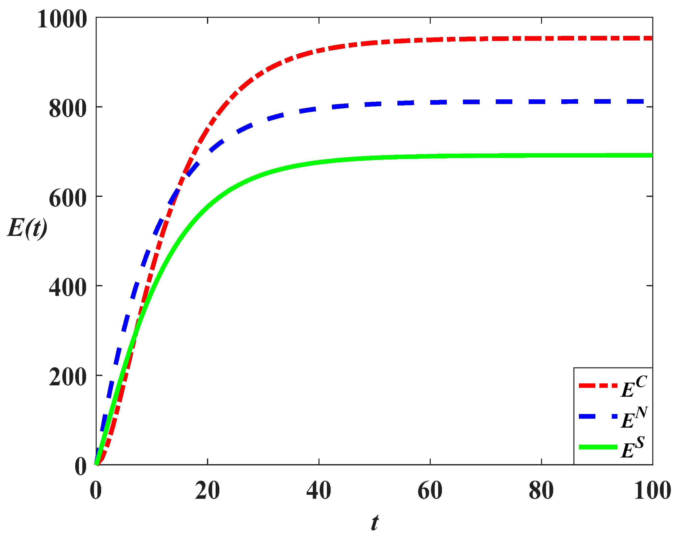
We first analyze the time trajectories of goodwill in the three scenarios (we only consider the
scenario), as shown in
Figure 7,
Figure 8 and
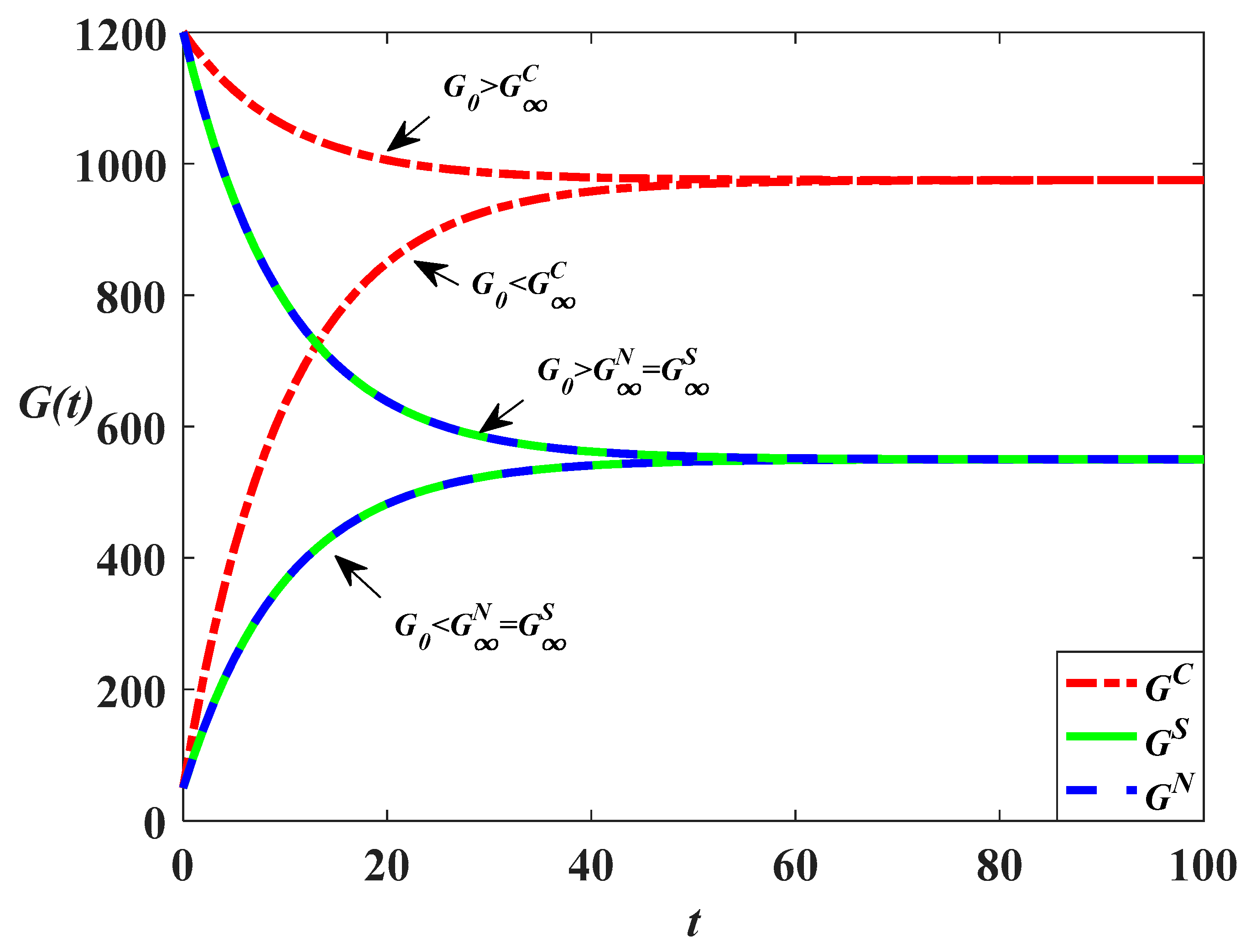
Figure 9. Since the marketing effort level in the centralized scenario is highest when the carbon trading price is relatively low, the goodwill level in this scenario is also highest. Meanwhile, since the cost-sharing strategy has no influence on the retailer’s decision, the goodwill level in the decentralized scenario will be identical to that in the cost-sharing scenario. It can also be found from
Figure 7,
Figure 8 and
Figure 9 that if the initial goodwill is high, the goodwill in the three scenarios will gradually decrease and eventually converge to a steady state. The function of the marketing effort is to prevent the goodwill from declining exponentially. But if the initial goodwill is low, the goodwill in the three scenarios will gradually increase and eventually reach a steady state. In addition, the goodwill directly increases the stock of carbon emissions and it can be learned from previous analysis that even the carbon reduction effort level in the centralized scenario is highest, the carbon emission in this scenario may not be the lowest. This is because when
, the marketing effort and goodwill level in this scenario are also highest. The carbon emissions in different scenarios are compared as follows:
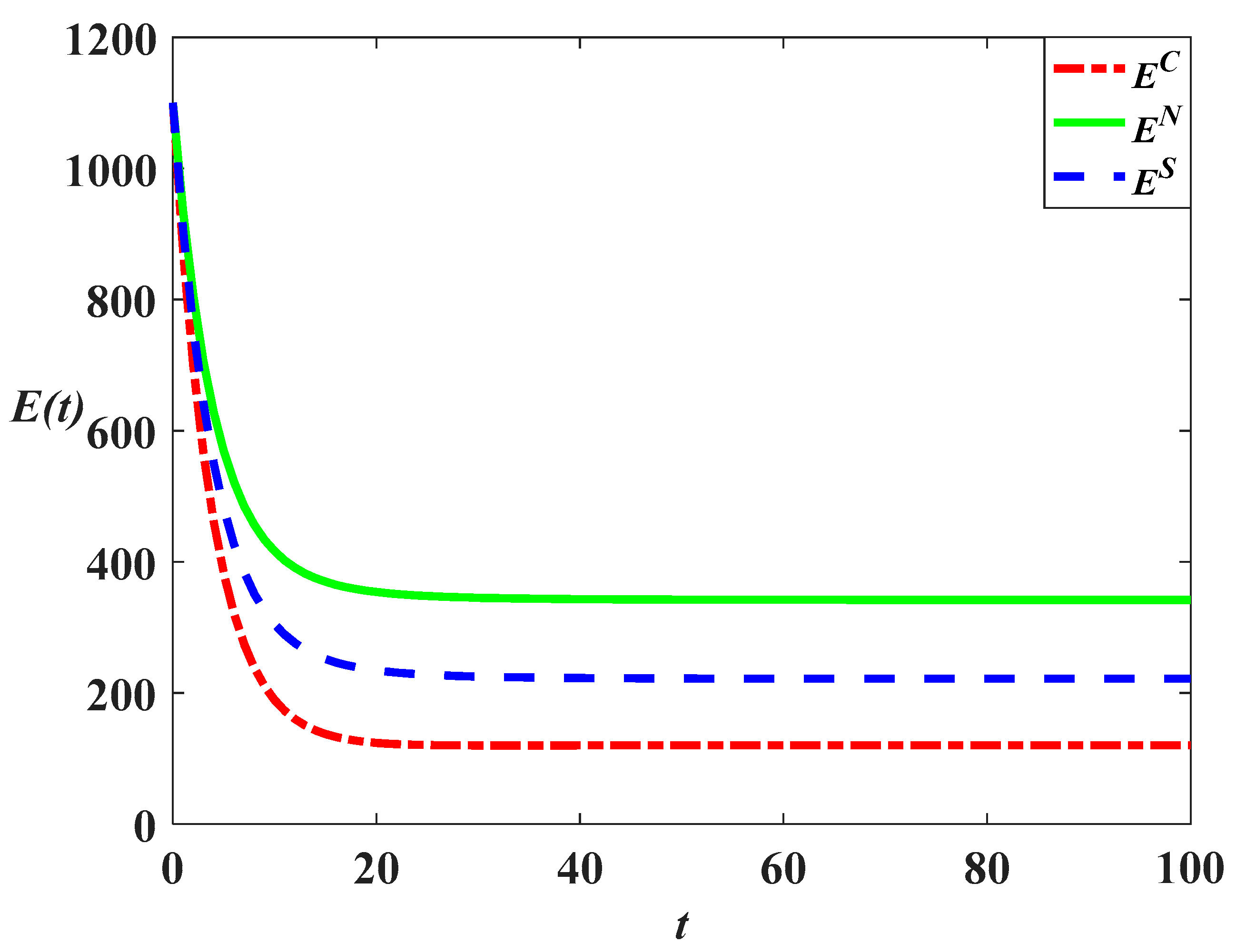
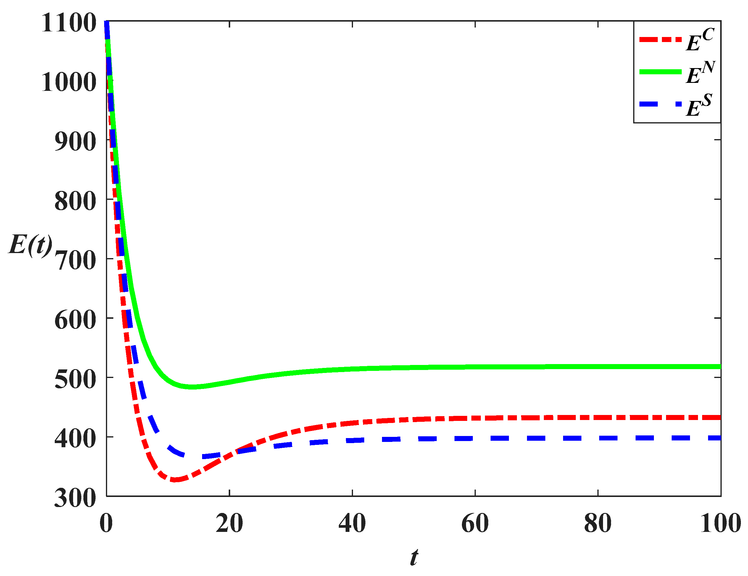
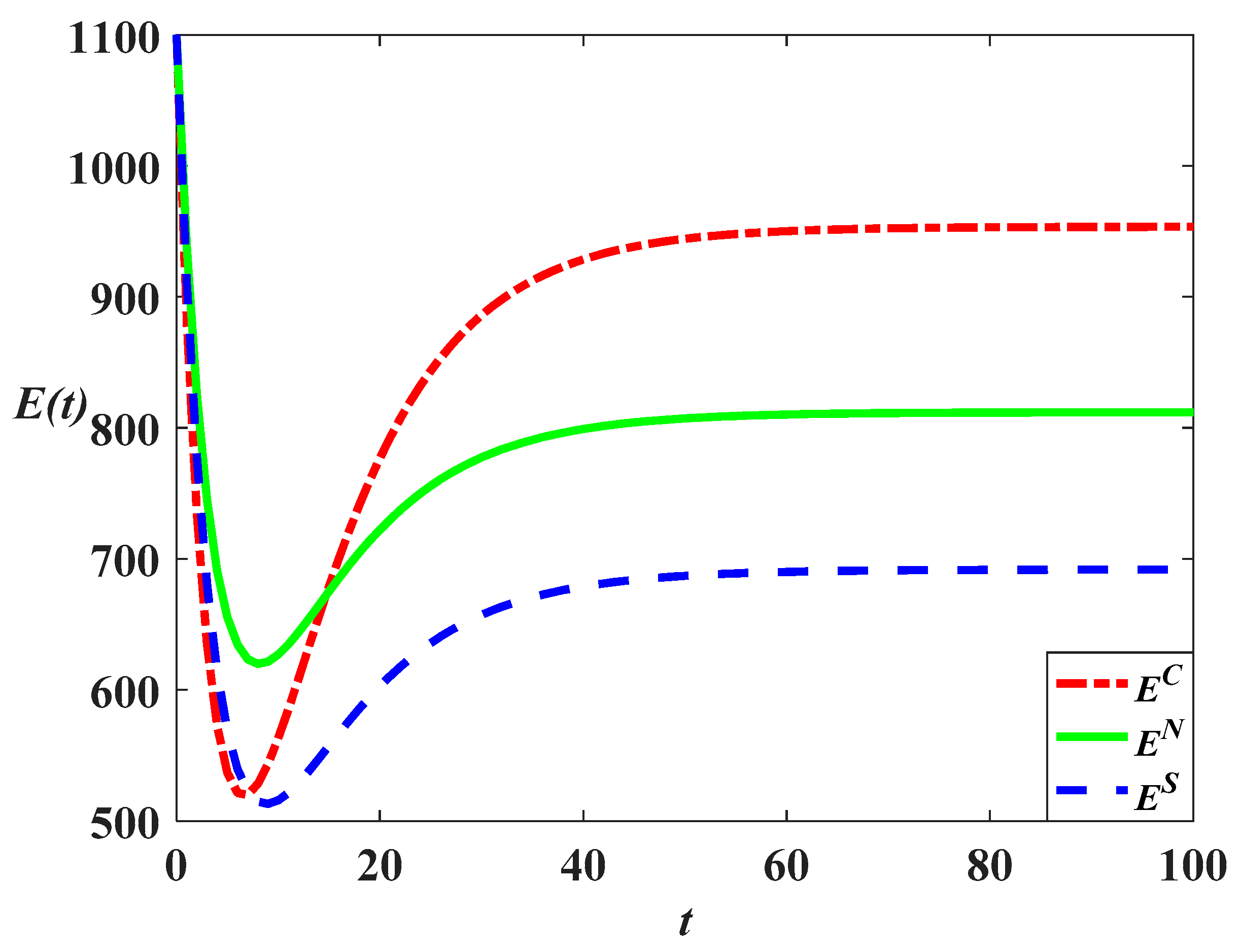
The equations above show that the carbon emission level in the cost-sharing scenario is always lower than that in the decentralized scenario, as shown in
Figure 10,
Figure 11,
Figure 12,
Figure 13,
Figure 14 and
Figure 15. This is because the cost-sharing strategy can enhance the carbon reduction effort but will not increase the marketing effort. However, the relationship between the carbon emission level in the centralized scenario and carbon emission levels in the other two scenarios are uncertain. When
, the relationship is
, indicating that the carbon emission level in the centralized scenario is the lowest of the three scenarios, as shown in
Figure 10 and
Figure 13. When
, the relationship is
, indicating that the carbon emission level in the centralized scenario is higher than that in the cost-sharing scenario, but lower than that in the decentralized scenario, as shown in
Figure 11 and
Figure 14. When
, the relationship is
, indicating that the carbon emission level in the centralized scenario is highest, as shown in
Figure 12 and
Figure 15. The comparison result mainly depends on the value of goodwill.
Figure 7,
Figure 8 and
Figure 9 depict the time trajectories of goodwill when
,
and
. It can be found from
Figure 7,
Figure 8 and
Figure 9 that with the increase of
, the difference between the steady-state value of goodwill level in the centralized scenario and those in the other two scenarios will gradually increase, indicating that when the emission reduction level remains unchanged, the influence of goodwill on carbon emission will be greater with the increase of
. Hence, from the application perspective, full cooperation may not help to reduce carbon emissions, but the cost-sharing strategy is certain to help reduce carbon emissions. When the marketing effort is very effective in enhancing goodwill (
is relatively large), the supply chain members should adopt the cost-sharing strategy to reduce carbon emissions. But if the marketing effort is less effective (
is relatively small), then complete cooperation is the most effective method of reducing the carbon emission. However, it is difficult to achieve complete cooperation in practice; we use the two-subsidy and revenue-sharing mechanism to coordinate the supply chain.
Meanwhile,
Figure 10,
Figure 11,
Figure 12,
Figure 13,
Figure 14 and
Figure 15 analyze the time trajectories of carbon emission with a different initial value.
Figure 10,
Figure 11 and
Figure 12 show that when the initial carbon emission is higher than the steady-state level, the carbon emission will first decrease due to the impact of emission reduction effort in the initial stage and then gradually increase to the steady-state value with the increase of goodwill level. When the initial carbon emission value is low, the level of goodwill will dominate the development of carbon emission until it converges to the steady-state value.
7.3. Feasibility of Coordination Strategy
This section analyzes the feasibility of the coordination strategy. We use the two-subsidy and revenue-sharing mechanism to coordinate the supply chain in
Section 5. The necessary condition of implementing this mechanism is to ensure that both supply chain members can get more profits under this mechanism than those in the decentralized scenario. Hence, it is necessary to discuss the feasible range of the sharing ratio so that both members can accept the contract. The results of the numerical analysis are shown in
Table 1.
It can be found from
Table 1 that under the coordination mechanism, the overall profit of the supply chain system is identical to that in the centralized scenario and higher than that in the decentralized scenario. But the profit of each member varies with the change in the revenue-sharing ratio. When the sharing ratio increases, the manufacturer’s profit under the mechanism will gradually decrease, and when this ratio reaches
, the manufacturer can only acquire the profit identical to that in the decentralized scenario. Hence, the upper limit of the sharing ratio is
and the manufacturer will not further increase the ratio. Meanwhile, when the sharing ratio decreases, the retailer’s profit will also decrease. If the ratio falls to
, the retailer can only acquire profit identical to that in the decentralized scenario and will refuse to accept the mechanism if the manufacturer continues to reduce the sharing ratio, indicating that the lower limit of the ratio should be
. Hence, the range of the revenue-share ratio is
, within which both supply chain members can obtain more profits than those in the decentralized scenario and total profit is as same as that in the centralized scenario. The supply chain can be fully coordinated. The upper and lower limit of the sharing ratio are calculated based on the value of parameters set at the beginning of this section. When the value of parameters changes, the limits of sharing ratio will also change accordingly. However, the numerical analysis proves that when the revenue sharing ratio falls within a certain range, the two-subsidy and revenue-sharing mechanism is able to coordinate the supply chain system.
8. Conclusions
This paper aims to study the dynamic carbon reduction and marketing decisions of supply chain members with consideration of consumers’ environmental awareness and carbon trading regulation. Hence, a differential game model is constructed and the optimal decisions and profits in the centralized, decentralized, and cost-sharing scenarios are studied, respectively. Based on the results of different scenarios, a two-subsidy and revenue-sharing mechanism is designed to coordinate the supply chain. After comparing and analyzing the results in different scenarios, it can be found that:
- (1)
When consumer environmental awareness increases, the manufacturer should enhance the carbon reduction effort and the retailer should reduce the marketing effort in all scenarios. The former finding is consistent with previous research and the later is reasonable from a practical perspective. The increase in this awareness indicates that the consumers care more about environmental protection and prefer products with less carbon emission. However, marketing activities with high intensities usually result in waste of resources, generating pollutants or stimulating production and carbon emissions, which may cause the consumers to think that the product is not eco-friendly and may practically refuse to buy the products even if the retailer plans otherwise. Hence, when the consumers are environmentally sensitive, lowering the intensity of the marketing is more advisable. Jointly affected by increased carbon reduction effort and decreased marketing effort, the carbon emission of the supply chain system will decrease with the increase in environmental awareness.
- (2)
The carbon trading price positively affects the manufacturer’s carbon reduction effort in all scenarios but exerts no influence on the retailer’s marketing effort in the decentralized and cost-sharing scenario. But in the centralized scenario, the retailer should decrease the marketing effort when the carbon trading price increases, indicating that the increase in trading price can decrease the carbon emission in all scenarios. Hence, the cap-and-trade regulation can reduce carbon emissions by affecting supply chain members’ decisions. From the perspective of the government, if the government aims to reduce the carbon emission of the supply chain system, raising the carbon trading price is an effective method. Meanwhile, raising consumers’ environmental awareness is also effective in curbing carbon emissions. For example, the government can emphasize the importance of environmental protection through mass media or display the disastrous results of jeopardizing the environment to enhance the consumers’ awareness.
- (3)
The retailer’s cost-sharing strategy can help the supply chain members to acquire more profits than those in the decentralized scenario and is able to reduce the carbon emission of the system. However, in the centralized scenario, the carbon emission of the system may not be reduced. Especially when the effectiveness coefficient of a marketing effort on goodwill is large, the carbon emission in the centralized scenario is the highest among the three scenarios. Meanwhile, the existence of carbon trading regulation will decrease the probability of the retailer implementing the cost-sharing strategy and with the increase of carbon trading price, the probability decreases.
- (4)
This paper uses the two-subsidy and revenue-sharing mechanism to coordinate the supply chain. The results of the numerical analysis show that when the revenue sharing ratio is within a certain range, both supply chain members can get higher profits than those in the decentralized scenarios, and the supply chain can be fully coordinated.
This paper sets up a differential game model to theoretically discuss the influences of consumers’ environmental awareness and cap-and-trade regulation on the operational decisions in a sustainable supply chain, based on which we also use the two-subsidy and revenue-sharing mechanism to coordinate the supply chain. The future study can include empirical analysis into the study of the consumer’s environmental awareness and the cap-and-trade regulation to make the discussion more perfect. Meanwhile, we can also pay more attention to the cap-and-trade market and consider the trading price as a decision variable and study the pricing decision in the trade market.
