Article

Geospatial Analysis with Landsat Series and Sentinel-3B OLCI Satellites to Assess Changes in Land Use and Water Quality over Time in Brazil

by
Leila Dal Moro
1,
Laércio Stolfo Maculan
1,
Dieisson Pivoto
1,
Grace Tibério Cardoso
1,
Diana Pinto
2,
Bashir Adelodun
3,4,
Brian William Bodah
1,5,6,
M. Santosh
7,8,*,
Marluse Guedes Bortoluzzi
1,
Elisiane Branco
1 and
Alcindo Neckel
1,*
1
Faculdade Meridional, IMED, Passo Fundo 99070-220, Brazil
2
Department of Civil and Environmental Engineering, Universidad de la Costa, CUC, Calle 58 # 55–66, Barranquilla 080002, Colombia
3
Department of Agricultural and Biosystems Engineering, University of Ilorin, PMB 1515, Ilorin 240103, Nigeria
4
Department of Agricultural Civil Engineering, Kyungpook National University, Daegu 41566, Korea
5
Thaines and Bodah Center for Education and Development, 840 South Meadowlark Lane, Othello, WA 99344, USA
6
Yakima Valley College, Workforce Education & Applied Baccalaureate Programs, South 16th Avenue & Nob Hill Boulevard, Yakima, WA 98902, USA
7
School of Earth Sciences and Resources, China University of Geosciences Beijing, Beijing 100083, China
8
Department of Earth Science, University of Adelaide, Adelaide, SA 5005, Australia
*
Authors to whom correspondence should be addressed.
Sustainability 2022, 14(15), 9733; https://doi.org/10.3390/su14159733
Submission received: 13 July 2022 / Revised: 3 August 2022 / Accepted: 5 August 2022 / Published: 8 August 2022

Abstract

:
Geospatial analyses have gained fundamental importance on a global scale following emphasis on sustainability. Here we geospatially analyze images from Landsat 2/5/7/8 satellites captured during 1975 to 2020 in order to determine changes in land use. Sentinel-3B OLCI (Ocean Land Color Instrument) images obtained in 2019 and 2021 were utilized to assess water resources, based on water turbidity levels (TSM_NN), suspended pollution potential (ADG_443_NN) and the presence of chlorophyll-a (CHL_NN) in order to temporally monitor the effectiveness of Brazilian legislation currently in force. This work on sustainability standards was applied to a hydrographic basin dedicated to agricultural production located in southern Brazil. Satellite images from Landsat 2/5/7/8 (1975 to 2020) and Sentinel-3B OLCI (2019 and 2021) revealed that changes in land use, vegetation cover and water in the Capinguí Dam reservoir detected high concentrations of ADG_443_NN (3830 m−1), CHL_NN (20,290 mg m−3) and TSM_NN (100 gm−3). These results can alert the population to the risks to public health and harm to hydrographic preservation, capable of covering large regions.

1. Introduction

Changes in agricultural land use in hydrographic basins on a global level have proven to be unsustainable as they cause continuous environmental degradation. Therefore, the formulation of public policies aimed at mitigating possible harmful effects on the environment has gained importance [1,2]. In an attempt to understand the processes of environmental degradation that involve changes in land use, it is of fundamental importance to monitor and control the factors related to the increase in agricultural production, aimed at the sustainability of the process and food security [3,4]. Such monitoring and control also contribute to the United Nations’ Sustainable Development Goals (SDGs) through an analysis of each territory, considering that each region has distinct peculiarities and inequalities, increasing the complexity of studies and mitigation and adaptation strategies [5,6,7].
The SDGs encompass 17 goals, 169 targets and 231 indicators, where 193 UN member countries have committed to practical actions for the success of these goals aimed at the sustainability of the planet [7,8]. In this context, they address crucial issues for humanity and the environment including food production related to food security, sustainable agriculture and responsible production and consumption [5,7,8]. Since the use of agricultural land in watershed areas to increase worldwide food production, the need for geospatial studies related to environmental preservation is increasingly justified [9].
Geospatial studies consist of tools that assist in analysis and decision making to favor local and global development [9,10,11]. These land use changes have positive or negative effects on food security [9,11]. Brazil is experiencing a negative effect in which food shortages may arise in the coming years due to population growth combined with the lack of Brazilian land available for agricultural crops. Additionally, the increase in climate vulnerability that affects our planet has begun to compromise food production through both severe droughts and heavy rains [12,13]. As mitigating factors to improve agricultural productivity and promote soil conservation, trees are planted in relation to agricultural management through a mix of different species interspersed in the same area of land [14]. Climate change and land conservation issues are part of the 17 SDGs, which require actions and initiatives to combat climate fluctuations as well as protect life on Earth [5,7,8]. These sustainability-related factors lead to positive issues in areas of agricultural cultivation. By meeting food demands in a sustainable way, we can help reduce rates of local and global intensification [15,16]. Thus, in this study, we focus on sustainability standards in relation to a hydrographic region of agricultural cultivation in southern Brazil.
Remote sensing has emerged as one of the modern technologies worldwide. It uses satellite imagery to obtain geospatial information from the Earth’s surface on a temporal scale [17,18]. Studies [19,20,21,22,23,24] involving images from Landsat 2/5/7/8 and Sentinel-3B OLCI satellites, with the purpose of accumulating terrestrial information by wavelength, allowed extremely reliable detailed information and analysis on land use and water resources on a global level, from 22 January 1975 (the year Landsat 2 was launched) to the present day. These images were combined with those produced by the Landsat 8 satellite, launched on 11 February 2013 and the Sentinel-3B OLCI, launched into space orbit on 16 February 2016. The images from the Sentinel-3B OLCI satellite allow an accurate analysis of the water quality of hydrographic basins, related to the environmental impact caused by the agricultural activities at micro and macro scales. Sentinel-3B OLCI has the capability to measure water turbidity levels (TSM_NN), suspended pollution potential (ADG_443_NN) and the presence of chlorophyll-a (CHL_NN) [24].
To measure parameters that allow for the identification of land uses, pointing out agricultural areas, water resources, forests and urbanized areas. This highlights the changes that have occurred in land use over time [19,20,21,22,23,24]. A combination of forests, food production areas and the strengthening of agroforestry systems is the best way to improve ecosystem services at the local level, and information from satellite images serves as a basis for the construction of future public policies regulating a greater production of food in addition to the utilization of environmental preservation techniques [9,25,26].
Brazilian rural development has been guided by numerous cases related to the exploitation of natural resources to expand agricultural areas since the early 19th century [27,28]. More recently however, Brazil has begun imposing legal rules requiring environmental preservation. This began with National Environmental Policy (PNMA) art. 225 of the Federal Constitution (1988), within the Environmental Crimes Law (Law n. 9.605/1998) and the Brazilian Forest Code, which together contribute to more sustainable agricultural production [29,30]. In 2012, Brazil created the Rural Environmental Registry (CAR) through Law 7830 of the National Rural Environmental Registry System (SICAR) in order to provide data to help understand Brazilian land use [31]. SICAR provides information on rural land use coverage and compliance with environmental regulations, helping agents to monitor the environmental impacts of Brazilian agriculture and forestry activities [31,32]. In this perspective, Brazil, through the creation of CAR, reinforces the commitment assumed with UN member countries to achieve the outlined SDGs by 2030; collectively seeking to carry out quality research on sustainable development aimed at land use in watersheds and related to production agriculture, thus raising food security standards on a global scale [9,33]. The use of satellite images in geospatial studies aimed at monitoring the effectiveness of historical environmental legislation has proved to be most effective in this context [31,34].
The general objective of this study is to geospatially analyze images from the Landsat 2/5/7/8 satellites obtained from 1975 to 2020 to detect changes in land use. Images obtained from the Sentinel-3B OLCI satellite from 2019 to 2021 were also analyzed to evaluate the quality of water resources based on levels of TSM_NN, ADG_443_NN and CHL_NN. This water quality analysis allowed us to monitor the effectiveness of current legislation regarding sustainability standards in a watershed focused on agricultural production located in southern Brazil. The methodologies utilized in this study are important as they relate to patterns of agricultural evolution, typical of food security reinforced by the UN, with soil use and quality of water resources in Brazil, which exports food commodities worldwide.

2. Materials and Methods

2.1. Study Area

This study examines agricultural areas in the Passo Fundo River Basin surrounding the Capinguí Dam and associated reservoir, located in the rural areas of the cities of Passo Fundo, Marau and Mato Castelhano in the Brazilian state of Rio Grande do Sul (Figure 1) [35]. The city of Passo Fundo had an estimated population of 203,275 inhabitants in 2019, with a population density of 235.9 inhabitants/km2. It encompasses a territorial area of 783,603 km2 [35]. The city of Marau had an estimated population of 44,161 inhabitants in 2019 with a population density of 56 inhabitants/km2, and comprised a territorial area of 649,770 km2. The city of Mato Castelhano had a total 2019 population of 2614 inhabitants over a territorial area of 238.4 km2 [9,35].
The Capinguí Dam was built in 1933 by the CEEE (Companhia Estadual de Energia Elétrica) in order to operate of the Capinguí Hydroelectric Power Plant. Initially constructed only for the generation of electricity, the reservoir created by the dam currently serves as a public water supply [36]. The agricultural production area studied corresponds to the rural areas located within the administrative limits of the cities of Passo Fundo, Marau and Mato Castelhano, which together surround the Capinguí Dam. In 1975, agricultural production covered an area of 111,283 m2 [9,35,36]. Agricultural production serves as the driver of the local economy. In the first quarter of 2021 alone, the state of Rio Grande do Sul produced USD 3071 worth of exports [35]. The rural production area of the cities of Passo Fundo, Marau and Mato Castelhano make up more than 10% of the total production area in Rio Grande do Sul state [9,35]. The total area examined in this study is equivalent to 111,283 m2, an area under intense inspection by environmental agencies in order to ensure compliance with Brazilian environmental legislation due to the influence of the Capinguí Dam. In this study, it was necessary to analyze the classes referring to the Landsat satellite images and the water quality with the Sentinel-3B OLCI satellite, because the studied use areas are in an area of direct influence with the waters of the Capinguí dam [9,35,36]. It is highlighted that the study area is in constant inspection, where it is possible to safely assess the effectiveness of Brazilian public policy aimed at environmental preservation and sustainability.

2.2. Methods of Data Collection

This study highlights that the pre-processing phase considered the study area, based on the Landsat satellite series made available by the United States Geological Survey (USGS), in which the Landsat satellite image series were selected from March 1975, 1985, 1992, 2001, 2011 and 2020, as they present periods of greater absence of clouds and precipitation [9,35,36]. It is highlighting the importance of maintaining geospatial analysis with similar characteristics in the landscape. In this study, the land uses were analyzed in the summer. Recalling that the USGS made available the satellite images already calibrated, Landsat 2, with a spectral resolution of 80 m, an inclination of 99.2°; Landsat 5 with a spatial resolution of 80 m and inclination of 98.20° and Landsat 7 and 8 with multispectral spatial resolutions of 30.0 m, with an inclination of 98.2° [37], constituting the general average of R2 = 0.93 for the entire studied area. These images were projected from the coordinates of WGS 84 for the Geocentric Reference System for the Americas (SIRGAS 2000) in the QGIS software (QGIS 3.10 Development Team—Brazil), in which masks of the study area, necessary for the clipping, were created, in addition to the Supervised Classification by the Dzetsaka tool. The land use maps of the study area were prepared from Landsat 2/5/7/8 satellite images (Table 1). The images were obtained from the website of the USGS [37], processed utilizing QGIS software—Geographic Information System software (GIS), version 2.18. Analyzed images were selected based on low cloud cover, thus ensuring adequate levels of visibility applied to the analyzed areas [17,19,38]. This justifies the selection of images from the Landsat satellite series only for March in relation to the analyzed period, as there are low incidences of cloud shadows.
Land use maps were created based on the following approach. Map mosaics were constructed by visualizing false colors in the Red, Green and Blue (RGB) system [39]. Different bands were utilized depending on the characteristics and specificity of the Landsat satellite [22,23,24]. This study was based on the literature [2,9,14] where it was possible to follow the land use classification stage; classes were predetermined: water resource (1), agricultural land (2), forest (3) and exposed soil (4) because they are the main elements of the landscape. The images were designed for the artificial intelligence of the Dzetsaka plugin, allowing the categories to be correctly identified, so it was necessary to increase the number of features to solve one of the difficulties of this study since the satellites used have different spatial resolutions. In this context, about 10 tests were carried out until reaching a current condition, increasing the number of features destined for supervised collection and classification (RGB543), where the Landsat satellite images presented in 1975 were a total of 301 features, 1985 were a total of 121 features, 1992 were a total of 130 features, 2001 were a total of 176 features and2020 were a total of 250 features, so it was possible to obtain more satisfactory results, with the model of supervised classification being performed, using the Dzetsaka tool of the QGIS software, adopting the Gaussian model [40]. This classification of satellite images generated two files in raster format (.tif) which were then treated with the Sieve tool in the QGIS software. This tool aims to remove raster polygons smaller than a certain size limit (in pixels) and replace them with the pixel value of the largest neighboring polygon, in addition to eliminating the fragments, joining the predominant morphological characteristics. The mosaics were then cut according to the spatial delimitation used for the study area. Finally, the files were converted into vector format files (shape) to extract quantitative data from the study site. It should be noted that the class of water resources can sometimes yield inconsistencies due to the following factors: the presence of clouds, water level in the Capinguí Dam reservoir and difference in the spatial resolution of the sensors present in the different satellites [24,39].
Subsequently, the data collected from Landsat 2/5/7/8 satellite images were subjected to landscape metrics, which consist of the use of various statistics to analyze the landscape [41,42]. To obtain the landscape metrics, the Lecos tool (Landscape Ecology Statistics) was used in the QGIS software. For Jung [43], it is possible to verify the statistics across the entire landscape, which allows for the calculation of various metrics in raster layers provided by satellite images. In this relation, the metric analysis of the landscape for this study was structured in the following procedures [44]: statistical analysis of the landscape composition and configuration, where the following were measured: land cover (LC); proportion of the landscape (PLAND); patch density (PD); higher patch index (LPI); larger patch area (GPA); and total core area (TCA). The following metrics were used, consisting of the quantification and parameterization of landscape changes in this study, following the methodological pattern pointed out by Zatelli et al. [44]: number of patches (NP); patch density (PD); average patch area (AREA_MN); median patch area (AREA_MD); total Edge (TE); edge density (ED); fractal dimension index (FRAC); mean shape index (MSI); percentage of like adjacencies (PLADJ); landscape division index (DIVISION); patch cohesion index (COHESION); effective mesh size (EM) and division index (SI).

2.3. Analysis of the Water Quality of the Capinguí Dam Reservoir

Analysis of the water quality in the reservoir created by the Capinguí Dam was carried out using images from the Sentinel-3B OLCI satellite, Water Full Resolution (WFR) provided by the European Space Agency (ESA). These images had a resolution of 300 meters, and were considered a maximum standard error 0.83 µg/mg in the analysis, adding to this study a 6.25% error, as the images were already calibrated by the ESA [45]. To perform the retrospective analysis, it was necessary to select images with a low percentage of clouds (Table 2). It was difficult to obtain satellite images of this region with sufficiently low cloud cover as the region has a humid subtropical local climate (Cfa), with constant rainfall distribution. What generated the presence of Altostratus clouds (As) with clouds in uniform and extensive layers, with dynamics of a tendency to not generate a shadow, which does not negatively influence the geospatial analysis with the use of satellite images [46]. Combined with an average annual temperature of 22 °C, the area experiences constant evaporation [46].
Image processing was performed using the Geographic Information System (GIS) software, SNAP version 8.0.4. To verify the water quality, three analyses were performed (TSM_NN, ADG_443_NN and CHL_NN). The 37 satellite collection points were positioned at the Capinguí Dam.

2.4. Statistical Analysis between Classes

The data collected by the Landsat 2/5/7/8 and Sentinel-3B OLCI satellite images were analyzed using Pearson’s correlation, aimed at verifying the relationship between the classes of data collected. The values of “r” in this method potentiate sweeps from 1 to −1, with values close to zero resulting in a null correlation; that is, there is no influence of one variable on the other [46,47]. A value close to 1 means that the increase in one variable influences the increase in another variable [47]. While a value close to −1 means that the increase in one variable influences the decrease in the other variable [47]. Regarding interpretation, the correlation from 0.00 to 0.19 is considered very weak; 0.20 to 0.39 is weak; 0.40 to 0.69 is moderate; 0.70 to 0.89 is strong and 0.90 to 1 is very strong [46,47]. The analysis was performed using the JASP software, version 0.13.1.0.
For K-means clustering, datasets collected by satellite were gathered and organized into a single database [48]. K-means clustering is an algorithm based on an optimization procedure where data vectors are reallocated between clusters with the minimization of an objective function until an optimal partition is obtained [48,49]. This generated the Silhouette index, which displays the average internal consistency of the cluster by evaluating the similarity of the data collected in the satellite images with respect to its own cluster compared to other clusters [49]. Consequently, the analysis involving satellite data correlated into clusters is one of the most utilized methods worldwide, capable of describing this difference in variation between geospatial variables [24].

3. Results and Discussion

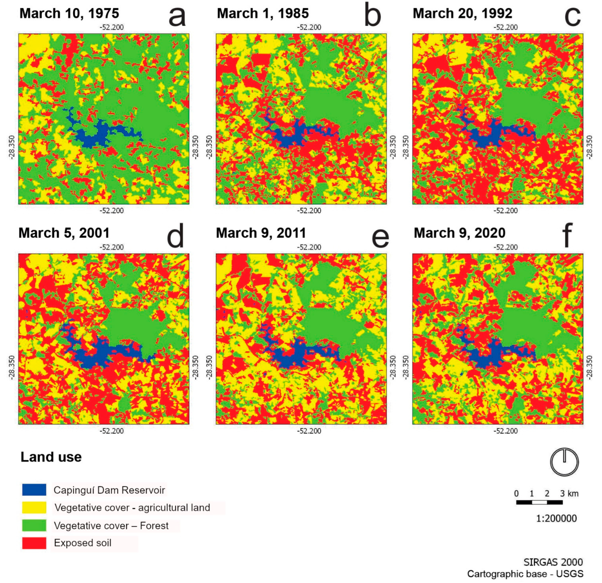
3.1. Land Use and Occupation

Images obtained from 1975 to 2020 by Landsat 2/5/7/8 satellites were analyzed for the following classes: water resources (1), agricultural land (2), forest (3) and exposed soil (4). Figure 2a shows that, in 1975, the analyzed area consisted of 57.3% of soil cover as forest, 23.9% of soil cover as agricultural area and 17.5% of the area consisted of exposed soil. Figure 2b, obtained in 1985, showed that the agricultural area had increased to 31.7%, while forest cover decreased to 31.6%. Exposed soil also increased to 28.8%. Figure 2c, obtained in 1992, agricultural area covered 23.3% of the area analyzed, forest cover consisted of 28.1% and exposed soil corresponded to 47.3% of the area. Figure 2d, obtained in 2001, yielded an agricultural area corresponding to 30.9% of the area analyzed, forest area covered 22.5% and exposed soil covered 44.8% of the analyzed area. Figure 2e, obtained in 2011, showed that 37.5% of the area was now covered by agriculture, 21.1% was forest and exposed soil covered 33.2% of the area analyzed. Figure 2f, obtained in 2020, showed an agricultural area corresponding to 31.4%, a forest area corresponding to 28.6% and exposed soil corresponding to 38.6%. The increase in exposed soil may demonstrate greater potential for leaching, with an accumulation of sediments and nutrients in water resources [23,24]. In this case, it is the Capinguí dam located in an area of direct influence [2,9,14].
It is evident that land use in this area has changed markedly since first photographed in 1975. Figure 2b displays a change in land use and occupation, with a predominance of areas destined for cultivation (agricultural land and exposed soil) as compared to the analysis of 1975.
Between 1992 and 2001, the exposed soil class was predominant, with a percentage of the area being 47.3% and 44.8%. This pattern represents a significant change when compared to other periods, which may be related to technological changes, non-agriculture and crop diversification [50,51,52]. Exposed soil could lead to erosion in production areas, contributing to socio-environmental unsustainability if effective practices aimed at recovery, conservation and soil management are not implemented [53].
As for forest cover, changes can be observed involving the loss of forest cover and gain of agricultural areas in the period from 1975 to 1985 (Figure 2). This issue may be related to the mechanization process, opening new markets for commodities, government policies and the migration of rural producers to urbanized areas [54,55]. This decrease in forested area followed a more gradual pace until 2011, showing an increase at this time. This may be related to the consolidation of environmental legislation and the evolution of technological processes that characterize Brazilian agribusiness.
The landscape underwent transformation in the years 1975, 1992, 2001 and 2020. There is a significant difference in the proportions of class in 1975 as compared to all other years; the increase in arable areas in 1985; the gradual decline of the forest surface and the predominance of exposed soil in the years 1992 and 2001. The trend line demonstrates stabilization of the transformation of the landscape for the periods of 2001, 2011 and 2020. The occurrence of temporal stabilization identified is based on the reality that, by this time, there are no more significant spaces left for deforestation in order to increase arable areas [9,56].

3.2. Analysis of Landscape Metric Composition

The analysis of the landscape composition of the study area was performed according to the following metrics: class area (CA); landscape proportion (PLAND); higher patch index (LPI) and total core area (TCA). The AC, an agropastoral area in particular, had an agricultural area corresponding to 8052 ha in 1975 and increased to 10,584 ha in 2020. Exposed soil covered an area of 5887 ha in 1975 and increased to 13,012 ha in 2020. The Forest class, in turn, had a surface of 19,263 in 1975, and had shrunk to 9632 ha by 2020. This metric is an interesting tool to vary the proportions that do not present the result of different types of land use [57].
The largest patch index (LPI) percentage is represented with more significant interconnectivity between the patches of each class [57]. The connection process between agricultural plots has been decreasing since 1975, when the index corresponded to 3.766. By 2020 it had fallen to 1.965. This factor may be related to a cultivation strategy, which seeks to optimize machinery, avoid losses and diversify cultivars, thereby enhancing sustainability in agricultural production.
The exposed soil class of the years 1992 and 2001 present an LPI of 31.8094 and 36.0303, respectively, demonstrating that there was high continuity between the patches. This phenomenon may be related to the development of herbicide-tolerant cultivars that were first implemented in Brazil in 1995, when the Brazilian Federal Government approved the Biosafety Law, which allowed the consolidation of direct seeding systems in Brazil [9]. The direct seeding system makes it possible to leave the soil less exposed, insert cover crops and, in many cases, maintain vegetative cover and vegetation throughout the year [9].
From the point of view of land use, this served as a big change in cultivation in southern Brazil. These aspects favor SDG-13, through the capture of CO2, helping increase soil bound C in an effort to fight against global climate change [8]. This vegetative cover also lessened overland flow, surface water runoff and contamination, so that SDG-6, which includes drinking water and sanitation, is also favored [8].
Total core area (TCA) consists of removing an edge area, simulating possible edge impact, and also eliminating small fragments. This metric consists of the sum of the core areas and is an important analysis for the forest class. The TCA in 1975 corresponding to an area of 111,283 m2. A gradual reduction took place until 2001, with a corresponding value of 36,325 m2, after which an increasing trend was again realized, yielding a 2011 value of 39,323 m2. The analysis of the TCA shows that a process of consolidation of the forest class in the analyzed area is underway. The 2020 measurement of 49,850 m2 shows an increase of 27.2% when compared to 2001.
Remaining forests in the study area, although showing an increase, are becoming more homogeneous. This statement can be justified by the effectiveness of Brazilian environmental legislation, mainly by measures such as the Rural Environmental Registry. This registry served as an important advance in favor of environmental preservation in Brazil, as it is a mandatory document. Landowners must provide information about the protected areas on their properties with native vegetation [29]. This factor is quite positive for the UN 2030 Agenda, where the SDGs support issues such as a diversity of life on Earth and responsible production and consumption [8,58].

3.3. Temporal Evolution of the Landscape

The statistical analysis of the configuration of the rural landscape in the study area was structured in the following metrics: number of patches (NP); patch density (PD); average patch area (AREA_MN); median patch area (AREA_MD); total edge (TE); fractal dimension index (FRAC); and edge density (ED). Thus, it is noteworthy that the number of patches (NP) is a measure that characterizes a particular class, these attributes contribute to the understanding of landscape characteristics [57]. In the forest class, it is possible to observe a process of homogenization and densification, as the number of patches decreased by 22.6% from 1992 to 2020. The forest area increased by 8% in this period. This phenomenon can be justified by the increase in mechanization that requires areas with fewer obstacles and by the consolidation of permanent preservation areas, mainly through the implementation of policies related to the Rural Environmental Registry (CAR).
As for agricultural lands and exposed soils related to agropastoral cultivation, the overall number of patches decreased until 2011, indicating the continuity of the areas. From this time, the number of spots increased, possibly indicating the appreciation of the activity and the increase in commodity prices [9]. As for the forest class, the average size of the patches is smaller when compared to the classes destined for cultivation throughout the historical series, excluding the year 1975. This question reaffirms the change in the landscape and how a significant portion of the 1975 forest class became agricultural land by 1985. It is understood that the landscape matrix is the main element that characterizes a particular landscape [59].
Edge density (ED) is edge length divided by ground cover (LC). The increase in edge perimeter was more intense in the agricultural land class and the forest class showed a decrease in edge density. This decrease, in ED, attests to the decrease in the number of small forest fragments of remaining vegetation, which confer high edge effects.
The mean shape index (MSI) refers to the ratio between the perimeter of a patch and the perimeter of the simplest patch in the same class and measures the complexity of the shape. An MSI whose value is equal to 1 demonstrates a maximum degree of compactness. If closer to zero, the MSI demonstrates how irregular the patch is [9]. The water resource class values close to 1 validate this method, as the water resources are concentrated in the reservoir created by the Capinguí Dam. The values of agricultural areas were 0.560 in 1975 and 0.579 in 2020, which indicates a certain regularity in the shape of the spots. The value for the exposed soil class, 0.367 in 1975, had fallen to 0.262 in 2020, which supports the increasing regularity and continuity necessary for agribusiness cultivation. The forest class has an MSI of 0.407 in 1975 and 0.396 in 2020. Thus, it can be said that despite the decrease in the forest surface, the patch presents low variation and continuity.
The fractal dimension index (FRAC) analysis is based on the perimeter area and quantifies the degree of complexity of the shapes. The limits of this metric range from 1, for a relatively simple patch, to 2 for patches with more complex and convoluted shapes [60]. The classes of agricultural land, exposed soil and forest have FRAC scores ranging from 1.07 to 1.11, with low variation, demonstrating the regularity of the patches over time. Despite these social and technological differences observed along the time series, it is seen that the cultivars and the forms of the beds did not change significantly over time. Over the period analyzed, technological advances and access favored agricultural productivity, which began to demand less monetary resources for production in addition to less land. In this sense, innovation, technology and infrastructure strengthened the SDGs, especially SDG 9, thus raising the degree of local sustainability.

3.4. Landscape Fragmentation

Landscape fragmentation can be analyzed using some statistical metrics such as percent of similar adjacencies (PLADJ); patch cohesion index (COHESION); effective mesh size (EM); and division index (SI). In this relationship, the degree of connectivity is measured by the PLADJ, which calculates how much similar pixels are aggregated. Values close to zero signify a level of disaggregation and values close to 1 representing greater aggregation [60]. Water resources are more aggregated, demonstrating the validity of the measurement, as the most significant spot is the Capinguí Dam reservoir. Consequently, agropastoral activities are related to agricultural land and exposed soils, which represent the highest connectivity index. The forest class corresponds to values of 0.74, which are also considered high. The landscape is characterized by homogeneity in the relationship between these two classes. The classes of exposed soils and agricultural lands were considered disaggregated in 1975. By 1985, they present aggregated values of 0.80, and 0.75 in the year 2020. The forest class in 2020 is aggregated with a PLADJ index of 0.751, which indicates a favorable level of biodiversity. Mungai et al. [61] collected data via remote sensing involving land the use needed to support future management initiatives, and aimed at the development of policies capable of guaranteeing the conservation of the environment.
Another important metric is the patch cohesion index (COHESION), which defines the ability of a species to migrate between patches and also measures the physical connection of patches in a class, where patch cohesion increases as patch type becomes more aggregated in its distribution, and more connected [60]. The classes were increasingly homogeneous in terms of cohesion and connection after 1985, with values starting at 9.8.
The split index (SI) indicates the split in a given landscape, and the index is lower when the patches are separated and of smaller dimensions [62,63]. SI reaches its maximum value when the landscape is less subdivided and the patches are closer [62,63]. That forest class was in the process of splitting. Since 2011, this process has changed as the SI has decreased. Regarding the class of agricultural land, the division increased until 1992, after which point the SI began to decrease, indicating a tendency of agglomeration between the patches. This also indicates greater homogeneity and consolidation of agricultural lands. Remembering that remote sensing at different scales reveals useful data for future research involving the mapping of land use, thus making it possible to follow the evolution of the landscape [64].

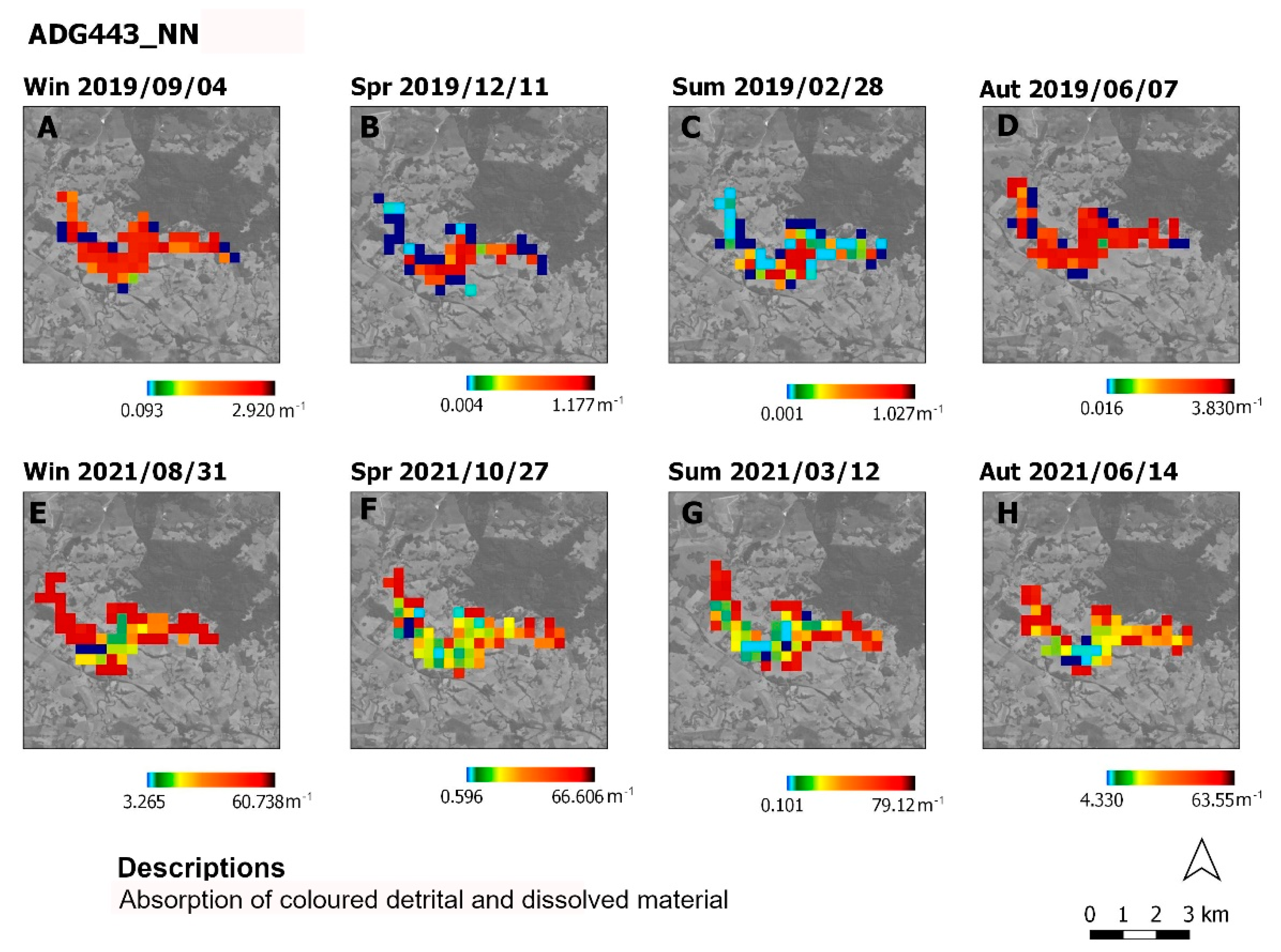
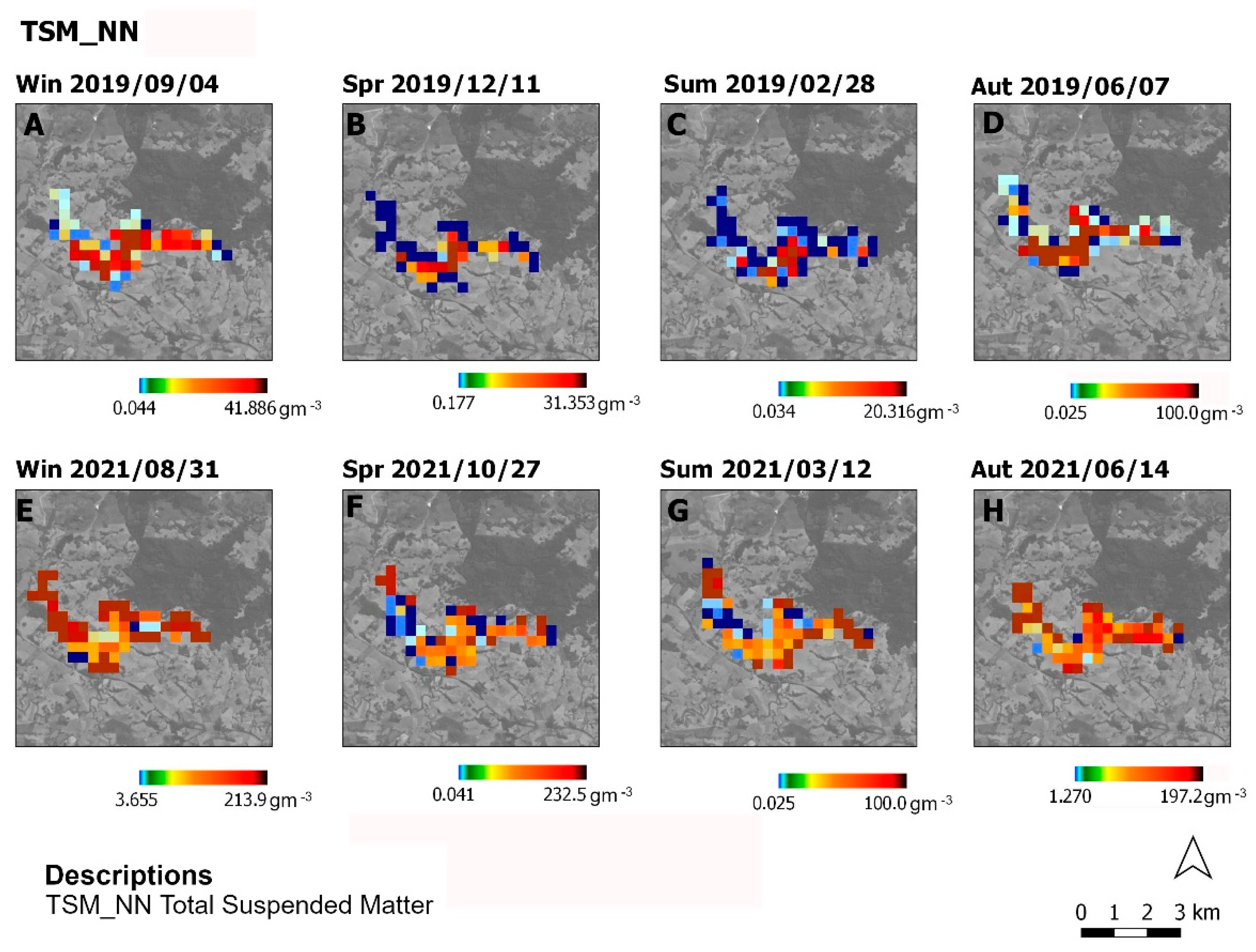
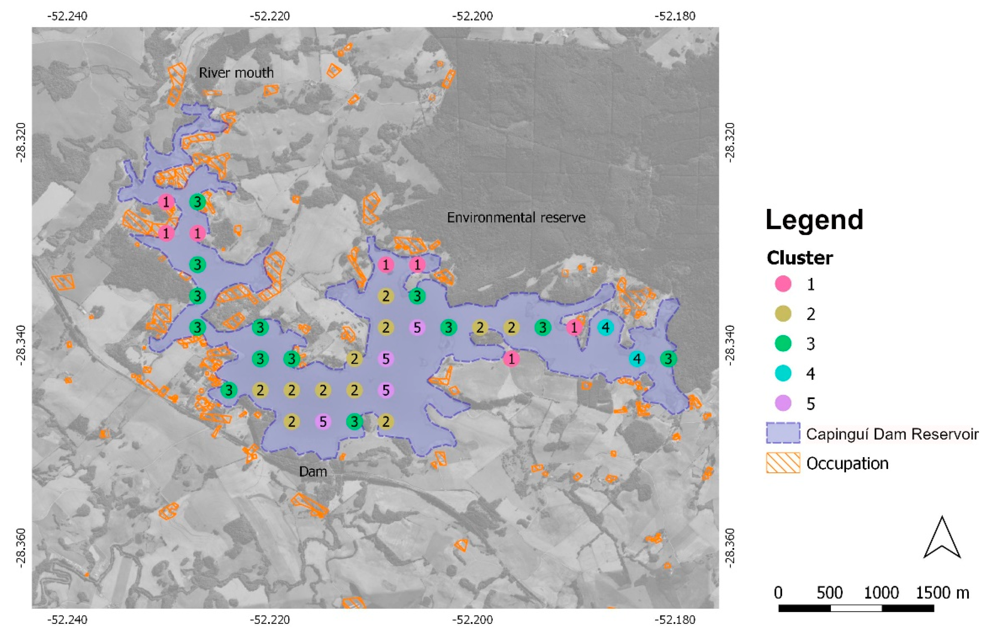
3.5. Geospatial Analysis of Water Quality

The compositions of the Sentinel-3B OLCI images were analyzed due to the importance of the Capinguí Dam for the study region. Local data, such as average rainfall per season, were also considered and are as follows: summer 2019, 160.3 mm; autumn 2019, 158.8 mm; winter 2019, 68.6 mm; spring 2019, 169.4 mm; summer 2021, 138.4 mm; autumn 2021, 106.7 mm; winter 2021, 99.16 mm; spring 2021, 139.7 mm [35]. Figure 3 demonstrates the composite Sentinel-3B OLCI images for ADG443_NN. In 2019 (Figure 3D), the autumn season had the highest concentration of suspended material on the water surface with a value of 3830 m−1, followed by winter, with a value of 2920 m−1. The values of suspended material on the water surface for the year 2021 are very high, showing that the water quality underwent a process of degradation in this period, demonstrating a possible negative influence of agricultural production on the water quality of the Capinguí Dam reservoir. The use of remote sensing becomes of fundamental importance in the evaluation of metric patterns of the landscape, capable of measuring the characteristics of the water in the geospatial perspective [65].
Figure 4 displays the composition of the Sentinel-3B OLCI images focused on CHL_NN concentrations. In the period analyzed in 2019 (Figure 4D), the autumn season had the highest concentration of chlorophyll-a concentrations with a value of 20.290 (mg (CHL_NN) m−3), followed by winter (Figure 4A), with a value of 18.290 (mg (CHL_NN) m−3). Chlorophyll-a concentrations for the year 2021 decreased in all seasons, which means lower concentrations of chlorophyll in the water, and consequently, less phytoplankton. The summer season (Figure 4C,G) has the lowest chlorophyll values, which can be explained by the characteristically dry summers in the study area.
Figure 5 shows the composites of Sentinel-3B OLCI images for TMS_NN. In the analyzed period of 2019 (Figure 5D), the autumn season had the highest concentration of water turbidity with a corresponding value of 100 gm−3. Water turbidity for the year 2021 increased in all seasons of the year. This signifies a high occurrence of environmental degradation of the water in the reservoir of the Capinguí Dam. Reducing pollution of water resources requires the implementation of environmental projects that ensure the mitigation of polluting sources that compromise their water quality [24].
Through the analysis of the data extracted from the Sentinel-3B OLCI satellite images, the K-means analysis adjusts to K = 5 (5 Clusters) for a data set that consists of a total of 37 collection points, where the value of R2 was 0.564, demonstrating that the model presents a good answer to the research question. In this relationship, the silhouette index for k = 5 clusters was 0.23, demonstrating that there is a low tendency to cluster the clusters, demonstrating that the water has high quality variability along the reservoir.
Clusters 1, 2 and 5 were influenced by the similarities found in water turbidity (TSM_NN) and surface dissolved material (ADG443_NN). Cluster 1 was influenced by the summer and spring seasons. These points can be influenced by the rainfall regime, which is low in spring and very low in summer. The indices of suspended material and water turbidity can be higher especially at the water’s edge with higher rates of urbanization. Cluster 2 was influenced by the winter season, the rainy season and the rise in the water level of the rivers. During this time, it is normal to record a higher concentration of water turbidity (TSM_NN) and surface dissolved ADG material (ADG443_NN) in the waters of the reservoir created by the Capinguí Dam. Cluster 3 presents greater diversity among the variables. What differentiates this cluster from the others is the role that Chlorophyll-a presents in all seasons of the year. The presence of chlorophyll is due to the existence of phytoplankton, these microorganisms are observed in places where there is a significant concentration of organic matter. The points that make up Cluster 3 are more prone to urban densification that is underway in the study area. According to Hou et al. [66], changes in the landscape originate from the reflection of human activities on the environment.
Figure 6 demonstrates the cluster results using georeferenced data at the 37 points surrounding the Capinguí Dam. Cluster 1 and 3 are more related to areas where occupation is more intense, Cluster 2 and 5 are more related to zones further away from the edge. The results generated from the Sentinel-3B OLCI satellite images make it possible to rethink actions of new public policies aimed at the sustainability of water resources, in addition to being one of the most modern techniques available for water quality analysis by analyzing wavelength optics made available by the ESA [24,67].

4. Conclusions

The changes that have taken place in land use in the study area have led to an increase in agricultural production in order to achieve the goals of the UN Sustainable Development Goals (SDGs), specifically the goals that address issues of food availability. This yielded an increase in the area under cultivation from 1975 to 2020. This study demonstrates that Landsat 2/5/7/8 satellites are efficient for land use analysis. For future studies in the region, the use of the Random Forest model is suggested for satellite analysis, as it presents a robust classification method, which can be compared with the data obtained in this study, using the Gaussian model analysis method.
The analyses carried out using Sentinel-3B OLCI satellite images from 2019 to 2021, aimed at assessing water resources, showed high concentrations of suspended material on the water surface (3830 m−1), chlorophyll-a (20,290 mg CHL_NN m−3) and water turbidity (100 (gm−3)). The authors suggest continued study of the water quality in the reservoir created by the Capinguí Dam in order to identify point source and non-point source sources of pollution in order to author and enforce public policies that guarantee the preservation of this water resource for future generations.
The methodology utilized in this study, which identified the effectiveness of Brazilian public policies in increasing the agricultural production system, linked to environmental preservation, can be used on a global scale in order to assess the levels of local sustainability. It can be utilized on a temporal scale through geospatial analysis in other countries of the world, considering the classification of land use on the effectiveness of public policies for environmental preservation.

Author Contributions

Conceptualization, L.D.M., E.B., D.P. (Dieisson Pivoto) and D.P. (Diana Pinto); data curation, L.S.M.; formal analysis, A.N. and B.A.; funding acquisition, B.W.B. and E.B.; investigation, L.D.M.; project administration, D.P. (Dieisson Pivoto) and D.P. (Diana Pinto); supervision, L.D.M.; visualization, A.N. and M.G.B.; writing—original draft preparation, A.N. and M.S.; writing—review and editing, G.T.C. and M.S. All authors have read and agreed to the published version of the manuscript.

Funding

This research received no external funding.

Institutional Review Board Statement

Not applicable.

Informed Consent Statement

Informed consent was obtained from all subjects involved in the study.

Data Availability Statement

Not applicable.

Acknowledgments

The authors are grateful to the European Space Agency (ESA) and the U.S. National Aeronautics and Space Administration (NASA) for providing the unpublished and treated Sentinel-3B OLCI satellite images. We also wish to thank the Center for Studies and Research on Urban Mobility (NEPMOUR/IMED) in addition to the Brazilian National Council for Scientific and Technological Development (CNPq).

Conflicts of Interest

The authors declare no conflict of interest.

References

  1. Yiran, G.A.B.; Ablo, A.D.; Asem, F.E. Urbanisation and domestic energy trends: Analysis of household energy consumption patterns in relation to land-use change in peri-urban Accra, Ghana. Land Use Policy 2020, 99, 105047. [Google Scholar] [CrossRef]
  2. Chowdhury, S.; Khan, S.; Sarker, M.F.H.; Islam, M.K.; Tamal, M.A.; Khan, N.A. Does Agricultural Ecology Cause Environmental Degradation? Empirical Evidence from Bangladesh. Heliyon 2022, 8, e09750. [Google Scholar] [CrossRef] [PubMed]
  3. Viana, C.M.; Freire, D.; Abrantes, P.; Rocha, J.; Pereira, P. Agricultural land systems importance for supporting food security and sustainable development goals: A systematic review. Sci. Total Environ. 2022, 806, 150718. [Google Scholar] [CrossRef]
  4. Parven, A.; Pal, I.; Witayangkurn, A.; Pramanik, M.; Nagai, M.; Miyazaki, H.; Wuthisakkaroon, C. Impacts of disaster and land-use change on food security and adaptation: Evidence from the delta community in Bangladesh. Int. J. Disaster Risk Reduct. 2022, 78, 103119. [Google Scholar] [CrossRef]
  5. Acuti, D.; Bellucci, M.; Manetti, G. Company disclosures concerning the resilience of cities from the Sustainable Development Goals (SDGs) perspective. Cities 2020, 99, 102608. [Google Scholar] [CrossRef]
  6. Lu, X.; Zhang, Y.; Lin, C.; Wu, F. Analysis and comprehensive evaluation of sustainable land use in China: Based on sustainable development goals framework. J. Clean. Prod. 2021, 310, 127205. [Google Scholar] [CrossRef]
  7. Dwivedi, P.P.; Sharma, D.K. Application of Shannon Entropy and COCOSO techniques to analyze performance of sustainable development goals: The case of the Indian Union Territories. Results Eng. 2022, 14, 100416. [Google Scholar] [CrossRef]
  8. United Nations. Transforming our World: The 2030 Agenda for Sustainable Development. 2015. Available online: https://sustainabledevelopment.un.org/post2015/transformingourworld/publication (accessed on 28 April 2022).
  9. Dal Moro, L.; Maculan, L.S.; Neckel, A.; Mores, G.de.V.; Pivoto, D.; Bodah, E.T.; Bodah, B.W.; Oliveira, M.L. Geotechnologies applied to the analysis of buildings involved in the production of poultry and swine to the integrated food safety system and environment. J. Environ. Chem. Eng. 2021, 9, 106475. [Google Scholar] [CrossRef]
  10. Hagos, Y.G.; Andualem, T.G. Geospatial and multi-criteria decision approach of groundwater potential zone identification in Cuma sub-basin, Southern Ethiopia. Heliyon 2021, 7, e07963. [Google Scholar] [CrossRef]
  11. Andrieu, N.; Dumas, P.; Hemmerlé, E.; Caforio, F.; Falconnier, G.N.; Blanchard, M.; Vayssières, J. Ex ante mapping of favorable zones for uptake of climate-smart agricultural practices: A case study in West Africa. Environ. Dev. 2021, 37, 100566. [Google Scholar] [CrossRef]
  12. Laufenberg, J.S.; Johnson, H.E.; Doherty, P.F.; Breck, S.W. Compounding effects of human development and a natural food shortage on a black bear population along a human development-wildland interface. Biol. Conserv. 2018, 224, 188–198. [Google Scholar] [CrossRef]
  13. Bernard, B.M.; Song, Y.; Hena, S.; Ahmad, F.; Wang, X. Assessing Africa’s Agricultural TFP for Food Security and Effects on Human Development: Evidence from 35 Countries. Sustainability 2022, 14, 6411. [Google Scholar] [CrossRef]
  14. Schürmann, A.; Kleemann, J.; Fürst, C.; Teucher, M. Assessing the relationship between land tenure issues and land cover changes around the Arabuko Sokoke Forest in Kenya. Land Use Policy 2020, 95, 104625. [Google Scholar] [CrossRef]
  15. Chen, Y.; Lu, C. A Comparative Analysis on Food Security in Bangladesh, India and Myanmar. Sustainability 2018, 10, 405. [Google Scholar] [CrossRef] [Green Version]
  16. Laborde, J.P.; Wortmann, C.S.; Blanco-Canqui, H.; Baigorria, G.A.; Lindquist, J.L. Identifying the drivers and predicting the outcome of conservation agriculture globally. Agric. Syst. 2020, 177, 102692. [Google Scholar] [CrossRef]
  17. Bodah, B.W.; Neckel, A.; Maculan, L.S.; Milanes, C.B.; Korcelski, C.; Ramírez, O.; Mendez-Espinosa, J.F.; Bodah, E.T.; Oliveira, M.L. Sentinel-5P TROPOMI satellite application for NO2 and CO studies aiming at environmental valuation. J. Clean. Prod. 2022, 357, 131960. [Google Scholar] [CrossRef]
  18. Marcinko, C.L.; Samanta, S.; Basu, O.; Harfoot, A.; Hornby, D.D.; Hutton, C.W.; Pal, S.; Watmough, G.R. Earth observation and geospatial data can predict the relative distribution of village level poverty in the Sundarban Biosphere Reserve, India. J. Environ. Manag. 2022, 313, 114950. [Google Scholar] [CrossRef]
  19. Acharki, S. PlanetScope contributions compared to Sentinel-2, and Landsat-8 for LULC mapping. Remote Sens. Appl. Soc. Environ. 2022, 27, 100774. [Google Scholar] [CrossRef]
  20. Song, D.X.; Wang, Z.; He, T.; Wang, H.; Liang, S. Estimation and validation of 30 m fractional vegetation cover over China through integrated use of Landsat 8 and Gaofen 2 data. Sci. Remote Sens. 2022, 6, 100058. [Google Scholar] [CrossRef]
  21. Shang, R.; Zhu, Z.; Zhang, J.; Qiu, S.; Yang, Z.; Li, T.; Yang, X. Near-real-time monitoring of land disturbance with harmonized Landsats 7–8 and Sentinel-2 data. Remote Sens. Environ. 2022, 278, 113073. [Google Scholar] [CrossRef]
  22. Zhang, X.; Xiao, X.; Qiu, S.; Xu, X.; Wang, X.; Chang, Q.; Wu, J.; Li, B. Quantifying latitudinal variation in land surface phenology of Spartina alterniflora saltmarshes across coastal wetlands in China by Landsat 7/8 and Sentinel-2 images. Remote Sens. Environ. 2022, 269, 112810. [Google Scholar] [CrossRef]
  23. Song, X.P.; Huang, W.; Hansen, M.C.; Potapov, P. An evaluation of Landsat, Sentinel-2, Sentinel-1 and MODIS data for crop type mapping. Sci. Remote Sens. 2021, 3, 100018. [Google Scholar] [CrossRef]
  24. Neckel, A.; Oliveira, M.L.S.; Bolaño, L.J.C.; Maculan, L.S.; dal Moro, L.; Bodah, E.T.; Moreno-Ríos, A.L.; Bodah, B.W.; Silva, L.F.O. Biophysical matter in a marine estuary identified by the Sentinel-3B OLCI satellite and the presence of terrestrial iron (Fe) nanoparticles. Mar. Pollut. Bull. 2021, 173, 112925. [Google Scholar] [CrossRef] [PubMed]
  25. Kusi, K.K.; Khattabi, A.; Mhammdi, N.; Lahssini, S. Prospective evaluation of the impact of land use change on ecosystem services in the Ourika watershed, Morocco. Land Use Policy 2020, 97, 104796. [Google Scholar] [CrossRef]
  26. Oduro Appiah, J.; Agyemang-Duah, W.; Sobeng, A.K.; Kpienbaareh, D. Analysing patterns of forest cover change and related land uses in the Tano-Offin forest reserve in Ghana: Implications for forest policy and land management. Trees For. People 2021, 5, 100105. [Google Scholar] [CrossRef]
  27. Sauer, S. Soy expansion into the agricultural frontiers of the Brazilian Amazon: The agribusiness economy and its social and environmental conflicts. Land Use Policy 2018, 79, 326–338. [Google Scholar] [CrossRef]
  28. Bin, D. Agricultural dispossessions during the 1964–1985 Brazilian dictatorship. Political Geogr. 2021, 84, 102307. [Google Scholar] [CrossRef]
  29. Roitman, I.; Vieira, L.C.G.; Jacobson, T.K.B.; Bustamante, M.M.da.C.; Silva Marcondes, N.J.; Cury, K.; Silva Estevam, L.; Ribeiro, R.J.da.C.; Ribeiro, V.; Stabile, M.C.; et al. Rural Environmental Registry: An innovative model for land-use and environmental policies. Land Use Policy 2018, 76, 95–102. [Google Scholar] [CrossRef]
  30. Preto, M.D.F.; Garcia, A.S.; Nakai, R.S.; Casarin, L.P.; Vilela, V.M.D.F.N.; Ballester, M.V.R. The role of environmental legislation and land use patterns on riparian deforestation dynamics in an Amazonian agricultural frontier (MT, Brazil). Land Use Policy 2022, 118, 106132. [Google Scholar] [CrossRef]
  31. Moraes, L.A.F.de.; Floreano, I.X. LULC zoning in the “Madeira river” settlement, legal Amazon, Brazil, before and after implementation of the rural environmental registry (CAR) (2008–2018). Environ. Dev. 2022, 43, 100725. [Google Scholar] [CrossRef]
  32. Arvor, D.; Silgueiro, V.; Manzon Nunes, G.; Nabucet, J.; Pereira Dias, A. The 2008 map of consolidated rural areas in the Brazilian Legal Amazon state of Mato Grosso: Accuracy assessment and implications for the environmental regularization of rural properties. Land Use Policy 2021, 103, 105281. [Google Scholar] [CrossRef]
  33. Leal Filho, W.; Azeiteiro, U.; Alves, F.; Pace, P.; Mifsud, M.; Brandli, L.L.; Caeiro, S.S.; Disterheft, A. Reinvigorating the sustainable development research agenda: The role of the sustainable development goals (SDG). Int. J. Sustain. Dev. World Ecol. 2017, 25, 131–142. [Google Scholar] [CrossRef] [Green Version]
  34. Coelho Junior, M.G.; Biju, B.P.; Silva Neto, E.C.D.; Oliveira, A.L.D.; Tavares, A.A.D.O.; Basso, V.M.; Turetta, A.P.D.; Carvalho, A.G.D.; Sansevero, J.B.B. Improving the management effectiveness and decision-making by stakeholders’ perspectives: A case study in a protected area from the Brazilian Atlantic Forest. J. Environ. Manag. 2020, 272, 111083. [Google Scholar] [CrossRef]
  35. IBGE. Brazilian Institute of Geography and Statistics, Demographic Data of 2022—Brazil. 2022. Available online: https://cidades.ibge.gov.br/brasil/rs/passo-fundo/panorama (accessed on 10 March 2022).
  36. Zafar, M.; Tiecher, T.; Capoane, V.; Troian, A.; dos Santos, D.R. Characteristics, lability and distribution of phosphorus in suspended sediment from a subtropical catchment under diverse anthropic pressure in Southern Brazil. Ecol. Eng. 2017, 100, 28–45. [Google Scholar] [CrossRef]
  37. USGS. Global Visualization Viewer. 2022. Available online: https://glovis.usgs.gov (accessed on 1 March 2022).
  38. Wang, J.; Yang, D.; Chen, S.; Zhu, X.; Wu, S.; Bogonovich, M.; Guo, Z.; Zhu, Z.; Wu, J. Automatic cloud and cloud shadow detection in tropical areas for PlanetScope satellite images. Remote Sens. Environ. 2021, 264, 112604. [Google Scholar] [CrossRef]
  39. Qingyun, F.; Zhaokui, W. Cross-modality attentive feature fusion for object detection in multispectral remote sensing imagery. Pattern Recognit. 2022, 130, 108786. [Google Scholar] [CrossRef]
  40. Fauvel, M.; Dechesne, C.; Zullo, A.; Ferraty, F. Fast Forward Feature Selection of Hyperspectral Images for Classification With Gaussian Mixture Models. IEEE J. Sel. Top. Appl. Earth Obs. Remote Sens. 2015, 8, 2824–2831. [Google Scholar] [CrossRef]
  41. Zhang, Y.; Balzter, H.; Zou, C.; Xu, H.; Tang, F. Characterizing bi-temporal patterns of land surface temperature using landscape metrics based on sub-pixel classifications from Landsat TM/ETM+. Int. J. Appl. Earth Obs. Geoinf. 2015, 42, 87–96. [Google Scholar] [CrossRef] [Green Version]
  42. Abalo, M.; Badabate, D.; Fousseni, F.; Kpérkouma, W.; Koffi, A. Landscape-based analysis of wetlands patterns in the Ogou River basin in Togo (West Africa). Environ. Chall. 2021, 2, 100013. [Google Scholar] [CrossRef]
  43. Jung, M. LecoS—A python plugin for automated landscape ecology analysis. Ecol. Inform. 2016, 31, 18–21. [Google Scholar] [CrossRef]
  44. Zatelli, P.; Gobbi, S.; Tattoni, C.; Cantiani, M.G.; La Porta, N.; Rocchini, D.; Zorzi, N.; Ciolli, M. Relevance of the Cell Neighborhood Size in Landscape Metrics Evaluation and Free or Open Source Software Implementations. ISPRS Int. J. Geo-Inf. 2019, 8, 586. [Google Scholar] [CrossRef] [Green Version]
  45. ESA. European Space Agency. Sentinel-5P Pre-Operations Data Hub—European. 2022. Available online: https://s5phub.copernicus.eu/dhus/ (accessed on 3 March 2022).
  46. Maroni, D.; Cardoso, G.T.; Neckel, A.; Maculan, L.S.; Oliveira, M.L.; Bodah, E.T.; Bodah, B.W.; Santosh, M. Land surface temperature and vegetation index as a proxy to microclimate. J. Environ. Chem. Eng. 2021, 9, 105796. [Google Scholar] [CrossRef]
  47. Niu, G.; Ji, Y.; Zhang, Z.; Wang, W.; Chen, J.; Yu, P. Clustering analysis of typical scenarios of island power supply system by using cohesive hierarchical clustering based K-Means clustering method. Energy Rep. 2021, 7, 250–256. [Google Scholar] [CrossRef]
  48. Borlea, I.D.; Precup, R.E.; Borlea, A.B. Improvement of K-means Cluster Quality by Post Processing Resulted Clusters. Procedia Comput. Sci. 2022, 199, 63–70. [Google Scholar] [CrossRef]
  49. Ahmad, A.; Khan, S.S. initKmix-A novel initial partition generation algorithm for clustering mixed data using k-means-based clustering. Expert Syst. Appl. 2021, 167, 114149. [Google Scholar] [CrossRef]
  50. Cusworth, G.; Garnett, T.; Lorimer, J. Agroecological break out: Legumes, crop diversification and the regenerative futures of UK agriculture. J. Rural. Stud. 2021, 88, 126–137. [Google Scholar] [CrossRef]
  51. Musyoki, M.E.; Busienei, J.R.; Gathiaka, J.K.; Karuku, G.N. Linking farmers’ risk attitudes, livelihood diversification and adoption of climate smart agriculture technologies in the Nyando basin, South-Western Kenya. Heliyon 2022, 8, e09305. [Google Scholar] [CrossRef]
  52. Burbano-Figueroa, O.; Sierra-Monroy, A.; David-Hinestroza, A.; Whitney, C.; Borgemeister, C.; Luedeling, E. Farm-planning under risk: An application of decision analysis and portfolio theory for the assessment of crop diversification strategies in horticultural systems. Agric. Syst. 2022, 199, 103409. [Google Scholar] [CrossRef]
  53. David Raj, A.; Kumar, S.; Sooryamol, K. Modelling climate change impact on soil loss and erosion vulnerability in a watershed of Shiwalik Himalayas. Catena 2022, 214, 106279. [Google Scholar] [CrossRef]
  54. Guo, Y.; Wang, J. Poverty alleviation through labor transfer in rural China: Evidence from Hualong County. Habitat Int. 2021, 116, 102402. [Google Scholar] [CrossRef]
  55. Reisman, E. Protecting provenance, abandoning agriculture? Heritage products, industrial ideals and the uprooting of a Spanish turrón. J. Rural. Stud. 2022, 89, 45–53. [Google Scholar] [CrossRef]
  56. Langewitz, T.; Wiedner, K.; Polifka, S.; Eckmeier, E. Pedological properties related to formation and functions of ancient ridge and furrow cultivation in Central and Northern Germany. Catena 2021, 198, 105049. [Google Scholar] [CrossRef]
  57. Arora, A.; Pandey, M.; Mishra, V.N.; Kumar, R.; Rai, P.K.; Costache, R.; Punia, M.; Di, L. Comparative evaluation of geospatial scenario-based land change simulation models using landscape metrics. Ecol. Indic. 2021, 128, 107810. [Google Scholar] [CrossRef]
  58. Estoque, R.C.; Ooba, M.; Togawa, T.; Hijioka, Y.; Murayama, Y. Monitoring global land-use efficiency in the context of the UN 2030 Agenda for Sustainable Development. Habitat Int. 2021, 115, 102403. [Google Scholar] [CrossRef]
  59. Vasiliev, D.; Greenwood, S. Making green pledges support biodiversity: Nature-based solution design can be informed by landscape ecology principles. Land Use Policy 2022, 117, 106129. [Google Scholar] [CrossRef]
  60. Hargis, C.D.; Bissonette, J.A.; David, J.L. The behavior of landscape metrics commonly used in the study of habitat fragmentation. Landsc. Ecol. 1998, 13, 167–186. [Google Scholar] [CrossRef]
  61. Mungai, L.M.; Messina, J.P.; Zulu, L.C.; Qi, J.; Snapp, S. Modeling Spatiotemporal Patterns of Land Use/Land Cover Change in Central Malawi Using a Neural Network Model. Remote Sens. 2022, 14, 3477. [Google Scholar] [CrossRef]
  62. Jaeger, J.A. Landscape division, splitting index, and effective mesh size: New measures of landscape fragmentation. Landsc. Ecol. 2000, 15, 115–130. [Google Scholar] [CrossRef]
  63. Marine, N.; Arnaiz-Schmitz, C.; Herrero-Jáuregui, C.; Cabrera, M.R.d.L.O.; Escudero, D.; Schmitz, M.F. Protected Landscapes in Spain: Reasons for Protection and Sustainability of Conservation Management. Sustainability 2020, 12, 6913. [Google Scholar] [CrossRef]
  64. Xu, H.; Xiao, X.; Qin, Y.; Qiao, Z.; Long, S.; Tang, X.; Liu, L. Annual Maps of Built-Up Land in Guangdong from 1991 to 2020 Based on Landsat Images, Phenology, Deep Learning Algorithms, and Google Earth Engine. Remote Sens. 2022, 14, 3562. [Google Scholar] [CrossRef]
  65. Xie, Z.; Liu, J.; Huang, J.; Chen, Z.; Lu, X. Linking Land Cover Change with Landscape Pattern Dynamics Induced by Damming in a Small Watershed. Remote Sens. 2022, 14, 3580. [Google Scholar] [CrossRef]
  66. Hou, M.; Bao, X.; Ge, J.; Liang, T. Land cover pattern and habitat suitability on the global largest breeding sites for Black-necked Cranes. J. Clean. Prod. 2021, 322, 128968. [Google Scholar] [CrossRef]
  67. Tang, Y.; Wang, Q.; Tong, X.; Atkinson, P.M. Integrating spatio-temporal-spectral information for downscaling Sentinel-3 OLCI images. ISPRS J. Photogramm. Remote Sens. 2021, 180, 130–150. [Google Scholar] [CrossRef]
Figure 1. Location of the study area (Passo Fundo, Marau and Mato Castelhano), in relation to the state of Rio Grande do Sul, Brazil. Source: Adapted from the IBGE geographic database.
Sustainability 14 09733 g001
Figure 2. Landsat 2/5/7/8 satellite images of the study area: (a) 1975, (b) 1985, (c) 1992, (d) 2001, (e) 2011 and (f) 2020.
Sustainability 14 09733 g002
Figure 3. Composites of Sentinel-3B OLCI images for surface dissolved material (ADG443_NN). (A) Winter 2019 (4 September); (B) Spring 2019 (11 December); (C) Summer 2019 (28 February); (D) Autumn 2019 (7 June); (E) Winter 2021 (31 August); (F) Spring 2021 (27 October); (G) Summer 2021 (12 March); (H) Autumn 2021 (14 June).
Sustainability 14 09733 g003
Figure 4. Compositions of Sentinel-3B OLCI images for chlorophyll-a (CHL_NN) concentrations. (A) Winter 2019 (4 September); (B) Spring 2019 (11 December); (C) Summer 2019 (28 February); (D) Autumn 2019 (7 June); (E) Winter 2021 (31 August); (F) Spring 2021 (27 October); (G) Summer 2021 (12 March); (H) Autumn 2021 (14 June).
Sustainability 14 09733 g004
Figure 5. Compositions of Sentinel-3B OLCI images for water turbidity (TMS_NN). (A) Winter 2019 (4 September); (B) Spring 2019 (11 December); (C) Summer 2019 (28 February); (D) Autumn 2019 (7 June); (E) Winter 2021 (31 August); (F) Spring 2021 (27 October); (G) Summer 2021 (12 March); (H) Autumn 2021 (14 June).
Sustainability 14 09733 g005
Figure 6. Spatialization of clusters in relation to the study area surrounding the Capinguí Dam.
Sustainability 14 09733 g006
Table 1. Planning to obtain and process Landsat satellite images.
SatelliteSensorWorldwide Reference SystemCollection DateBands/RGB
Landsat 2MSSPath 238; Row 07910 March 1975RGB674
Landsat 5TMPath 222; Row 0801 March 1985RGB543
Landsat 5TMPath 222; Row 0802 March 1992RGB543
Landsat 7ETMPath 222; Row 0805 March 2001RGB432
Landsat 5TMPath 222; Row 0809 March 2011RGB543
Landsat 8OLIPath 222; Row 08017 March 2020RGB654
Table 2. Date of Sentinel-3B OLCI-WFR satellite images.
2019PeriodDate of Image
Summer21 December to 20 March28 February 2019
Autumn21 March to 20 June7 June 2019
Winter21 June to 20 September4 September 2019
Spring21 September to 20 December11 December 2019
2021PeriodDate of Image
Summer21 December to 20 March12 March 2021
Autumn21 March to 20 June14 June 2021
Winter21 June to 20 September31 August 2021
Spring21 September to 20 December27 October 2021
Publisher’s Note: MDPI stays neutral with regard to jurisdictional claims in published maps and institutional affiliations.

