
Multimodal Monitoring of Corrosion in Reinforced Concrete for Effective Lifecycle Management of Built Facilities


Abstract
:1. Introduction
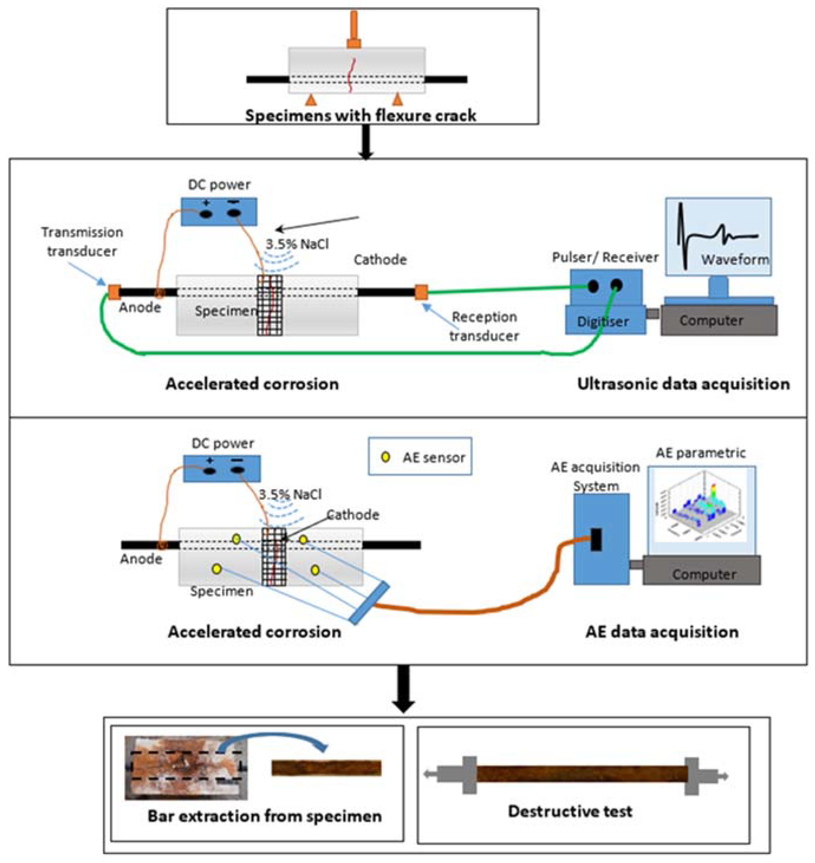
2. Experimental Program
2.1. Specimen Preparation
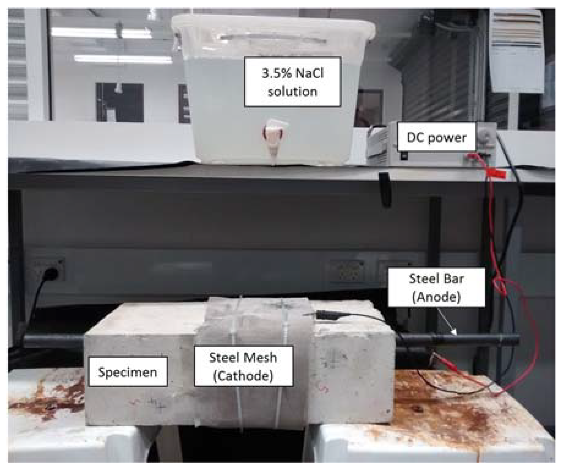
2.2. Accelerated Corrosion
2.3. Guided Wave Ultrasonic Monitoring
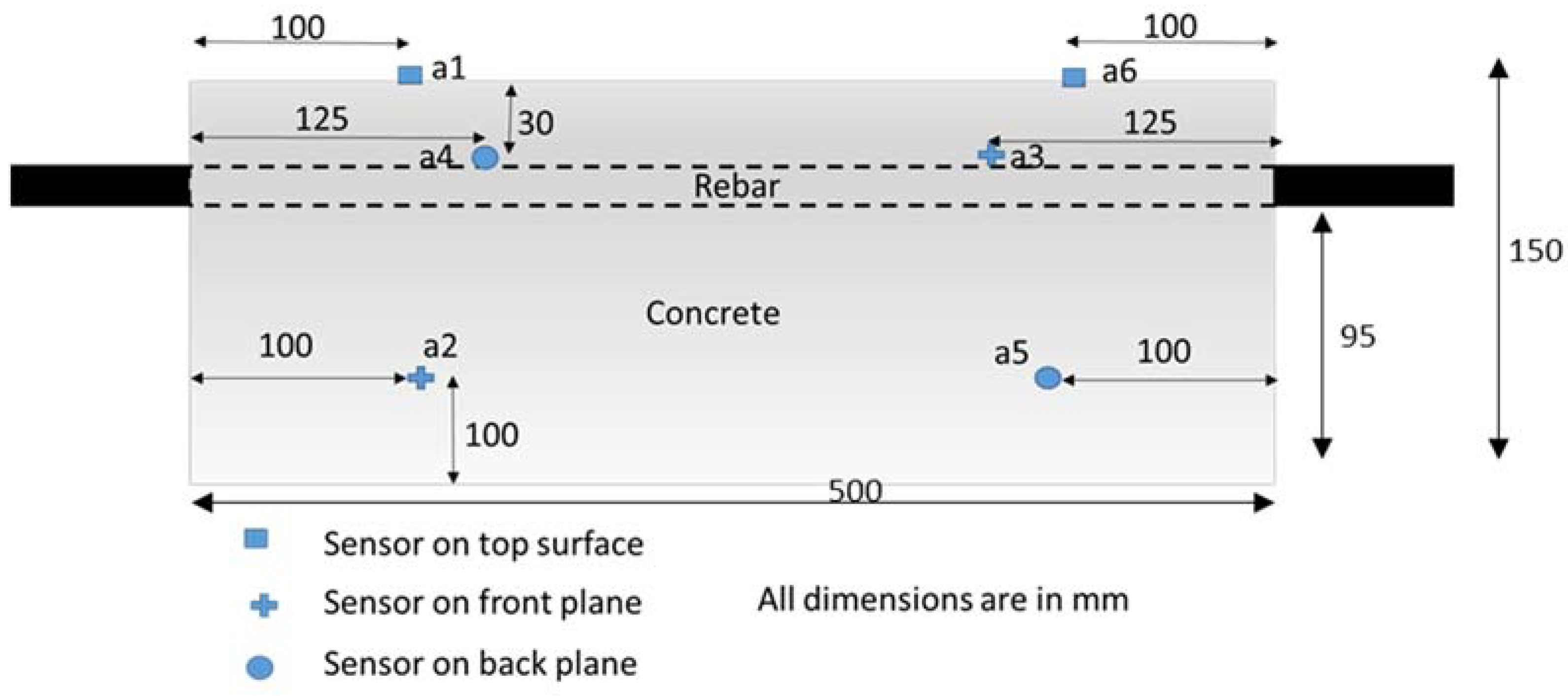
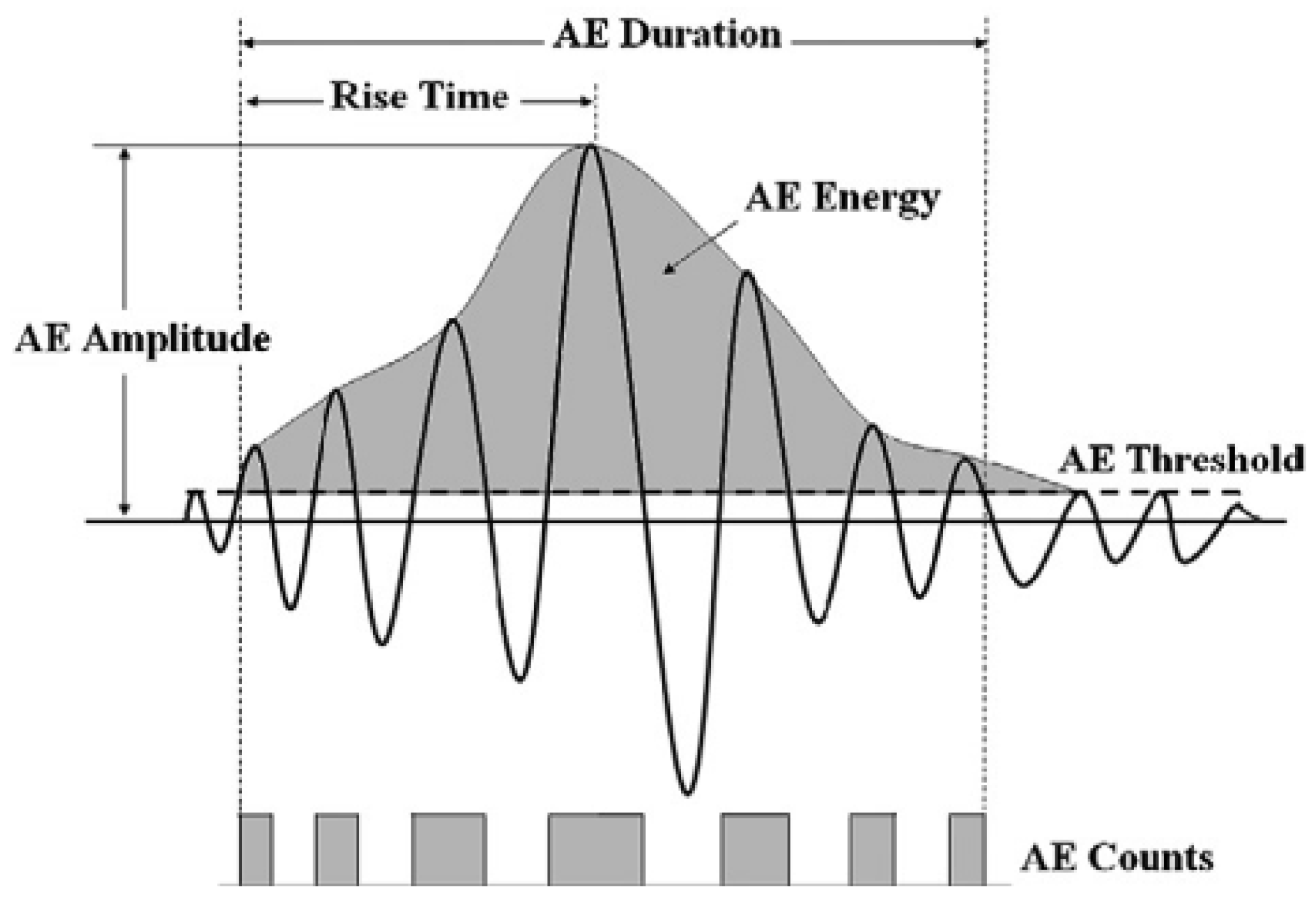
2.4. AE Emission Test
2.5. Destructive Tests
3. Experimental Results
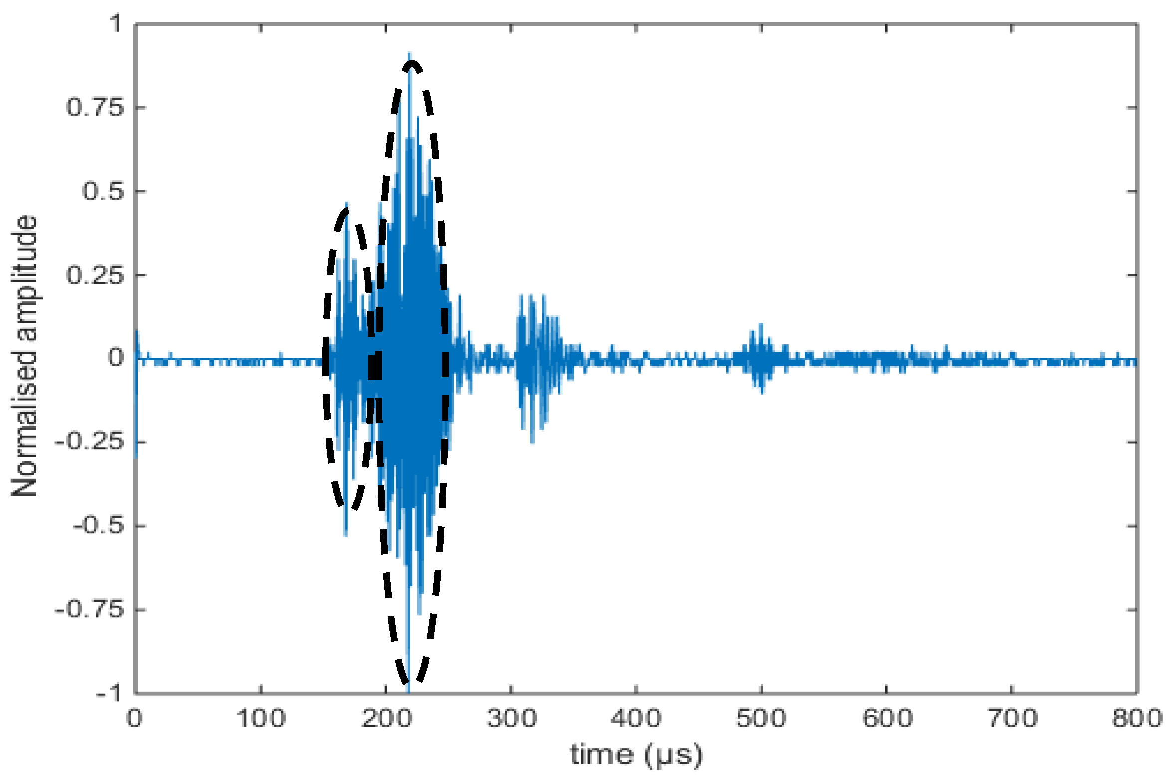
3.1. Time Signal (A-Scan)
3.2. Signal Analysis
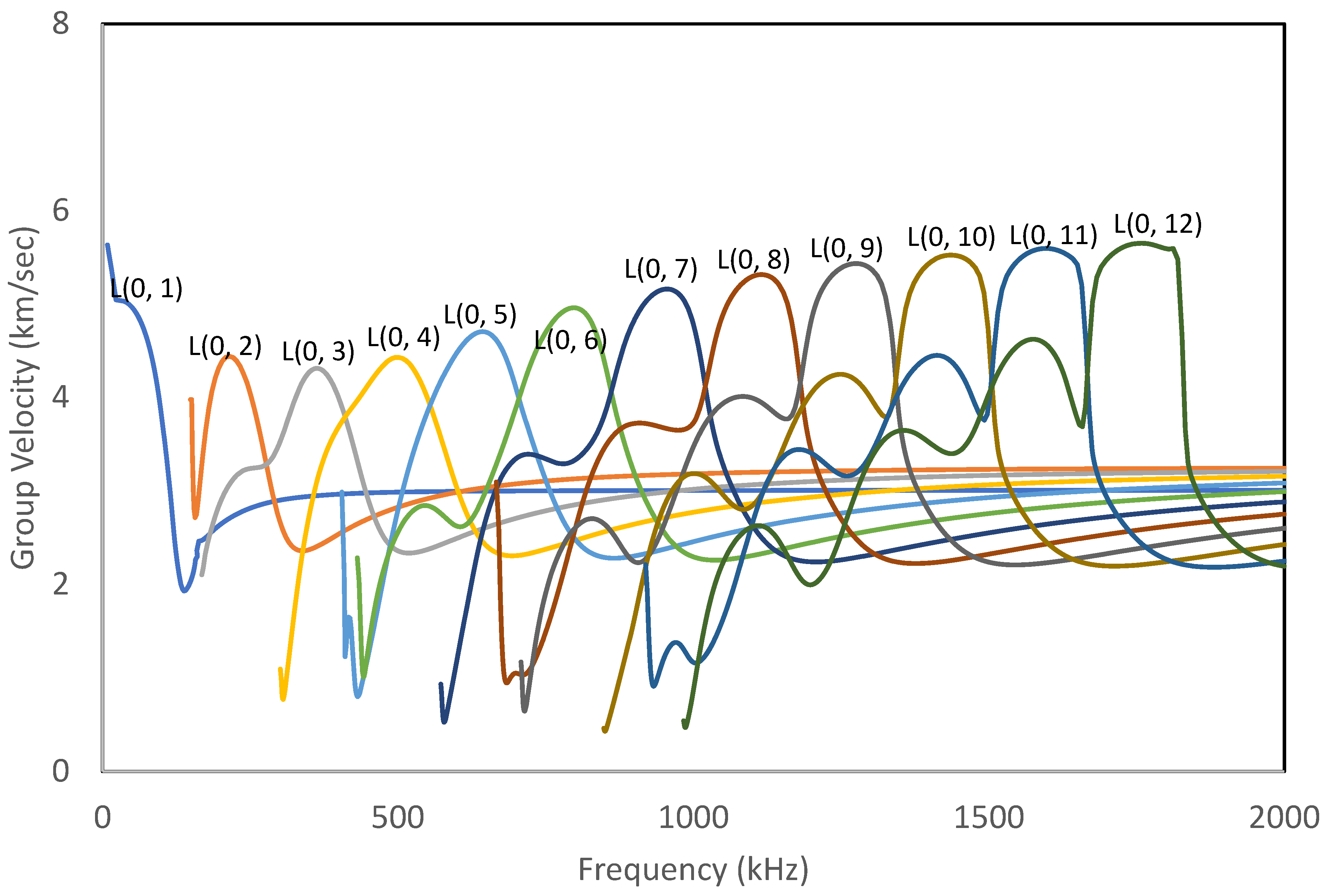
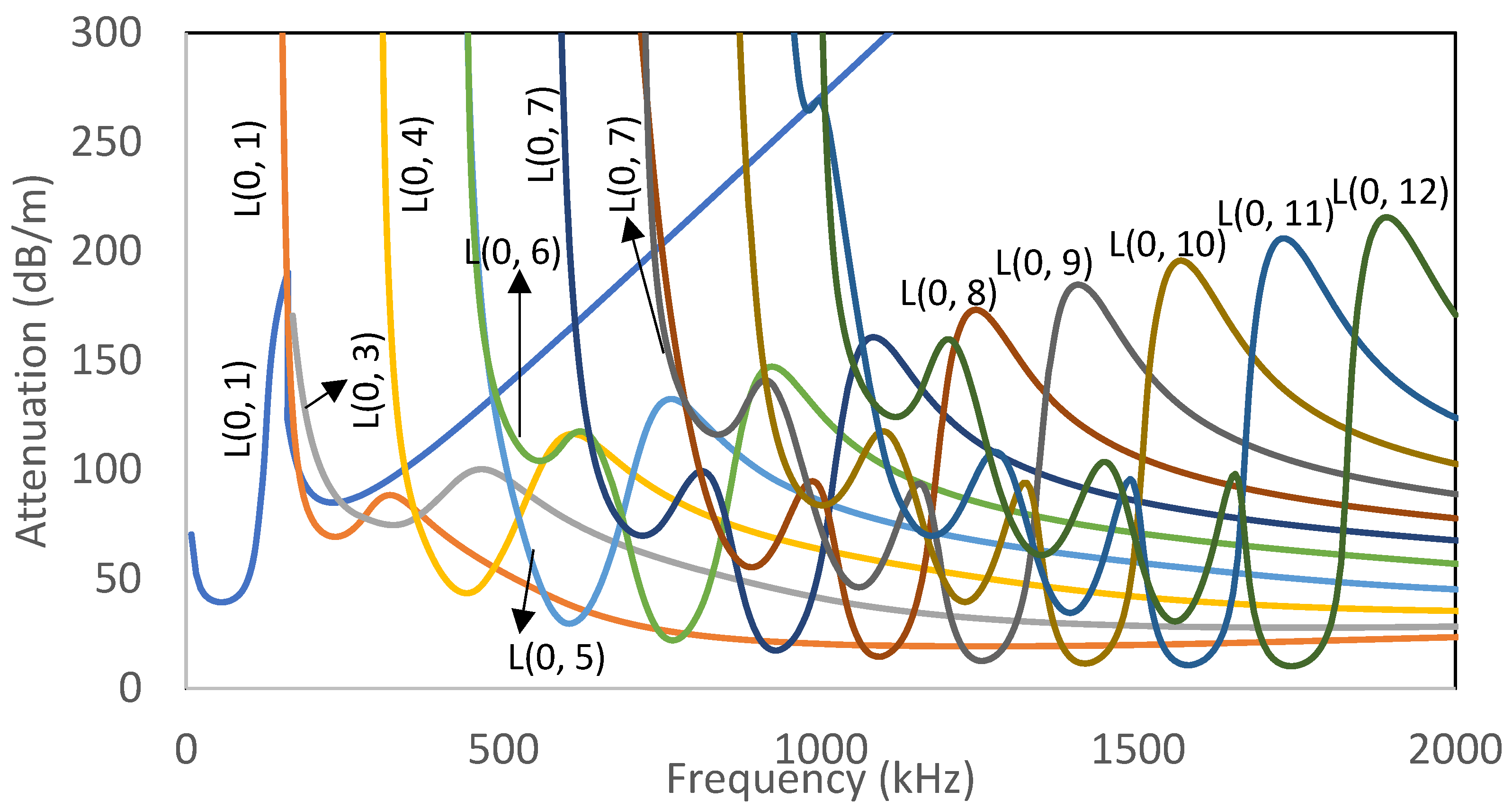
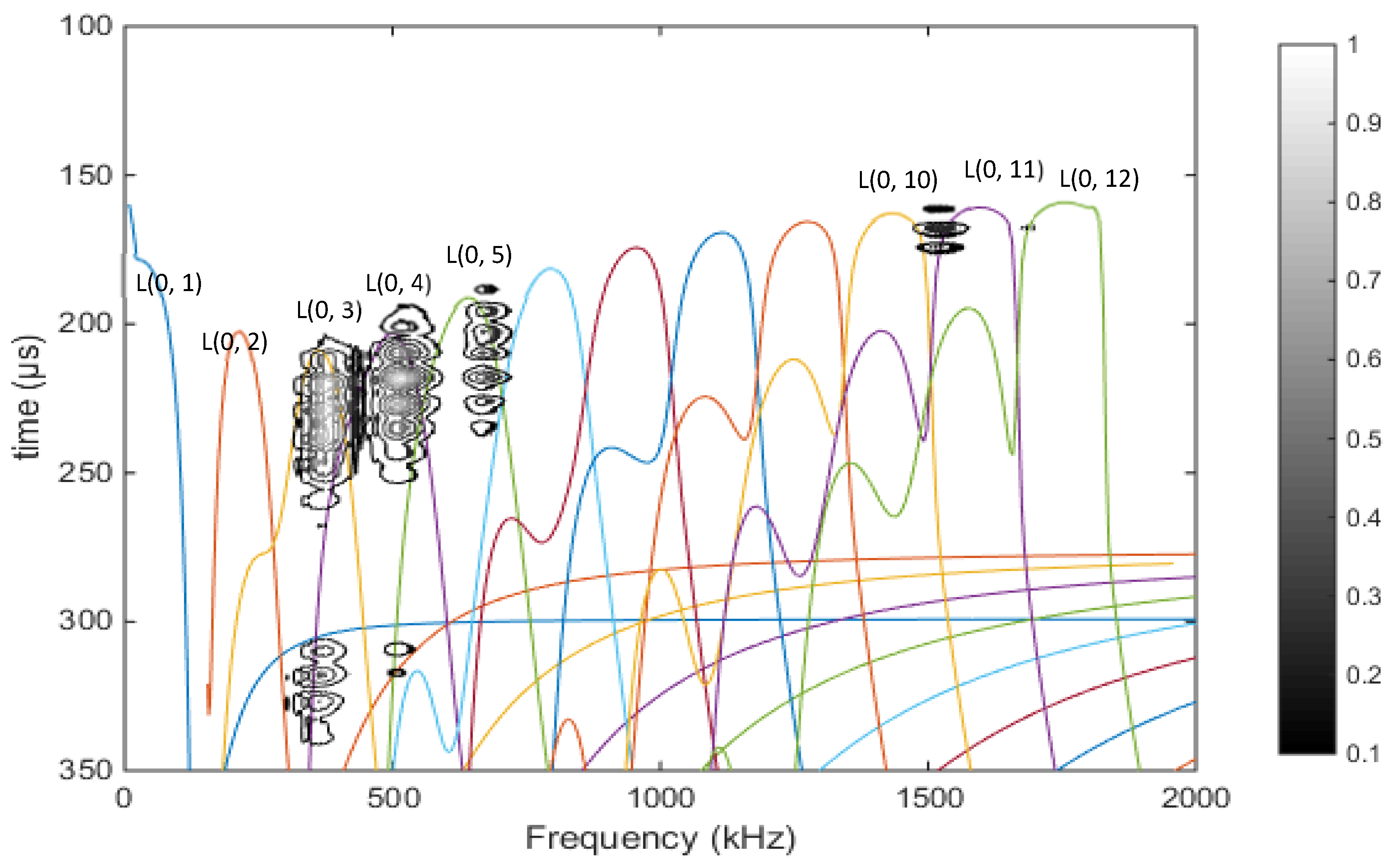
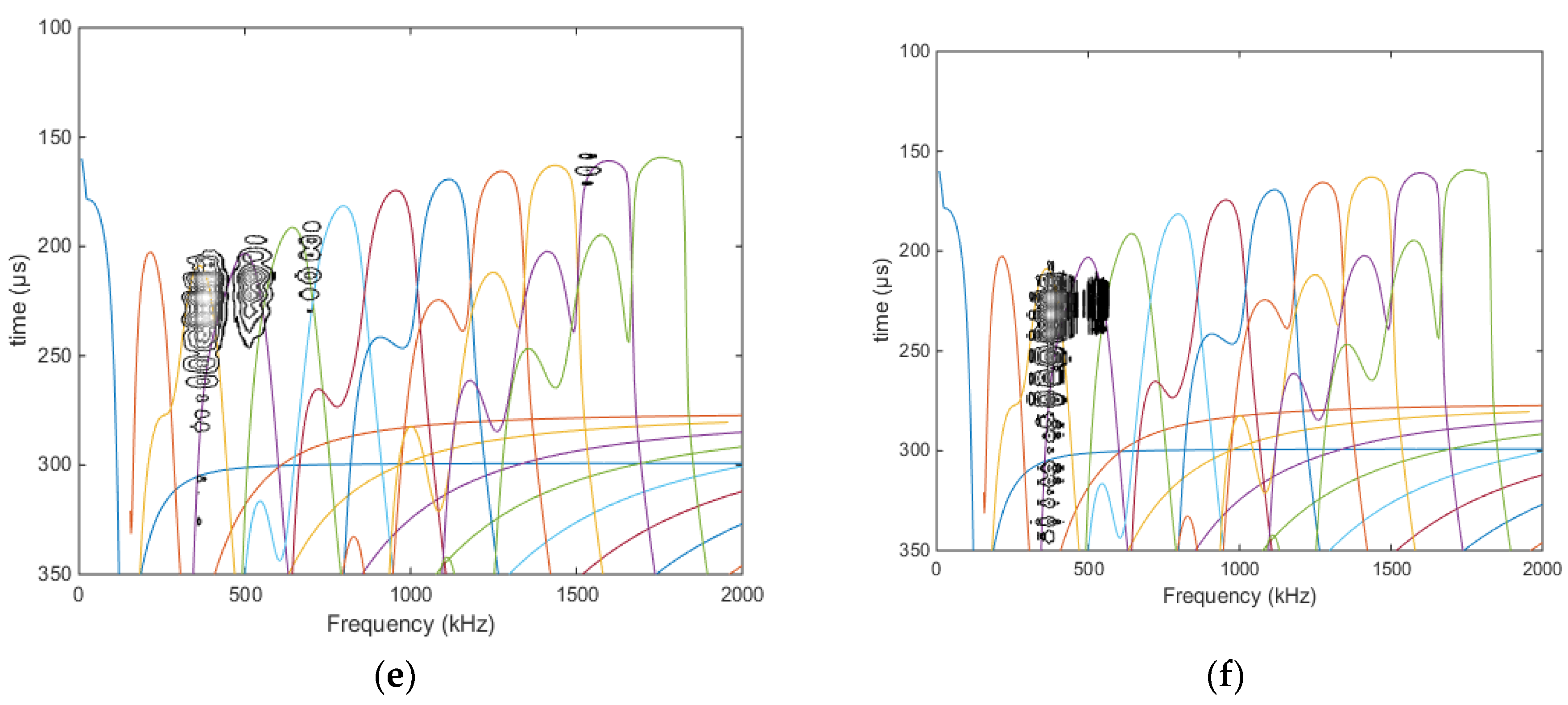
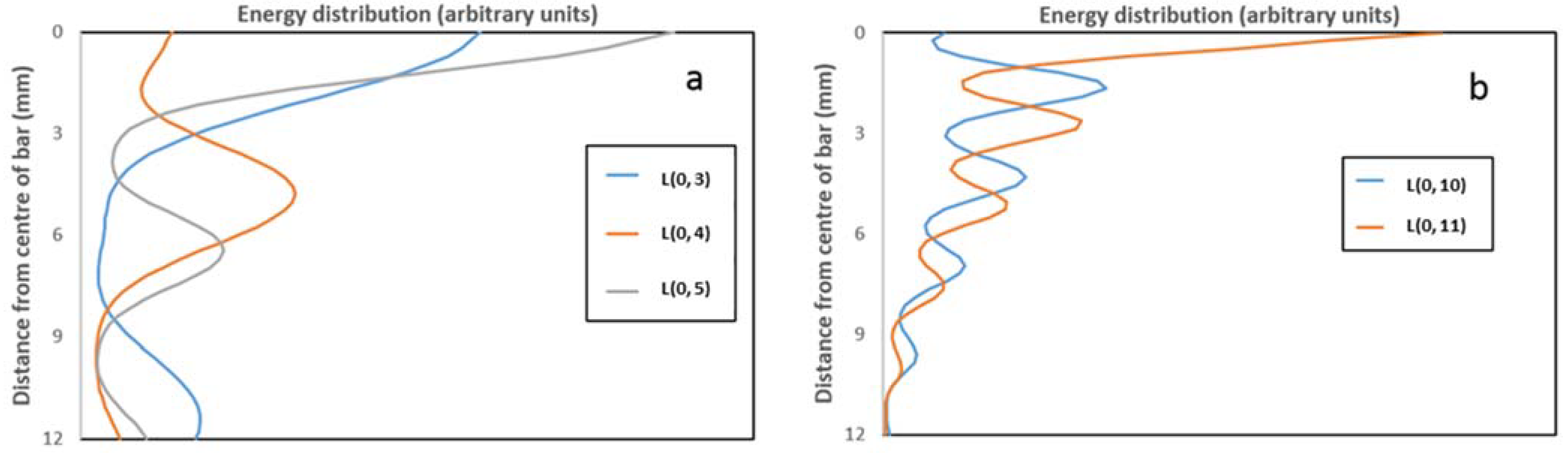
3.3. Guided Wave Modes
3.4. Variation of Guided-Wave Signal with Corrosion
3.5. Acoustic Emission Monitoring
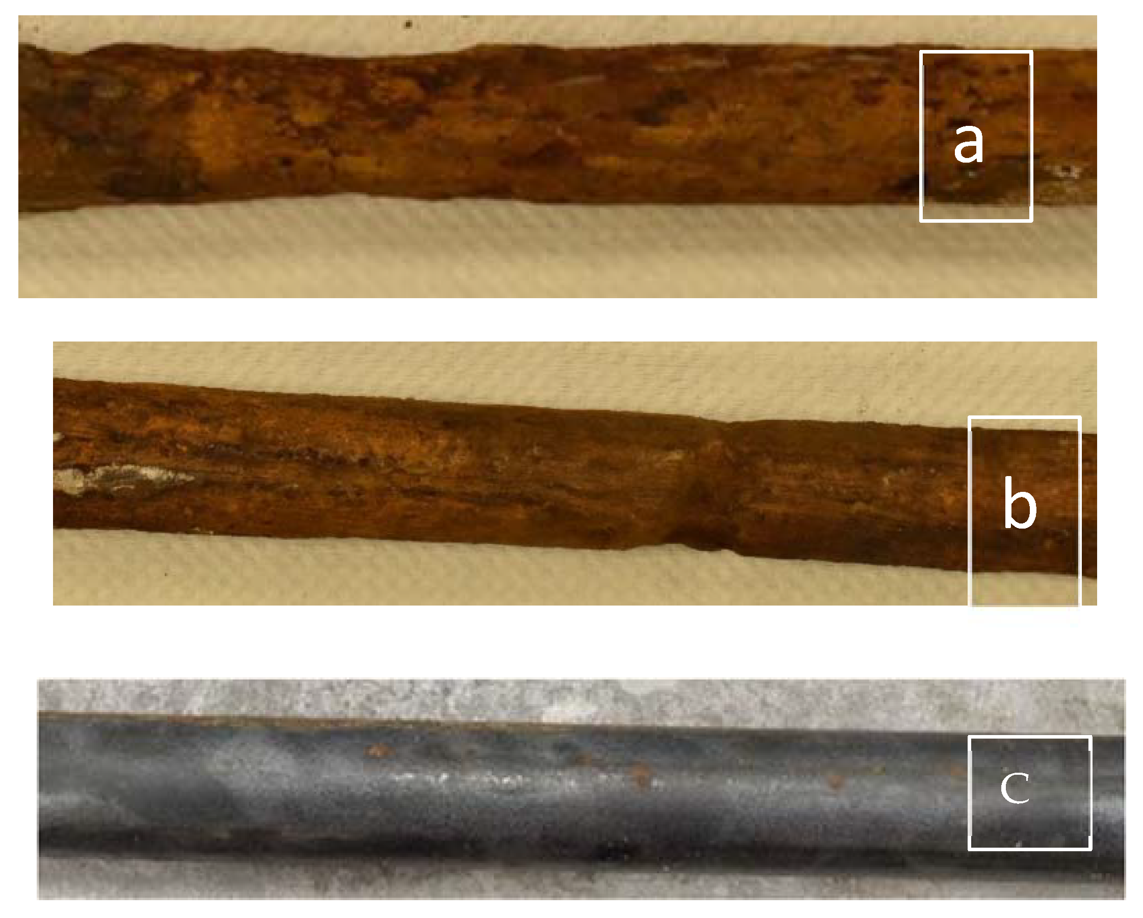
3.6. Destructive Tests
4. Corrosion Classification
5. Conclusions
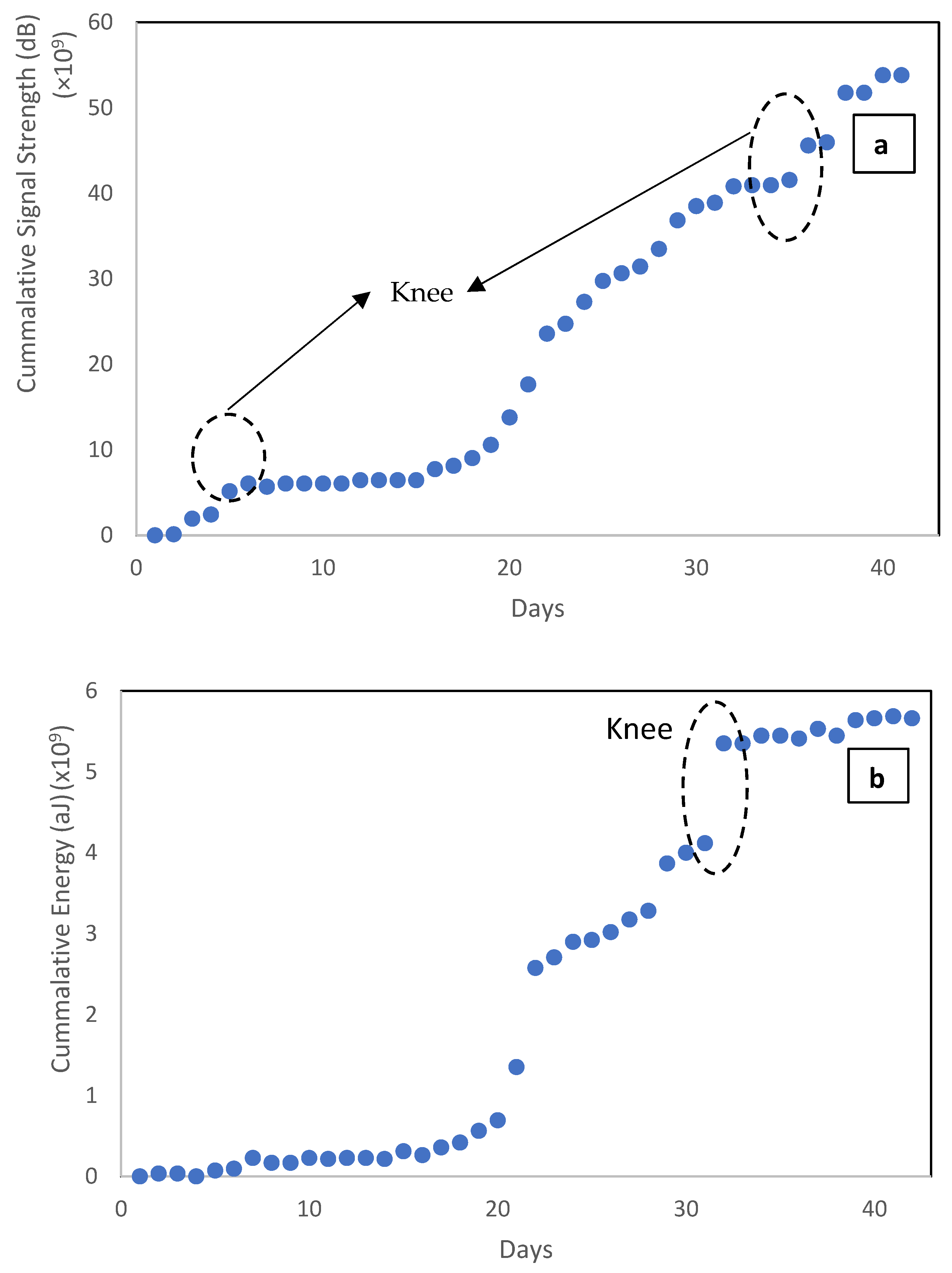
- An initial increase in χRS_norm until day 6 signifies the improvement in signal strength past the onset of corrosion. This can be attributed to the formation of soft corrosion products around the rebar. In this duration, the cumulative AE parametric such as hits, signal strength, and energy were relatively low until this point. This represents the initiation of corrosion.
- After an initial increase in χRS_norm, its magnitude decreased past day 5. This decreasing trend continued until day 15. A steady rise in acoustic parameters in this duration indicates the nucleation of micro-cracks in the concrete surrounding the steel bar. χRS_norm decreased at a steeper gradient until day 34, which indicates the coalescence of micro-cracks to macro-cracks. At this stage, the acoustic parameters increase, indicating the evolution of macro-cracks. Thus, the intermediate stage of corrosion represents the transition of corrosion induction cracking in the concrete from micro-cracks to macro-cracks.
- Beyond day 34, as a consequence of profound pitting on the rebar and cracking in the concrete, the magnitude of χRS_norm was reduced to an insignificant value. During the same period, the increase in acoustic parameters was marginal. This trend continued until the conclusion of the experiment.
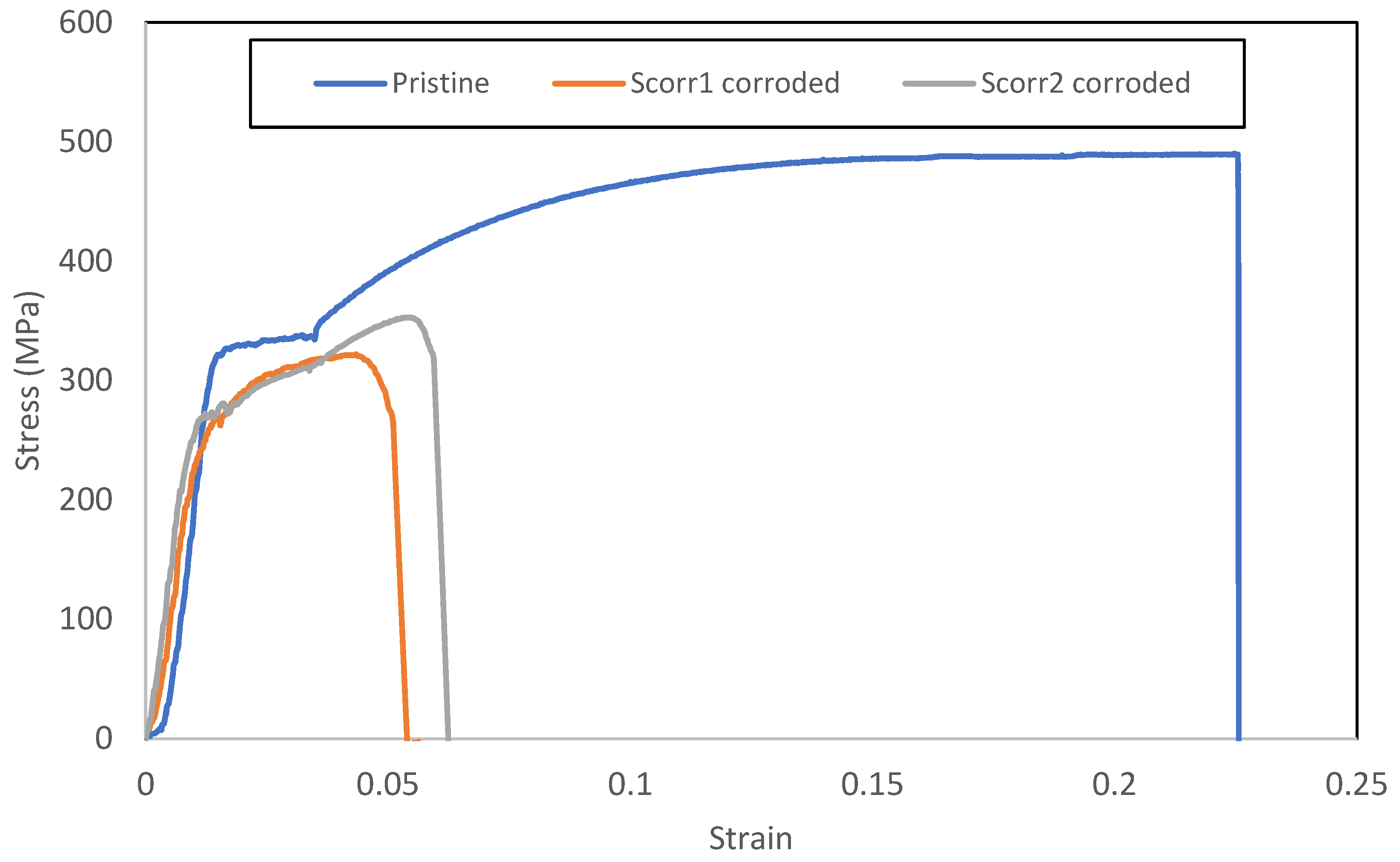
- A reduction in strength and ductility due to corrosion in the specimen was observed. The yield and ultimate strength of the specimen were reduced by 17.8% and 35.28%, respectively, and 15.26% and 21.48%, respectively, for Scorr1 and Scorr2 compared to the pristine specimen. Failure strain was reduced by 75.11% and 72.28%, respectively, for Scorr1 and Scorr2 due to corrosion.
Author Contributions
Funding
Institutional Review Board Statement
Informed Consent Statement
Conflicts of Interest
References
- Mistri, A.; Bhattacharyya, S.K.; Dhami, N.; Mukherjee, A.; Barai, S.V. A Review on Different Treatment Methods for Enhancing the Properties of Recycled Aggregates for Sustainable Construction Materials. Constr. Build. Mater. 2020, 233, 117894. [Google Scholar] [CrossRef]
- Australian Local Government Association. 2015 National State of the Assets Report. Available online: https://alga.com.au/national-state-of-the-assets-report-2015/ (accessed on 7 May 2022).
- Wong, H.S.; Angst, U.M.; Geiker, M.R.; Isgor, O.B.; Elsener, B.; Michel, A.; Alonso, M.C.; Correia, M.J.; Pacheco, J.; Gulikers, J. Methods for Characterising the Steel–Concrete Interface to Enhance Understanding of Reinforcement Corrosion: A Critical Review by Rilem Tc 262-Sci. Mater. Struct. 2022, 55, 124. [Google Scholar] [CrossRef]
- Ahmad, S. Reinforcement Corrosion in Concrete Structures, Its Monitoring and Service Life Prediction––a Review. Cem. Concr. Compos. 2003, 25, 459–471. [Google Scholar] [CrossRef]
- Liu, Y. Modeling the Time-to Corrosion Cracking of the Cover Concrete in Chloride Contaminated Reinforced Concrete Structures. Ph.D. Thesis, Virginia Tech, Blacksburg, VA, USA, October 1996. [Google Scholar]
- Andrade, C.; Alonso, C.; Molina, F.J. Cover Cracking as a Function of Bar Corrosion: Part I-Experimental Test. Mater. Struct. 1993, 26, 453–464. [Google Scholar] [CrossRef]
- Gadve, S.; Mukherjee, A.; Malhotra, S.N. Corrosion of Steel Reinforcements Embedded in Frp Wrapped Concrete. Constr. Build. Mater. 2009, 23, 153–161. [Google Scholar] [CrossRef]
- Simon, P.D. Improved Current Distribution Due to a Unique Anode Mesh Placement in a Steel Reinforced Concrete Parking Garage Slab Cp System. In Proceedings of the CORROSION 2004, New Orleans, LA, USA, 28 March–2 April 2004. [Google Scholar]
- Broomfield, J.P. Corrosion of Steel in Concrete: Understanding, Investigation and Repair; CRC Press: Oxon, UK, 2003. [Google Scholar]
- Liang, M.-T.; Su, P.-J. Detection of the Corrosion Damage of Rebar in Concrete Using Impact-Echo Method. Cem. Concr. Res. 2001, 31, 1427–1436. [Google Scholar] [CrossRef]
- Bagavathiappan, S.; Lahiri, B.B.; Saravanan, T.; Philip, J.; Jayakumar, T. Infrared Thermography for Condition Monitoring—A Review. Infrared Phys. Technol. 2013, 60, 35–55. [Google Scholar] [CrossRef]
- Elsener, B.; Andrade, C.; Gulikers, J.; Polder, R.; Raupach, M. Hall-Cell Potential Measurements—Potential Mapping on Reinforced Concrete Structures. Mater. Struct. 2003, 36, 461–471. [Google Scholar] [CrossRef]
- Song, H.-W.; Saraswathy, V. Corrosion Monitoring of Reinforced Concrete Structures-A. Int. J. Electrochem. Sci. 2007, 2, 1–28. [Google Scholar]
- Achenbach, J. Wave Propagation in Elastic Solids; Elsevier: Amsterdam, The Netherlands, 2012; Volume 16. [Google Scholar]
- Rose, J.L. Ultrasonic Guided Waves in Solid Media; Cambridge University Press: Cambridge, UK, 2014. [Google Scholar]
- Graff, K.F. Wave Motion in Elastic Solids; Courier Corporation: North Chelmsford, MA, USA; Clarendon Press: Oxford, UK, 2012. [Google Scholar]
- Sharma, S.; Mukherjee, A. Monitoring Corrosion in Oxide and Chloride Environments Using Ultrasonic Guided Waves. J. Mater. Civ. Eng. 2011, 23, 207–211. [Google Scholar] [CrossRef]
- Sharma, S.; Mukherjee, A. Longitudinal Guided Waves for Monitoring Chloride Corrosion in Reinforcing Bars in Concrete. Struct. Health Monit. 2010, 9, 555–567. [Google Scholar] [CrossRef]
- Liu, Y.; Ding, W.; Zhao, P.; Qin, L.; Shiotani, T. Research on in-Situ Corrosion Process Monitoring and Evaluation of Reinforced Concrete Via Ultrasonic Guided Waves. Constr. Build. Mater. 2022, 321, 126317. [Google Scholar] [CrossRef]
- Mitra, M.; Gopalakrishnan, S. Guided Wave Based Structural Health Monitoring: A Review. Smart Mater. Struct. 2016, 25, 053001. [Google Scholar] [CrossRef]
- Raghavan, A.; Cesnik, C.E.S. Finite-Dimensional Piezoelectric Transducer Modeling for Guided Wave Based Structural Health Monitoring. Smart Mater. Struct. 2005, 14, 1448. [Google Scholar] [CrossRef]
- Sharma, S.; Mukherjee, A. Ultrasonic Guided Waves for Monitoring the Setting Process of Concretes with Varying Workabilities. Constr. Build. Mater. 2014, 72, 358–366. [Google Scholar] [CrossRef]
- Na, W.B.; Kundu, T.; Ehsani, M.R. Ultrasonic Guided Waves for Steel Bar Concrete Interface Testing. Ariel 2002, 129, 31–248. [Google Scholar]
- Sharma, A.; Sharma, S.; Sharma, S.; Mukherjee, A. Ultrasonic Guided Waves for Monitoring Corrosion of Frp Wrapped Concrete Structures. Constr. Build. Mater. 2015, 96, 690–702. [Google Scholar] [CrossRef]
- Sharma, S.; Mukherjee, A. Monitoring Freshly Poured Concrete Using Ultrasonic Waves Guided through Reinforcing Bars. Cem. Concr. Compos. 2015, 55, 337–347. [Google Scholar] [CrossRef]
- Wu, F.; Chan, H.-L.; Chang, F.-K. Ultrasonic Guided Wave Active Sensing for Monitoring of Split Failures in Reinforced Concrete. Struct. Health Monit. 2015, 14, 439–448. [Google Scholar] [CrossRef]
- Ervin, B.L.; Kuchma, D.A.; Bernhard, J.T.; Reis, H. Monitoring Corrosion of Rebar Embedded in Mortar Using High-Frequency Guided Ultrasonic Waves. J. Eng. Mech. 2009, 135, 9–19. [Google Scholar] [CrossRef]
- Ervin, B.L.; Reis, H. Longitudinal Guided Waves for Monitoring Corrosion in Reinforced Mortar. Meas. Sci. Technol. 2008, 19, 055702. [Google Scholar] [CrossRef]
- Demma, A.; Cawley, P.; Lowe, M.; Roosenbrand, A.G.; Pavlakovic, B. The Reflection of Guided Waves from Notches in Pipes: A Guide for Interpreting Corrosion Measurements. Ndt E Int. 2004, 37, 167–180. [Google Scholar] [CrossRef]
- Pavlakovic, B.N.; Lowe, M.J.S.; Cawley, P. High-Frequency Low-Loss Ultrasonic Modes in Imbedded Bars. J. Appl. Mech. 2001, 68, 67–75. [Google Scholar] [CrossRef]
- Lowe, M.J.S.; Alleyne, D.N.; Cawley, P. Defect Detection in Pipes Using Guided Waves. Ultrasonics 1998, 36, 147–154. [Google Scholar] [CrossRef]
- Sharma, S.; Mukherjee, A. Ultrasonic Guided Waves for Monitoring Corrosion in Submerged Plates. Struct. Control. Health Monit. 2015, 22, 19–35. [Google Scholar] [CrossRef]
- Carbol, L.; Kusák, I.; Martinek, J.; Vojkůvková, P. Influence of Transducer Coupling in Ultrasonic Testing. Paper presented at the NDT in Progress 2015 VIIIth International Workshop. The e-Journal of Nondestructive Testing. Praha; Brno University of Technology, Brno, Czech Republic, 12–14 October 2015. [Google Scholar]
- Cai, D.; Zou, C.; Sun, Z.; Zhou, Q.; Fu, Y.; Li, G. The Influence of Coupling Layer Thickness on Hollow Axles Ultrasonic Testing. In Proceedings of the 2015 International Conference on Control, Automation and Robotics, Singapore, 20–22 May 2015. [Google Scholar]
- Gröchenig, K. Foundations of Time-Frequency Analysis; Springer Science & Business Media: New York, NY, USA, 2013. [Google Scholar]
- Portnoff, M. Time-Frequency Representation of Digital Signals and Systems Based on Short-Time Fourier Analysis. IEEE Trans. Acoust. Speech Signal Process. 1980, 28, 55–69. [Google Scholar] [CrossRef]
- Daubechies, I. The Wavelet Transform, Time-Frequency Localization and Signal Analysis. IEEE Trans. Inf. Theory 1990, 36, 961–1005. [Google Scholar] [CrossRef] [Green Version]
- Prosser, W.H.; Seale, M.D.; Smith, B.T. Time-Frequency Analysis of the Dispersion of Lamb Modes. J. Acoust. Soc. Am. 1999, 105, 2669–2676. [Google Scholar] [CrossRef] [Green Version]
- Abbate, A.; Koay, J.; Frankel, J.; Schroeder, S.C.; Das, P. Signal Detection and Noise Suppression Using a Wavelet Transform Signal Processor: Application to Ultrasonic Flaw Detection. IEEE Trans. Ultrason. Ferroelectr. Freq. Control 1997, 44, 14–26. [Google Scholar] [CrossRef]
- Shelke, A.; Kundu, T.; Amjad, U.; Hahn, K.; Grill, W. Mode-Selective Excitation and Detection of Ultrasonic Guided Waves for Delamination Detection in Laminated Aluminum Plates. IEEE Trans. Ultrason. Ferroelectr. Freq. Control 2011, 58, 567–577. [Google Scholar] [CrossRef]
- Burrows, S.E.; Dixon, S. Defect Detection Using a Scanning Laser Source. In AIP Conference Proceedings 2011; American Institute of Physics: New York, NY, USA, 2011. [Google Scholar]
- Mostavi, A.; Kamali, N.; Tehrani, N.; Chi, S.-W.; Ozevin, D.; Ernesto, J.I. Wavelet Based Harmonics Decomposition of Ultrasonic Signal in Assessment of Plastic Strain in Aluminum. Measurement 2017, 106, 66–78. [Google Scholar] [CrossRef] [Green Version]
- Majhi, S.; Mukherjee, A.; George, N.V.; Uy, B. Corrosion Detection in Steel Bar: A Time-Frequency Approach. Ndt E Int. 2019, 107, 102150. [Google Scholar] [CrossRef]
- Majhi, S.; Mukherjee, A.; George, N.V.; Karaganov, V.; Uy, B. Corrosion monitoring in steel bars using laser ultrasonic guided waves and advanced signal processing. Mech. Syst. Signal Process. 2021, 149, 107176. [Google Scholar] [CrossRef]
- Sharma, A.; Sharma, S.; Sharma, S.; Mukherjee, A. Investigation of Deterioration in Corroding Reinforced Concrete Beams Using Active and Passive Techniques. Constr. Build. Mater. 2018, 161, 555–569. [Google Scholar] [CrossRef]
- Ohtsu, M. Acoustic Emission and Related Non-Destructive Evaluation Techniques in the Fracture Mechanics of Concrete: Fundamentals and Applications; Woodhead Publishing: Duxford, UK, 2015. [Google Scholar]
- Shah, S.G.; Kishen, J.C. Use of acoustic emissions in flexural fatigue crack growth studies on concrete. Eng. Fract. Mech. 2012, 87, 36–47. [Google Scholar] [CrossRef]
- Grosse, C.U.; Ohtsu, M. Acoustic Emission Testing; Springer Science & Business Media: Berlin/Heidelberg, Germany, 2008. [Google Scholar]
- Di Benedetti, M.; Loreto, G.; Matta, F.; Nanni, A. Acoustic Emission Monitoring of Reinforced Concrete under Accelerated Corrosion. J. Mater. Civ. Eng. 2013, 25, 1022–1029. [Google Scholar] [CrossRef]
- Di Benedetti, M.; Loreto, G.; Matta, F.; Nanni, A. Acoustic Emission Historic Index and Frequency Spectrum of Reinforced Concrete under Accelerated Corrosion. J. Mater. Civ. Eng. 2014, 26, 04014059. [Google Scholar] [CrossRef]
- Zaki, A.; Chai, H.K.; Behnia, A.; Aggelis, D.G.; Tan, J.Y.; Ibrahim, Z. Monitoring Fracture of Steel Corroded Reinforced Concrete Members under Flexure by Acoustic Emission Technique. Constr. Build. Mater. 2017, 136, 609–618. [Google Scholar] [CrossRef] [Green Version]
- Yuyama, S.; Nishida, T. Acoustic Emission Evaluation of Corrosion Damages in Buried Pipes of Refinery. J. Acoust. Emisison 2003, 21, 187–194. [Google Scholar]
- Ohtsu, M.; Tomoda, Y. Phenomenological Model of Corrosion Process in Reinforced Concrete Identified by Acoustic Emission. ACI Mater. J. 2008, 105, 194–199. [Google Scholar]
- Sharma, A.; Sharma, S.; Sharma, S.; Mukherjee, A. Monitoring Invisible Corrosion in Concrete Using a Combination of Wave Propagation Techniques. Cem. Concr. Compos. 2018, 90, 89–99. [Google Scholar] [CrossRef]
- Uddin, A.K.M.F.; Numata, K.; Shimasaki, J.; Shigeishi, M.; Ohtsu, M. Mechanisms of Crack Propagation Due to Corrosion of Reinforcement in Concrete by Ae-Sigma and Bem. Constr. Build. Mater. 2004, 18, 181–188. [Google Scholar] [CrossRef]
- Sahu, S.S.; Panda, G.; George, N.V. An Improved S-Transform for Time-Frequency Analysis. In Proceedings of the 2009 IEEE International Advance Computing Conference, (IACC) 2009, Patiala, India, 6–7 March 2009. [Google Scholar]
- Agrawal, S.; George, N.V.; Prashant, A. Gpr Data Analysis of Weak Signals Using Modified S-Transform. Geotech. Geol. Eng. 2015, 33, 1167–1182. [Google Scholar] [CrossRef]
- Pavlakovic, B.; Lowe, M.; Alleyne, D.; Cawley, P. Disperse: A General Purpose Program for Creating Dispersion Curves. In Review of Progress in Quantitative Nondestructive Evaluation; Plenum Press: New York, NY, USA, 1997; pp. 185–192. [Google Scholar]
- Beard, M.D.; Lowe, M.J.S.; Cawley, P. Ultrasonic Guided Waves for Inspection of Grouted Tendons and Bolts. J. Mater. Civ. Eng. 2003, 15, 212–218. [Google Scholar] [CrossRef]
- Zaki, A.; Chai, H.K.; Aggelis, D.G.; Alver, N. Non-Destructive Evaluation for Corrosion Monitoring in Concrete: A Review and Capability of Acoustic Emission Technique. Sensors 2015, 15, 19069–19101. [Google Scholar] [CrossRef]
- Kawasaki, Y.; Wakuda, T.; Kobarai, T.; Ohtsu, M. Corrosion Mechanisms in Reinforced Concrete by Acoustic Emission. Constr. Build. Mater. 2013, 48, 1240–1247. [Google Scholar] [CrossRef]
- Sriramadasu, R.C.; Banerjee, S.; Lu, Y. Sensitivity of Longitudinal Guided Wave Modes to Pitting Corrosion of Rebars Embedded in Reinforced Concrete. Constr. Build. Mater. 2020, 239, 117855. [Google Scholar] [CrossRef]
- Rajeshwara, C.S.; Banerjee, S.; Lu, Y. Identification of Zero Effect State in Corroded Rcc Structures Using Guided Waves and Embedded Piezoelectric Wafer Transducers (Pwt). Procedia Eng. 2017, 188, 209–216. [Google Scholar] [CrossRef]


| Constituent | Cement | Fine Aggregates | Coarse Aggregates | Water-Cement Ratio |
|---|---|---|---|---|
| Composition | 1 | 1.6 | 3.4 | 0.5 |
| Mass (kg/m3) | 370 | 591 | 1255 | 185 |
| Threshold | Timing Parameters | ||
|---|---|---|---|
| PDT | HDT | HLT | |
| 40 dB | 200 | 800 | 1000 |
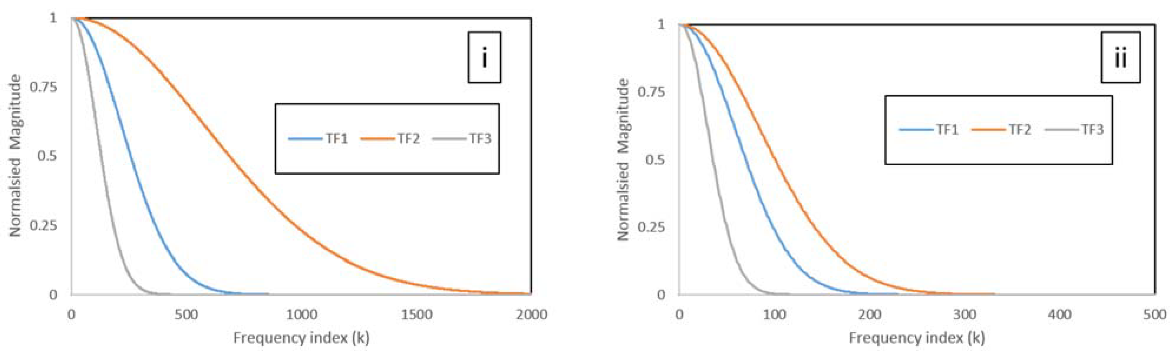
| SL No | a | b | Case |
|---|---|---|---|
| 1 | 10 | 0.5 | TF1 |
| 2 | 1 | 0.1 | TF2 |
| 3 | 20 | 1 | TF3 |
| Properties | Steel | Concrete |
|---|---|---|
| Modulus, E (GPa) | 210 | 29.6 |
| Density (ρ) (kg/m3) | 7932 | 2200 |
| Longitudinal attenuation (np/wl) | 0.003 | 0.2 |
| Shear attenuation (np/wl) | 0.008 | 0.5 |
| Poisson’s ratio | 0.286 | 0.27 |
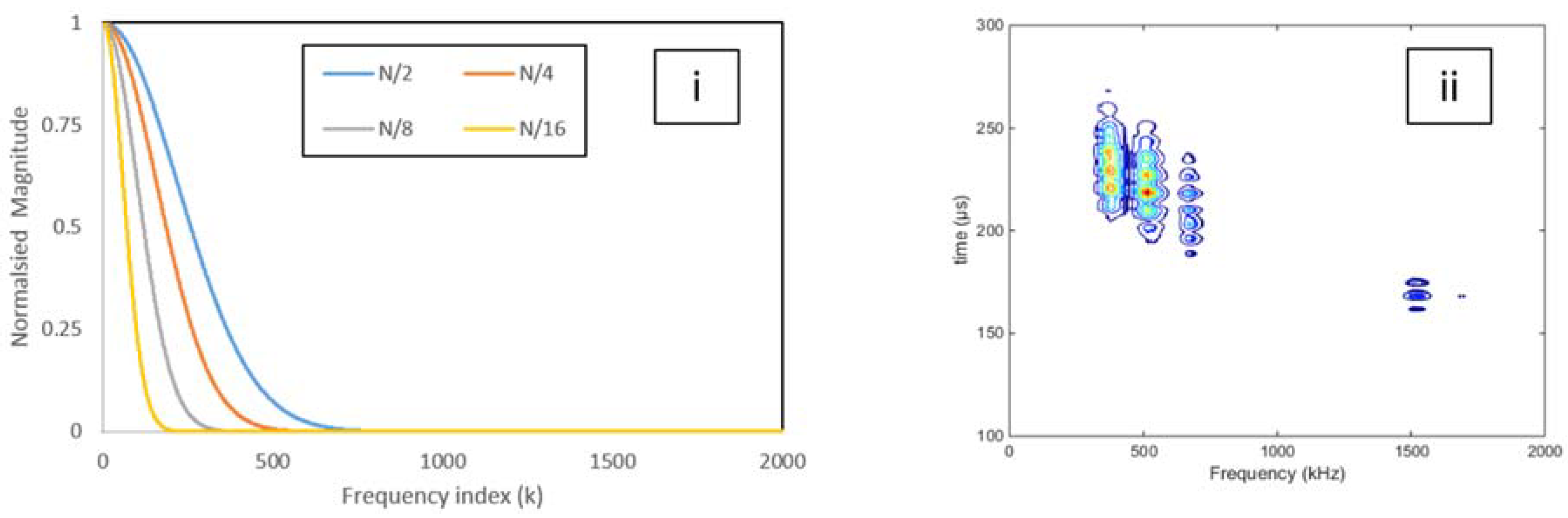
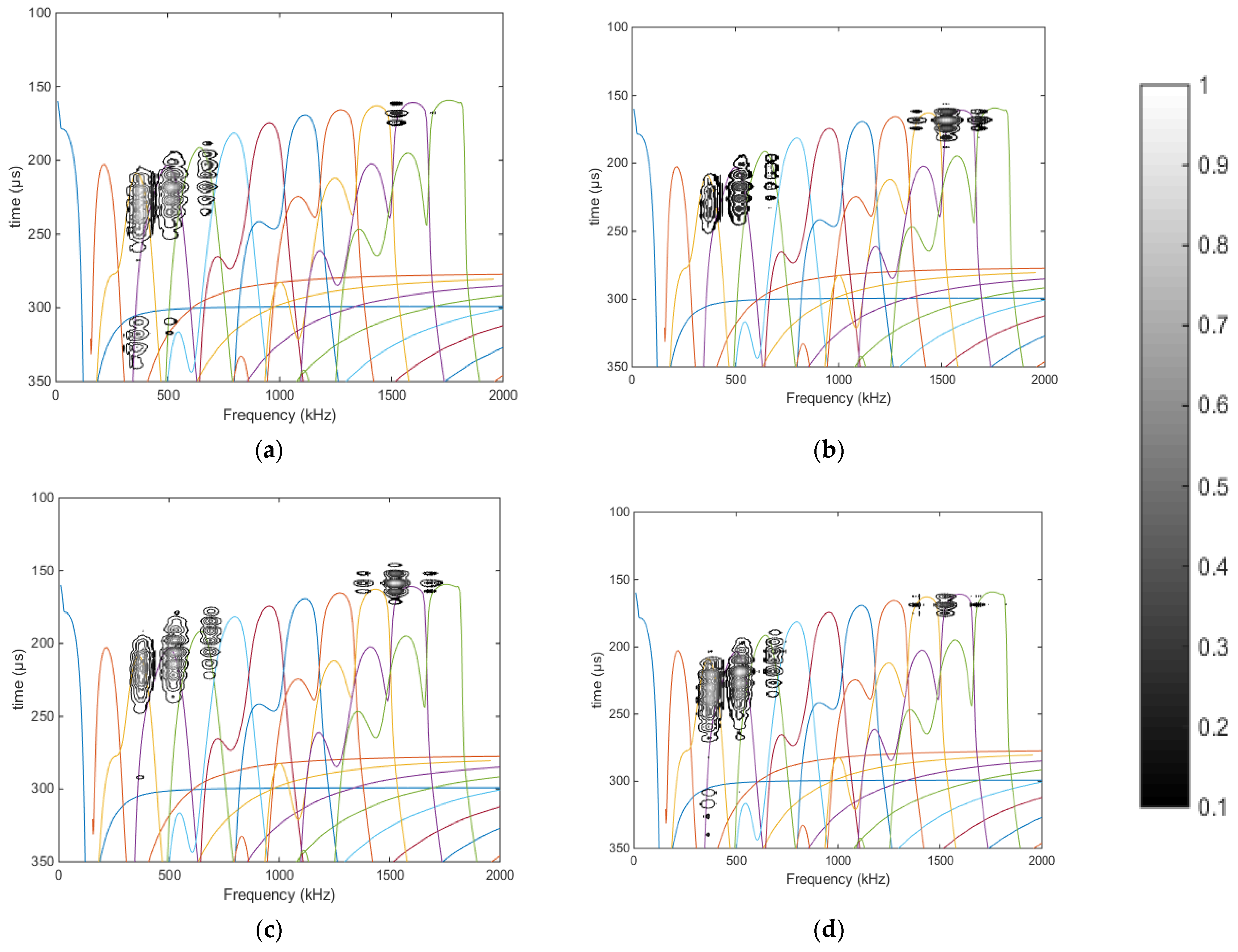
| Zone | tl (μs) | th (μs) | fl (kHz) | fh (kHz) |
|---|---|---|---|---|
| Zone A | 160 | 180 | 220 | 770 |
| Zone B | 190 | 280 | 1220 | 1650 |
Publisher’s Note: MDPI stays neutral with regard to jurisdictional claims in published maps and institutional affiliations. |
© 2022 by the authors. Licensee MDPI, Basel, Switzerland. This article is an open access article distributed under the terms and conditions of the Creative Commons Attribution (CC BY) license (https://creativecommons.org/licenses/by/4.0/).
Share and Cite
Majhi, S.; Asilo, L.K.; Mukherjee, A.; George, N.V.; Uy, B. Multimodal Monitoring of Corrosion in Reinforced Concrete for Effective Lifecycle Management of Built Facilities. Sustainability 2022, 14, 9696. https://doi.org/10.3390/su14159696
Majhi S, Asilo LK, Mukherjee A, George NV, Uy B. Multimodal Monitoring of Corrosion in Reinforced Concrete for Effective Lifecycle Management of Built Facilities. Sustainability. 2022; 14(15):9696. https://doi.org/10.3390/su14159696
Chicago/Turabian StyleMajhi, Subhra, Leonarf Kevin Asilo, Abhijit Mukherjee, Nithin V. George, and Brian Uy. 2022. "Multimodal Monitoring of Corrosion in Reinforced Concrete for Effective Lifecycle Management of Built Facilities" Sustainability 14, no. 15: 9696. https://doi.org/10.3390/su14159696
APA StyleMajhi, S., Asilo, L. K., Mukherjee, A., George, N. V., & Uy, B. (2022). Multimodal Monitoring of Corrosion in Reinforced Concrete for Effective Lifecycle Management of Built Facilities. Sustainability, 14(15), 9696. https://doi.org/10.3390/su14159696