Research on the Prediction Model of the Used Car Price in View of the PSO-GRA-BP Neural Network

Abstract

As the mobile Internet improves by leaps and bounds, the model of traditional offline used car trading has gradually lost the ability to live up to the needs of consumers, and online used car trading platforms have emerged as the times require. Second-hand car price assessment is the premise of second-hand car trading, and a reasonable price can reflect the objective, fair, and true nature of the second-hand car market. In order to standardize the evaluation standards of used car prices and improve the accuracy of used car price forecasts, the linear correlation between vehicle parameters, vehicle conditions, and transaction factors and used car price was comprehensively investigated, grey relational analysis was applied to filter the feature variables of factors affecting used car price, the traditional BP neural network was also optimized by combining the particle swarm optimization algorithm, and a used car price prediction method based on PSO-GRA-BPNN was proposed. The results show that only the correlation coefficient of new car price, engine power, and used car price is greater than 0.6, which has a certain linear correlation. The correlation between new car price, displacement, mileage, gearbox type, fuel consumption, and registration time on used car prices is greater than 0.7, and the impact of other indicators on used car prices is negligible. Compared with the traditional BPNN model and the multiple linear regression, random forest, and support vector machine regression models proposed by other researchers, the MAPE of the PSO-GRA-BPNN model proposed in this paper is 3.936%, which is 30.041% smaller than the error of the other three models. The MAE of the PSO-GRA-BPNN model is 0.475, which is a maximum reduction of 0.622 compared to the other three models. R can reach up to 0.998, and R² can reach 0.984. Although the longest training time is 94.153 s, the overall prediction effect is significantly better than other used car price prediction models, providing a new idea and method for used car evaluation.

1. Introduction

With an increasingly flourishing quantity of private cars and the advancement of the used car market, used cars have to become the top priority for buyers. The price of a used car is an important aspect of a successful transaction for both buyers and sellers. For car buyers, acknowledging the price of used cars allows for trading with peace of mind; for car sellers, evaluating the residual value of used cars can help them set prices reasonably. In other commodity markets, such as stock markets [1], gold markets [2], and agricultural markets [3], price forecasting has been a key focus of research. Used cars, as a commodity, can be priced in the same way. However, used car transactions are much more complex than other commodity transactions, as the sale price is influenced not only by the basic features of the car itself, such as brand, power, and structure, but also by the condition of the car, such as mileage and usage time, as well as a lack of presently available methods determining which factors hit the sale price most dramatically [4]. At the same time, online transactions also make it difficult to assess the price of used cars. Used cars are experience goods. Different from search goods, it is difficult for consumers to make a purchase decision based on the vehicle configuration. The actual user experience has a big impact on the purchase. This exacerbates the difficulty of predicting used car prices accurately. Therefore, how to screen the characteristic variables that affect the price of used cars and improve the accuracy of price prediction of used cars is of great significance for fair transactions between buyers and sellers and the sustainable and healthy development of the used car market [5,6,7,8,9,10].

Traditionally, used car price appraisal methods include the replacement cost method, the present value of earnings method, the current market value method, and the liquidation price method. However, the traditional appraisal methods are difficult to select uniform indicators for and overly rely on the subjective judgment of appraisers, which is beyond the limits of online trading in the used car market. On the basis of the replacement cost method, Tan et al. [11] built a method based on the AHP used electric vehicle value system, but the mature used pure electric vehicle market has not yet formed, and it cannot be revised and improved through a large amount of actual transaction data. Chen et al. [12] conducted an empirical investigation and compared the two techniques, linear regression and random forest. This shows that the latter is the best algorithm for dealing with complex models with a large number of variables and data. However, it lacks a clear benefit when dealing with effortless models with fewer variables. The mean NMSE of the sample data fluctuates around 0.3. It can be seen that the existing used car price prediction methods are not ideal, so it is necessary to find a reasonable, efficient, scientific, and accurate method.

Artificial neural networks (ANN), fuzzy logic systems (FLS), and evolutionary algorithms (EA), the most quickly emerging fields in computing intelligence, can be used to solve a variety of prediction and optimization challenges [13,14,15]. The BP neural network (BPNN) is a typical ANN that does not rely on any empirical formula and can automatically generalize rules to existing data to obtain the intricate patterns of the data, which is suitable for building multi-factor non-linear forecasting models such as those for used cars. Wu et al. [16] compared a BPNN for used car price prediction with the proposed ANFIS. The results showed that when three feature variables are input, the prediction accuracy of the BPNN is prior to the latter counterpart. Zhou [17] introduced the BPNN to establish a valuation model, reducing the subjectivity and randomness amid the valuation process. It showed that the price evaluation predicted by the BPNN is closer to the actuality, with a maximum error of 3.04%, indicating the reliability and applicability of the model.

When the BPNN algorithm is unable to find the global optimal solution to a complex non-linear function, it falls back on local search, which can easily lead to training failure due to local optima. Furthermore, the predictability of the BPNN is influenced by its trainability. During each training session, the BPNN’s initial weights and thresholds are created at random, resulting in predictions that are not accurate in terms of actual values. Zhang et al. [18] gave a general mathematical expression for the constrained optimization of the BPNN, and by adjusting the input values of the BPNN, the output values can be made optimal, thus avoiding falling into a local optimum solution. Sun et al. [19] used the randomness of the Monte Carlo method to select the optimal number of hidden neurons in the BPNN. This method effectively reduces the number of operations for calculating the number of hidden layers, and the relative error of the model is maintained at about 0.6%. To create a hybrid GA-BP model, Han et al. [20] used a genetic algorithm to optimize the weights and thresholds of the BPNN. The relative errors of the two sets of verified data were found to be 3.4, 1.9, and 3.1%, respectively. The theoretical precision is pretty great. The genetic algorithm is a popular evolutionary optimization approach, but the series of processes involved in network optimization is more complicated, which significantly increases the network’s training time and makes the model more complex. Particle swarm optimization (PSO) can be employed in addition to the genetic algorithm to optimize the network. Without the need to operate on the function gradient, PSO can substitute normal gradient descent and improve the model’s global optimization performance, reducing the network’s training time and increasing the algorithm’s efficiency [21]. Ren et al. [22] used the PSO method to improve the BPNN model’s weights and thresholds, as well as continuously adjust model parameters and functions. The results showed that the PSO-BPNN model performs better than the normal BPNN model, thereby overcoming the BPNN’s flaws. By integrating the BPNN with a strong particle swarm optimization technique, Mohamad et al. [23] avoided becoming stuck in local minima. The R values of the PSO-BPNN model’s training and testing datasets are 0.988 and 0.999, respectively, showing that the model’s performance prediction performs well. As a result, to increase the BPNN’s forecast accuracy for used vehicle pricing, this research looks at how the PSO approach may be utilized to improve the BPNN.

The choice of input feature variables, as well as the optimization of model parameters, is an important element in influencing the BPNN model’s prediction accuracy. When all of the variables that influence the price of used automobiles are employed as feature variables in the prediction model, not only does the modeling efficiency suffer, but the model’s forecast accuracy suffers as well. As a result, the model’s feature variables must be checked ahead of time. The expert scoring approach, hierarchical analysis method, and principal component analysis method are some of the other ways of determining the weights of the characteristic variables. These methods typically require the artificial derivation of indicator weight coefficients or rely on a huge amount of sample data, resulting in less objective outcomes [24,25,26]. However, grey relation analysis (GRA) is used to make up for the shortcomings of these methods. Yao et al. [27] introduced grey relation analysis to describe the internal relationship between features from geometric similarity and discussed the classification ability of feature combination and single feature. An improved feature selection method based on a single rule algorithm is proposed. The results showed that this method is superior to other similar feature selection methods in classification performance. Javanmardi et al. [28] argued that the GRA-based method does not require a comprehensive database of classification rules, can effectively deal with the uncertainty of complex systems, and can flexibly evaluate the ambiguity of multi-factor causality. Wei [29] used GRA to create an optimization model that can effectively solve multi-attribute decision problems using intuitive fuzzy information by determining the weights of each attribute. The extent to which the distinctive characteristics impact the price of used cars is unclear and thus falls into the category of grey systems. The use of GRA can filter out the important characteristic variables and can avoid uncertainty in the evaluation of used cars.

The accurate evaluation of used cars should be based on a standardized value evaluation system. As a scientific and effective model, artificial neural networks will become an important method of used car value evaluation. Therefore, evaluating and predicting the price of used cars can help standardize the industry standards of used car trading platforms, solve the problem of rationality of used car price evaluations, and allow sellers to sell at a satisfactory price and buyers to buy value-for-money goods. It can be seen that the content of this study is very meaningful and valuable. In order to enrich and supplement the existing research on used car price prediction models, the contributions of this paper mainly include the following points:

(1)

In view of the shortcomings of the traditional BP neural network, use grey relation analysis to screen feature variables, combine with particle swarm optimization algorithm to further optimize, and apply the improved model to the evaluation of used car prices.

(2)

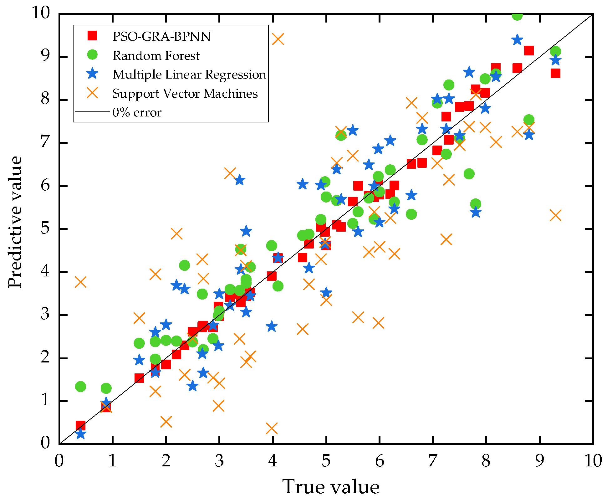
The PSO-GRA-BPNN established in this paper is compared with the traditional BP neural network, multiple linear regression, random forest [12], and support vector machine regression models [30], and the advantages of the prediction accuracy of this model are verified by actual cases, which provides a new idea and method for used car evaluation.

2. Data and Model Assumptions

2.1. Analysis of Elements Making the Price of Used Cars Different

As a commodity, a used car not only has its attributes that will affect the price, but also some external factors will also affect the value of the used car. Factors affecting the value of used cars should be fully considered, as well as the availability of indicator data. This paper will analyze the factors of the vehicle itself and the market and analyze the factors that affect the price of used cars in combination with the parameters of used cars, vehicle condition factors, and transaction factors [31,32,33].

Vehicle parameters refer to the characteristics of the car itself, mainly including the brand and vehicle configuration. Due to the different brands of vehicles, there will be differences in the configuration of the vehicle’s gearbox, body structure, etc., and there will be differences in the prices of different vehicle brands due to differences in manufacturing costs. Vehicle configuration is mainly reflected in the functional attributes of the car, including driving mode, gearbox type, engine power, body structure, and other parameters. Different functional configuration methods have differences in the price of used cars.

The vehicle condition factors mainly refer to the vehicle condition after the used car is used, which can be divided into depreciation factors and environmental factors. The miles and usage period of a used car account for the majority of the depreciation element. The longer the vehicle is used or the longer the mileage, the greater the wear and tear of the vehicle and the lower the value of the second-hand car. Environmental factors refer to the vehicle’s displacement, fuel consumption, and emission standards. Since oil prices are the focus of second-hand car buyers, small-displacement vehicles are more fuel-efficient and low-fuel-consumption vehicles have high-value retention rates, which are more preferred by consumers.

Transaction factors mainly refer to the impact of the external environment, including regions and new car prices. Due to the different emission standards in each region, the circulation restricts the used car to only be circulated locally. Buying a second-hand car in another place will encounter the situation of being unable to transfer the ownership, which will directly affect the value-preserving rate of the second-hand car. The cost of used automobiles is directly linked to the cost of new cars, and the cost of new cars can influence the cost of used cars. In general, the more expensive a new car is, the more expensive a used car is.

Therefore, 12 characteristic variables including brand, drive mode, gearbox type, engine power, body structure, mileage, usage time, displacement, fuel consumption, emission standard, region, and new car price are selected as the influencing factors of the used car price.

2.2. Data Selection and Processing

This article obtains a total of 10,260 used car data in East China from a used car trading platform, and the data come from https://www.iautos.cn/ (accessed on 24 March 2022). As China’s leading online used car trading market, the used car trading platform has authentic and reliable transactions and a wide range of business coverage, providing real data for evaluation. As seen in the following table, each piece of data has 12 distinctive variables.

Table 1. The 12 distinctive variables.

Variable	Definition	Variable	Definition
x1	Brand	x7	Usage time
x2	Drive mode	x8	Displacement
x3	Gearbox	x9	Fuel consumption
x4	Engine power	x10	Emission standard
x5	Body structure	x11	Region
x6	Mileage	x12	New car price

describes the 12 distinctive variables in detail.

Next, we preprocess the data in the following ways:

(1)

For data columns that can be calculated quantitatively, such as displacement and new car price, use Lagrange interpolation to calculate their missing values, and delete missing values that are difficult to quantify such as brand and region.

(2)

According to the ranking of “100 Most Valuable Auto Brands in the World in 2021” released by Brand Finance, different brands are coded and digitized.

(3)

There are three driving modes: front-wheel drive, rear-wheel drive, and four-wheel drive, which are denoted by the numbers 0, 1, and 2.

(4)

The gearbox is divided into two types: automatic and manual, and it is converted into a Boolean type, that is, the number of automatic is 0, and the number of manual is 1.

(5)

The body structure is divided into the single box, hatchback, and sedan, delete a few single boxes, convert the hatchback to number 0, and the sedan to number 1.

(6)

The usage time is converted to the number of days since the data were acquired.

(7)

Since the National III cars are gradually being phased out, a small number of National III cars are deleted, and National IV is converted to the number 4, National V is converted to the number 5, and National VI is converted to the number 6.

(8)

The value is assigned according to the number of prefecture level cities in different provinces. Anhui Province is assigned 1–17, Zhejiang Province is assigned 18–28, Fujian Province is assigned 29–38, Jiangxi Province is assigned 39–51, Jiangsu Province is assigned 52–65, Shandong Province is assigned 66–81, and Shanghai is assigned 82.

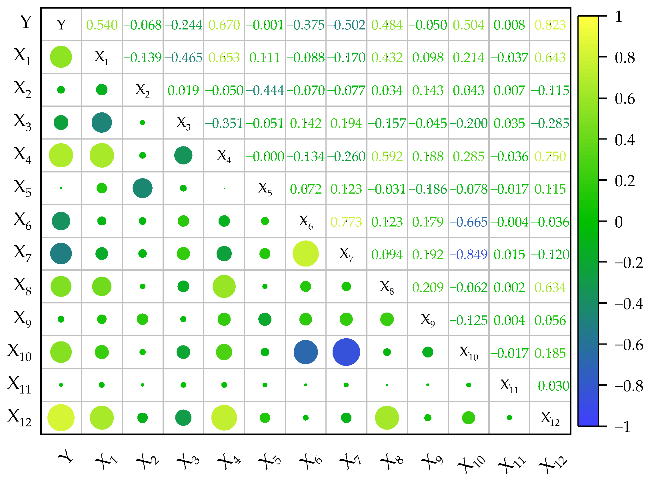
2.3. Analysis of Pearson Correlation

The Pearson correlation analysis was used to quantitatively describe the degree of linear correlation among various parameters to study the linear correlation between the influencing factors of used car prices [34,35], and the Pearson correlation matrix was calculated based on the obtained data, as shown in Figure 1.

In Figure 1, the closer the absolute value of the Pearson correlation coefficient r (X, Y) is to one, the stronger the linear correlation between the two indicators, and the closer the absolute value is to zero, the weaker the correlation. In addition, when r (X, Y) is positive, the two are positively correlated; when r (X, Y) is negative, the two are negatively correlated. It is clearly stated that only the correlation coefficient between new car price, engine power, and used car price is greater than 0.6, which has a certain linear correlation. Therefore, nonlinear modeling methods are advised preferably to conduct market forecast.

2.4. Assumptions

To ensure the rigor of the experiment, the following assumptions should be presented:

(1)

Since the collected data are not the data after the actual transaction on the platform, we assume that every used car on the platform can be successfully traded at the page price.

(2)

The price of used cars is not only affected by their internal configuration but also by the external environment. We assume that the price of used car pages provided by the platform will not be affected by the external environment.

3. Methodology

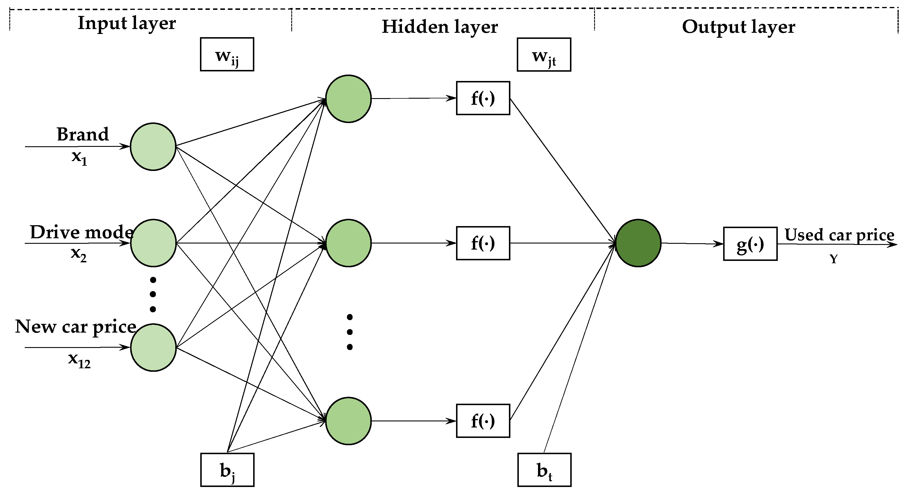
3.1. BP Neural Network

A complete BP neural network model usually includes three basic network structures: input layer, hidden layer and output layer, and each layer can contain multiple neurons. Generally speaking, the number of neurons in the input layer and output layer is equal to the input and output vector dimensions of the sample data, so the structure of the BP neural network is generally determined by the hidden layer. The hidden layer can have a single layer or multiple layers. In theory, a single hidden-layer neural network can approximate a nonlinear function with arbitrary precision, thereby realizing a nonlinear mapping from input to output. The network error can be minimized, and the accuracy can be increased by adding hidden layers; however, this complicates the network, increases the training time, and increases the likelihood of overfitting. Therefore, the single-hidden-layer neural network is given priority to obtain lower errors at a lower cost of increasing hidden-layer nodes [36].

BPNN includes two processes during operation: the forward transfer of the signal combined with the reverse of the error [37,38,39,40]. The network forwardly transmits the external information as the input signal and passes it to the output layer through the hidden-layer calculation. During this procedure, the calculation will be performed according to the given initial weights and thresholds, and then the outputs will be finally realized. If there is an error between the output layer output and the expected output, back propagation is entered. The error signal continuously adjusts the connection weights and thresholds from the output layer through the hidden layer forward layer by layer, so that the predicted output of the network is close to the expected output. The cycle repeats until the error is reduced to a predetermined accuracy.

Figure 2 depicts the BPNN structure employed in this work.

Take the 12 variables that affect the price of used cars as the input vector X = (x₁, x₂, …, x₁₂) and the used car price Y = (y) as the output vector and provide them to the established neural network; then, each unit’s output value $Z_j$ in the hidden layer is:

$$Z_j=f\left(\sum _{\mathrm{i}=1}^{\mathrm{n}}\left({\mathrm{w}}_{\mathrm{ij}}{\mathrm{x}}_{\mathrm{i}}-{\mathrm{b}}_{\mathrm{j}}\right)\right)$$

(1)

In the above equation, $w_{ij}$ and $b_j$ are the connection weight and threshold between the input layer and the hidden layer; i is the dimension of the input layer, and i = 1, 2, 3, …, n; j denotes the dimension of the hidden layer, and j = 1, 2, 3, …, m; f represents the hidden-layer activation function.

Similarly, to determine the output $O_t$ of each unit in the output layer, the connection weight $w_{jt}$ and threshold $b_{\mathrm{t}}$ from the hidden layer and the output counterpart are used.

$$O_t=g\left({\displaystyle {\sum }_{j=1}^m\left(w_{jt}{Z}_j-b_t\right)}\right)=g\left({\displaystyle {\sum }_{j=1}^m\left(w_{ij}f\left({\displaystyle {\sum }_{i=1}^n\left(w_{ji}{x}_i-b_j\right)}\right)-b_t\right)}\right)$$

(2)

In the above equation, t represents the dimension of the output layer, and j = 1, 2, 3, …, m; g represents the activation function of the output layer.

Therefore, the sum of squared errors $E$ between the network output vector O and the used car price Y is

$$E=\frac{1}{2}{{\displaystyle {\sum }_{t=1}^l\left(y_t-O_t\right)}}^2$$

(3)

Step by step, extend back to the hidden layer and the input one, obtaining:

$$E=\frac{1}{2}{\displaystyle {\sum }_{t=1}^l{\left(y_t-g^{\prime }\left({\displaystyle {\sum }_{j=1}^m\left(w_{jt}{Z}_j-b_t\right)}\right)\right)}^2}$$

(4)

$$E=\frac{1}{2}{{\displaystyle {\sum }_{t=1}^l\left(y_i-g^{\prime }\left({\displaystyle {\sum }_{j=1}^m\left(w_{ji}{f}^{\prime }\left({\displaystyle {\sum }_{i=1}^n\left(w_{ij}{x}_i-b_j\right)}\right)-b_t\right)}\right)\right)}}^2$$

(5)

In the above equation,$f^{\prime }$ and $g^{\prime }$ represent the inverse of activation functions f and g, respectively.

Based on the minimum error, the gradient descent method and iterative solution are involved. Gradually correcting the connection weights and thresholds between the input layer and the hidden layer and the hidden layer and the output layer, the neural network’s final output is finally approaching the values that were anticipated in order to achieve perfection for the error squared sum E.

3.2. BPNN Prediction Model Based on GRA Variable Screening

When investigating a multivariate complex system, qualitative analysis methods are typically employed to screen out independent factors that have a large impact on the dependent variables, and then a system model is built. Given a large number of independent variables present, using them as BPNN input variables will raise the network’s complexity, diminish its performance, lengthen the computation time, and impact prediction accuracy.

GRA provides a better way to solve this problem [41,42,43,44,45]. It analyzes the geometric similarity from the dependent variable sequence to the independent one to determine the connection between different independent variable sequences and dependent variables. If the geometric shapes between the sequences are similar, the degree of association is strong and vice versa. In this method, we utilize GRA to filter out the independent variables that have a vital effect on the dependent variable as input nodes, and then we use the BPNN algorithm to train. Only by doing so can the BPNN algorithm strengthen multivariate complex system modeling ability. The general steps of GRA are as follows:

• Step 1: Determine the analysis index system and collect analysis data. Let m data sequences form the following matrix:

$$\left(X_1^{\prime },X_2^{\prime }\cdots ,X_m^{\prime }\right)=\left(\begin{array}{cccc}{x}_1^{\prime }(1)& x_2^{\prime }(1)& \cdots & x_m^{\prime }(1)\\ x_1^{\prime }(2)& x_2^{\prime }(2)& \cdots & x_m^{\prime }(2)\\ ⋮& ⋮& ⋮& ⋮\\ x_1^{\prime }(n)& x_2^{\prime }(n)& \cdots & x_m^{\prime }(n)\end{array}\right)$$

(6)

In the formula, n is the number of indicators, $X_i^{\prime }={\left(x_i^{\prime }(1),x_i^{\prime }(2),\dots x_i^{\prime }(n)\right)}^T$, i = 1, 2, …, m.

• Step 2: Determine the reference and comparison sequences in the system.

The reference sequence is considered to be the sequence that reflects the behavioral characteristics of the system, and the comparison sequence is considered to be the sequence that affects the behavioral characteristics of the system.

$$\mathrm{Reference}\mathrm{sequence}:X_0^{\prime }=\left(x_0^{\prime }(1),x_0^{\prime }(2),\cdots ,x_0^{\prime }(n)\right)$$

(7)

$$\mathrm{Comparison}\mathrm{sequence}:X_i^{\prime }=\left(x_i^{\prime }(1),x_i^{\prime }(2),\cdots ,x_i^{\prime }(n)\right)$$

(8)

• Step 3: Apply dimensionless processing to the dependent and independent variable sequences, using the mean value processing approach described below.

$$X_I=X_l^{\prime }/\overline{X_l^{\prime }}=\left(x_i(1),x_i(2),\cdots ,x_i(n)\right)$$

(9)

The dimensionless data sequence forms the following matrix:

$$\left(X_0,X_1,\cdots ,X_m\right)=\left(\begin{array}{cccc}{x}_0(1)& x_1(1)& \cdots & x_m(1)\\ x_0(2)& x_1(2)& \cdots & x_m(2)\\ ⋮& ⋮& ⋮& ⋮\\ x_0(n)& x_1(n)& \cdots & x_m(n)\end{array}\right)$$

(10)

• Step 4: Calculate the absolute difference between each compared sequence and the corresponding element of the reference sequence in turn.

$$\Delta =\left|x_0(k)-x_i(k)\right|$$

(11)

In the formula, k = 1, 2, …, n.

• Step 5: Calculate the correlation coefficient between the compared sequence and the corresponding factor in the reference sequence.

$$\xi \left(x_0(k),x_i(k)\right)=\frac{\underset{i}{\min }\underset{k}{\min }|x_0(k)-x_i(k)|+\rho \underset{i}{\max }\underset{k}{\max }|x_0(k)-x_i(k)|}{|x_0(k)-x_i(k)|+\rho \underset{i}{\max }\underset{k}{\max }|x_0(k)-x_i(k)|}$$

(12)

In the above equation, $\rho$ represents the resolution coefficient, which reflects the size of the discrimination. The value ranges from 0 to 1 and is usually taken as 0.5.

• Step 6: Calculate the degree of association and sort the degree of association to obtain the relative closeness of each comparison sequence and the reference sequence.

$$r\left(X_0,X_i\right)=\frac{1}{n}\sum _{k=1}^n\xi \left(x_0(k),x_i(k)\right)$$

(13)

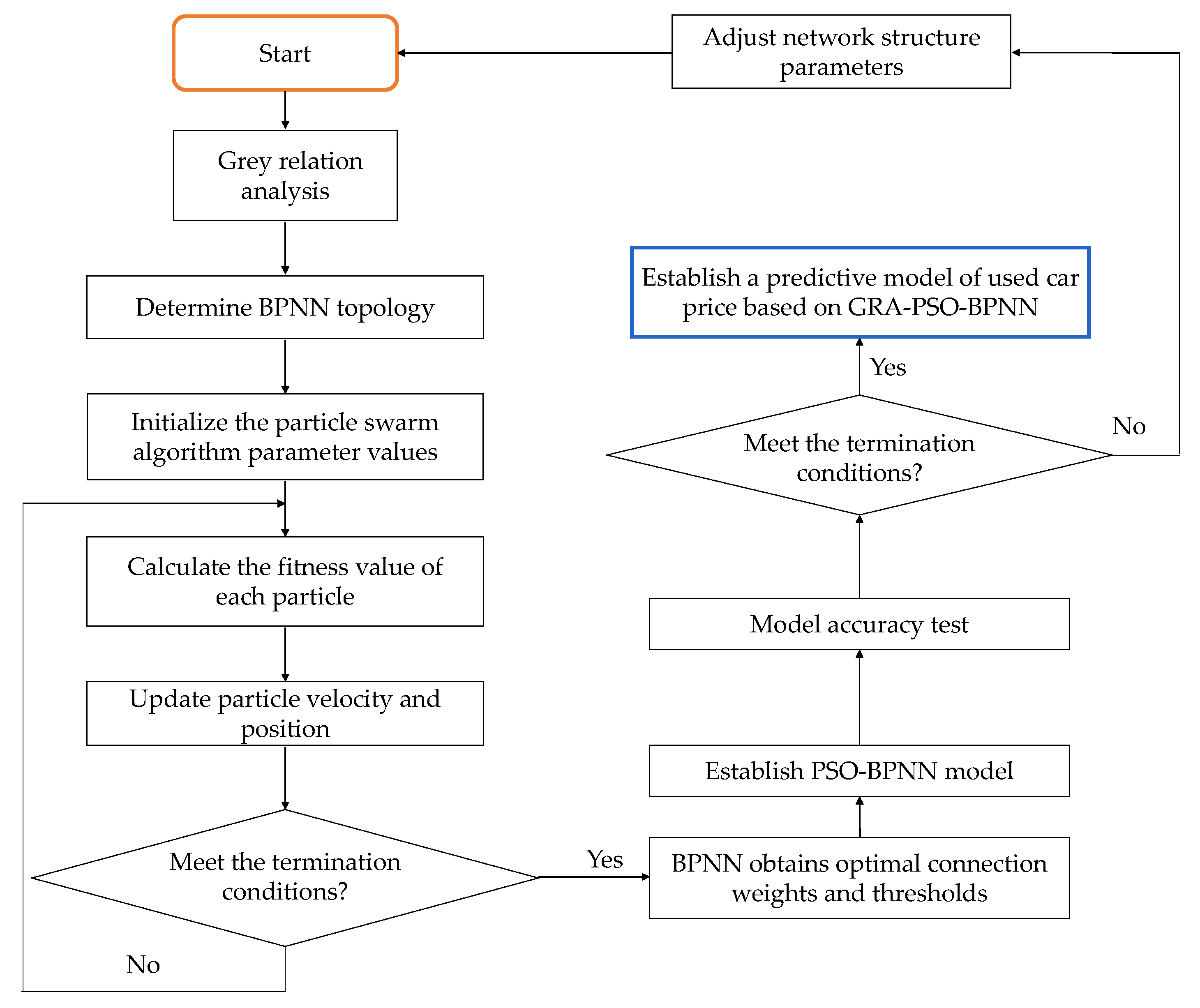
3.3. Construction of GRA-BPNN Prediction Model Based on PSO Optimization Algorithm

There is a significant difference between the actual value and the predicted value when a single BPNN model is used to generate a prediction. In fact, the network has a slow convergence speed, and even with a few training samples, it is impossible to avoid slipping into the trap of local optimum. An overfitting problem may occur too. Particle swarm optimization (PSO) is known for its ease of use, quick convergence, and good global optimization. PSO is recommended in this approach to polish the BPNN model.

Unlike other evolutionary algorithms, such as genetic algorithms, the PSO algorithm treats each individual as a single particle with no mass and volume flying at a specific speed and direction, and each particle is a potential solution to the actual problem, so particles are optimized in an N-dimensional search space [46,47,48,49,50].

The current fitness value is computed by the fitness function established in advance, and the ith particle’s position in the N-dimensional search space is $z_i=\left(z_{i1},z_{i2},\cdots ,v_{in},\cdots ,z_{iN}\right)$, the current fitness value is calculated by the fitness function set in advance, and $v_i=\left(v_{i1},v_{i2},\cdots ,v_{id},\cdots ,v_{iD}\right)$ shows the speed at which the particle is flying. In each iteration process, the particle finds the optimal solution by moving to two optimal positions. One is the particle found so far, which is called the local optimal pbest; the other is the optimal identified by the whole population so far, that is, the global optimal gbest. The particle swarm will store the individual and the global optimums amid the optimization process.

Additionally, by updating its speed and position settings using the Equations (14) and (15), one can discover the best solution to the optimization problem.

$$v_i=\omega \times v_i+c_1\times r+\left(pbest-z_i\right)+c_2\times r\times \left(gbest-z_i\right)$$

(14)

$$z_i=z_i+v_i$$

(15)

In the above two formulas, i = 1, 2, 3, …, n signifies the total of particle swarms; v_i is the speed of particles; $\omega$ represents the inertia factor; c₁, c₂ represent the learning factor; pbest represents the individual optimal solution; gbest represents the overall optimal solution; r represents a random constant between 0–1; z_i means the particle position.

The particle speed has an impact on the optimization ability of the algorithm. Too fast speed may cause the particles to cross the optimal position, and too slow speed will make it unable to completely optimize in the population space. Therefore, it is necessary to limit the speed of particle flight. By setting the maximum value v_max and minimum value v_min of the speed, the value range of the corresponding setting position is z_min-z_max.

To train the initial parameters of BPNN using the PSO algorithm, express all existing connection weights and thresholds in BPNN as specific individuals, map these individuals one-to-one to the particles in the PSO algorithm, and calculate the fitness of each particle using the particles’ fitness function. The training error of the BPNN is the fitness. In each iteration, compare the size of the individual extreme with the size of the group extreme and obtain the global optimal value, that is, the best initial weight and threshold in the BPNN, using the continuous update of particle velocity and position.

• Step 1: Define the PSO-GRA-BPNN model’s inputs and outputs.

The characteristic variables that affect the price of used cars are screened through grey relational analysis as the input of the network, and the price of used cars is used as the output.

• Step 2: Particle swarm initialization.

Initially, a specified number of particle swarms are randomly generated, the number of particles n is determined, each particle is initialized, the particle’s initial position and velocity are randomly generated, and the maximum number of iterations and termination conditions are confirmed. The search dimension N of the vector group is confirmed by the total of thresholds and weights to be optimized in the BPNN structure:

$$\mathrm{N}=\mathrm{y}+\mathrm{l}+\mathrm{x}\times \mathrm{l}+\mathrm{y}\times \mathrm{l}$$

(16)

• Step 3: Calculate a single particle’s fitness value.

The particle’s fitness value is computed using the fitness function. The particle swarm’s fitness value is inversely proportional to its fitness value.

$$F=\frac{1}{S}\left({\displaystyle {\sum }_{K=1}^S{\displaystyle {\sum }_{I=1}^N\left(y_{ki}-{y^{\prime }}_{ki}\right)}}\right)$$

(17)

In the above equation, S is the number of samples; N represents the dimension of the space where the particle swarm is located; $y_{ki}$ represents the prediction of the neural network output value; $y_{ki}^{\prime }$ denotes the expected output value of the neural network.

• Step 4: Update particle velocity and position.

The fitness value of each particle is compared with the fitness value of the group’s ideal location, and the optimal position is chosen as the optimum of the population at this moment. According to Equations (14) and (15), the particle swarm velocity and position are renovated.

• Step 5: Optimal particle count.

The procedure finishes when the population iteration error reaches the setting accuracy E, and the global optimal solution may be found and projected to the BP network’s weights and thresholds.

• Step 6: PSO-GRA-BPNN model training.

Input the training data to train the PSO-GRA-BPNN model after determining the PSO-GRA-BPNN weights and thresholds. The comprehensive representation of the whole flow chart is shown in Figure 3.

4. Results

4.1. Model Evaluation Metrics

There are many methods for evaluating the model predictions. In the following, four indicators, the average relative error MAPE, the average absolute error MAE, and the correlation coefficient R combined with the goodness-of-fit R², are conducted predict to the model accuracy. The evaluation functions are:

$$\mathrm{MAPE}=\frac{100\%}{n}\times \sum _{t=1}^n\left|\frac{y_t-{\widehat{y}}_t}{y_t}\right|$$

(18)

$$MAE=\frac{1}{n}\sum _{t=1}^n\left|y_t-{\widehat{y}}_t\right|$$

(19)

$$R=\frac{{\displaystyle \sum _{t=1}^n}\left({\widehat{y}}_t-\overline{{\widehat{y}}_t}\right)\left(y_t-{\overline{y}}_t\right)}{\sqrt{{\displaystyle \sum _{t=1}^n}{\left({\widehat{y}}_t-\overline{{\widehat{y}}_t}\right)}^2}\sqrt{{\displaystyle \sum _{t=1}^n}{\left(y_t-{\overline{y}}_t\right)}^2}}$$

(20)

$$R^2=1-\frac{{\displaystyle \sum _{t=1}^n{(y_t-{\widehat{y}}_t)}^2}}{{\displaystyle \sum _{t=1}^n{(y_t-{\overline{y}}_t)}^2}}$$

(21)

In the above equations, ${\widehat{y}}_t$ denotes the predicted value of the used car, ${\mathrm{y}}_{\mathrm{t}}$ stands for the actual value of the used car, $\overline{{\widehat{y}}_t}$ is the average of the predicted value of the used car, and ${\overline{y}}_t$ demonstrates the average value of the actual value of the used car.

4.2. Model Building Process

Guaranteeing the completeness of the prediction, we use the normalization to process the input data preceding training.

$${\mathrm{X}}^{*}=\frac{\mathrm{X}-\mathrm{MAX}}{\mathrm{MAX}-\mathrm{MIN}}$$

(22)

In the above equation, $X^{*}$ represents the result after transformation, X stands for the original, MIN represents the minimum value of the column where the data is located, and finally, MAX represents the maximum value of the column where the data is located.

4.2.1. BPNN Prediction Model

There are 7702 pieces of test data processed in this paper. The neural network prediction set T is chosen as the first 6702 sets of data, which is utilized to finish the model’s development, and the test set T_test is chosen as the final 1000 items of data, testing the prediction effect of the constructed model.

The Levenberg–Marquart method is used to train the BPNN, and the tansig and purelin functions are used to activate the hidden and output layers, respectively. According to the empirical formula, the number of neurons in the hidden layer can be Figured out with $l$:

$$l=\sqrt{x+y}+a$$

(23)

In the above equation, l is the number of nodes in the hidden layer; x symbolizes the number of nodes in the input layer; y denotes the number of nodes in the output counterpart; and a is a constant ranging from 1 to 10.

Substitute x = 12, y = 1 into Equation (23) to obtain $l$= 4~14. Figuring out the optimal value belonging to the hidden-layer node $l$, 11 node values in the range of $l$ = 4 to 14 are used to train BPNN, and the training results are compared, as shown in

Table 2. Prediction effects of different hidden-layer nodes.

Neurons in the Hidden Layer	MAPE	MAE	Training Speed	Number of Network Iterations
$l$ = 4	30.914%	0.671	0.419 s	13
$l$ = 5	32.873%	1.256	1.103 s	48
$l$ = 6	28.245%	0.753	0.714 s	24
$l$ = 7	51.237%	1.493	0.542 s	16
$l$ = 8	38.634%	0.957	1.906 s	62
$l$ = 9	43.670%	1.374	1.788 s	57
$l$ = 10	9.891%	0.585	1.868 s	54
$l$ = 11	13.934%	0.816	2.261 s	55
$l$ = 12	27.836%	1.073	0.751 s	14
$l$ = 13	20.897%	1.016	1.714 s	40
$l$ = 14	45.383%	0.924	1.324 s	17

.

According to Table 2, the MAPE and MAE of the model are the lowest, with values of 9.891 and 0.585%, respectively, indicating that when the number of hidden layers is 10, the accuracy of the model is the highest. In terms of training time, when the number of hidden layers is 10, the training time is longer, but 0.363 s is saved compared with the longest training time. From the performance of the model, the number of hidden layers selected in this paper is 10, which sacrifices time for higher accuracy, and the number of network iterations is 54. A 12-10-1 three-tier BPNN used car price prediction model is constructed. The target error is 0.00001, and the learning rate is 0.01.

4.2.2. GRA-BPNN Prediction Model

On the basis of the BPNN, GRA is used for variable screening. The 12 variables that affect the price of used cars are used as the comparison sequence, and the price of used cars is used as the reference sequence to calculate the gray correlation between the sequences. The results are shown in

Table 3. Calculation results of grey relational degree.

Variable	Correlation	Ranking	Variable	Correlation	Ranking
x12	0.913	1	x2	0.595	7
x8	0.861	2	x11	0.591	8
x6	0.819	3	x4	0.589	9
x3	0.775	4	x10	0.578	10
x9	0.733	5	x5	0.497	11
x7	0.720	6	x1	0.472	12

.

The above analysis demonstrates that the correlation of new car price x₁₂, displacement x₈, mileage x₆, gearbox x₃, fuel consumption x₉, and registration time x₇ are all greater than 0.7, while the correlation degree of drive mode x₂, region x₁₁, engine power x₄, emission standard x₁₀, body structure x₅, and brand x₁ are less than 0.7. GRA is able to identify key factors affecting used car prices and provide more efficient inputs to predictive models. Therefore, choose the new car price, displacement, mileage, gearbox, fuel consumption, and registration time as the network input of the BPNN, set the same parameters and functions as the above BPNN, and construct a 6-10-1 three-layer structure GRA-BPNN used car price prediction model.

4.2.3. PSO-GRA-BPNN Prediction Model

Take the new car price, displacement, mileage, gearbox, fuel consumption, and registration time as the network input of PSO-GRA-BP and the used car price as the network output. Using the same number of hidden layers and functions as GRA-BPNN, a 6-12-1 three-layer structure PSO-GRA-BPNN used car price prediction model is constructed. The main parameters involved in particle swarm optimization are learning factors c₁ and c₂, maximum speed V_max, inertia weight ω, population size N, and number of iterations. The settings of the parameters are as follows [51,52,53,54]:

(1)

The learning factors c₁ and c₂: c₁ and c₂ are mainly the adjustment weights of particles that affect their own and group experience. If the value of c₁ is zero, the particles only have group experience, and local convergence may occur; if the value of c₂ is zero, information sharing cannot be carried out in the group, and you only have your own experience. If both are zero, particles cannot effectively obtain empirical information, and the motion of particle swarm will show a chaotic state. Therefore, the values of c₁ and c₂ can have a great impact on the whole model. In this paper, the values of c₁ and c₂ are taken as 1.49445.

(2)

The maximum speed V_max: During the effective search process of particles, the velocity of particle motion is usually described by V_max, and the search step size of particles is adjusted. When the value of V_max is too large, the position of the particle may exceed the optimal position; when the value of V_max is too small, the particle may have a problem of slow convergence. In this paper, V_max is chosen to be one.

(3)

The inertia weight ω: The inertia weight ω will have a significant impact on the convergence of the particle swarm optimization algorithm. If ω is relatively small, the local search ability of the particle swarm optimization algorithm is strong, but the global search ability is low; if ω is large, the opposite characteristics are exhibited. Therefore, this paper selects the inertia weight as 0.9.

(4)

Population size N: Too small of a population size will lead to insufficient accuracy and will be extremely unstable, and too large of a population size will lead to performance degradation. For higher accuracy and stability, this paper takes n as 200.

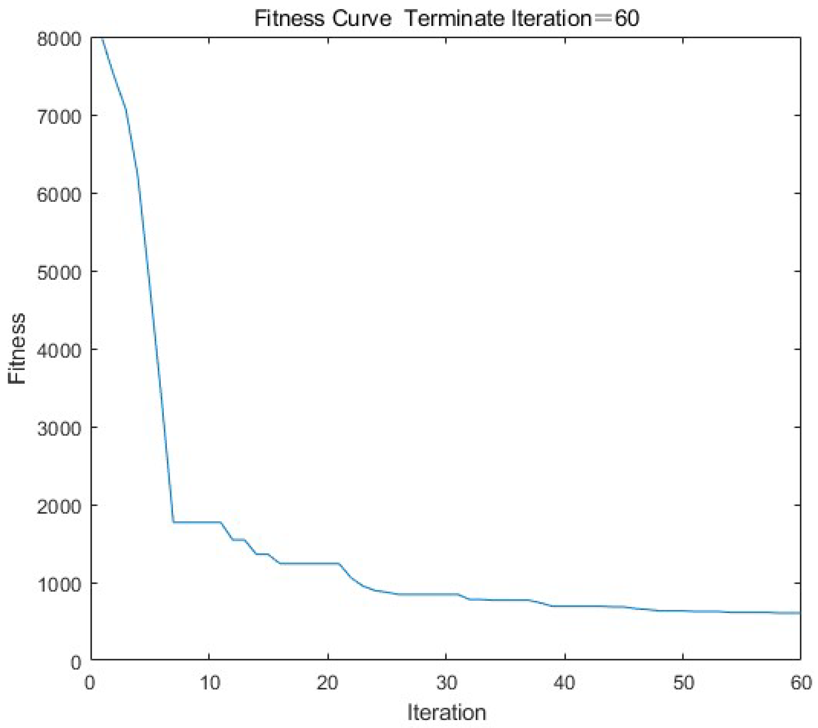
(5)

Number of iterations: As can be seen from the Figure 4 below, the change trend of the error between the expected value and the absolute value of the actual output is that with the number of iterations from 0 to 20, and the overall error of the model decreases significantly. When the number of iterations is from 20 to 60, the slope of the curve tends to be zero, and the error of the model no longer decreases. If you continue to increase the number of iterations of the model, it will consume a lot of time resources, and the performance of the model will not be well-improved. Therefore, set the number of iterations to 60.

4.3. Models Comparison

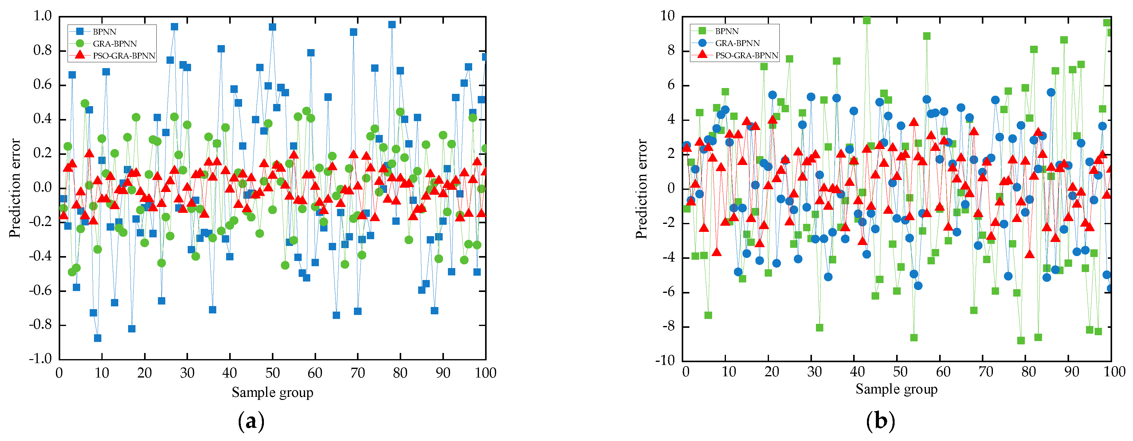
4.3.1. Comparison of Results of Different BPNN Prediction Models

For the three BPNN models established above, (1) is the BPNN prediction model, (2) is the GRA-BPNN prediction model after featuring variable screening, and (3) is the PSO-GRA-BPNN model after featuring variable screening combined with PSO method, respectively. For the comparison of used car price prediction effects, the results turned out as follows (

Table 4. Comparison of BPNN prediction models.

Model	MAPE	MAE	R	R2	Training Speed
BPNN	9.891%	0.585	0.991	0.912	12.549 s
GRA-BPNN	7.118%	0.529	0.995	0.969	6.506 s
PSO-GRA-BPNN	3.936%	0.475	0.998	0.984	94.153 s

).

The three models were evaluated based on the five indicators mentioned above:

(1)

MAPE can more correctly depict the percentage difference between anticipated and true values, and the lower its value, the better the fitting effect. From the above table, we can see that the MAPE of PSO-GRA-BPNN is the smallest, GRA-BPNN is the second, and BPNN is the largest. This indicates that PSO-GRA-BPNN has high prediction accuracy.

(2)

MAE is the sum of the absolute values of the difference between the predicted value and the actual value. It measures the closeness of the predicted result to the actual dataset. The smaller the value and the closer to zero, the better the fitting effect. The MAE of PSO-GRA-BPNN is the smallest, and its value is 0.475, which indicates that the deviation of the predicted value of PSO-GRA-BPNN from the actual value is the smallest, and the actual prediction error value is the smallest.

(3)

R is between zero and one. The closer it is to one, the better the model’s prediction, and the closer it is to zero, the worse the model’s prediction. R is the smallest for BPNN with a value of 0.991, followed by GRA-BPNN with a value of 0.995, and the largest for PSO-GRA-BPNN with a value of 0.998. This indicates that the predicted value of PSO-GRA-BPNN has the strongest correlation with the true value.

(4)

R² is the goodness of fit, and the closer the value of the coefficient of determination is to one, the better the regression is. From the table, we can see that PSO-GRA-BPNN has the largest R² value, 0.984, which is the best goodness of fit among these three models.

(5)

From the training speed, it can be seen that PSO-GRA-BPNN has the slowest training speed with a time of 94.153 s, and GRA-BPNN has the fastest training speed with a time of 6.506 s. Using the GRA method can effectively shorten the running time of the model, but adding the PSO method increases the running time, although the prediction accuracy of PSO-GRA-BPNN is higher than that of BPNN and GRA-BPNN, and the time is lost.

In the sample data, the distribution of used car prices is extremely uneven, with 55% of used cars costing CNY 0–200,000, 38.5% of used cars costing CNY 200,000–400,000, and CNY 400–600,000 used cars accounting for 38.5%. In total, 5.3 and 1.2% of used cars are over CNY 600,000. Therefore, a used car with a value of CNY 0–200,000 is defined as a low-priced used car, and a used car with a value of more than CNY 200,000 is defined as a high-priced used car. The prediction error graphs are as follows (Figure 5).

As seen in the graph above, the three models are more accurate at predicting the price of low-priced used automobiles than high-priced used cars. Furthermore, whether it is a low-priced or high-priced used automobile, the PSO-GRA-BPNN model performs better than the BPNN and GRA-BPNN models in terms of prediction accuracy.

4.3.2. Comparison with Other Used Car Price Prediction Models

Currently, the used car price prediction models established by researchers can be divided into three categories: the random forest model, the multiple linear regression model, and the support vector machines regression model.

Table 5. Comparison with other investigators’ predictive models.

Model	MAPE	MAE	R	R2	Training Speed
PSO-GRA-BPNN	3.936%	0.475	0.998	0.984	94.153 s
Random Forest	19.933%	0.842	0.664	0.553	20.810 s
Multiple Linear Regression	33.977%	1.097	0.949	0.917	1.914 s
Support Vector Machines	153.958%	0.028	0.943	0.863	0.057 s

and Figure 6 demonstrate the outcomes of these two forms of used car price prediction implemented in Python.

It can be seen from Table 5 that the prediction accuracy of the PSO-GRA-BPNN model for used car prices is significantly higher than that of the other three types of prediction models. MAPE is the lowest, with a maximum reduction of 150.022%; MAE is the lowest, with a maximum reduction of 0.622; R and R² are the highest, but the training speed is the longest. At the same time, it can be seen from Figure 6 that most of the prediction points of the random forest model and the multiple regression model are above the 0% error bar, and the overall prediction value is high; the support vector machine regression model prediction points are more evenly distributed on both sides of the 0% error bar, but the overall deviation is large.

In summary, in the process of predicting used car prices, the PSO-GRA-BPNN model has the longest training time and the PSO-GRA-BPNN model has the lowest MAPE and MAE and R and R² are the highest. The overall prediction effect is significantly better than the multiple linear regression model, random forest models, and support vector machine regression model.

5. Conclusions

In recent years, online used car trading platforms have developed rapidly, but they still face many problems. In practice, institutions and individuals differ in how they screen the characteristic variables of used car prices and predict used car prices. Under such conditions, it is easy to lead to the unsound development of the market, and it is difficult to establish a unified evaluation system, which causes great difficulties in the transaction of used cars. In terms of theory, traditional used car price evaluation methods rely too much on the subjective judgment of evaluators, which can no longer meet the needs of online transactions in the used car market. Therefore, it is necessary to establish an efficient, reasonable, fair, and accurate used car price evaluation system.

This paper analyzes the factors affecting the price of used cars from three aspects—used car parameters, vehicle condition factors, and transaction factors—and establishes a used car price evaluation system including 12 characteristic variables. Using web crawler technology to obtain used car transaction data, three prediction models of BPNN, GRA-BPNN, and PSO-GRA-BPNN were constructed to conduct comparative verification and result analysis. In a rough comparison, the BPNN model has lower accuracy, with an error range of about 19.979%, and it is unstable. In the case of feature variable screening, the prediction accuracy of the GRA-BPNN model is higher than that of the BPNN, and the error range is about 13.986%. However, the constructed PSO-GRA-BPNN used car price prediction model not only has high accuracy but also has an error range of about 7.978%, which has good scalability.

Although the PSO-GRA-BPNN used car price prediction model has high prediction accuracy, it has lost time. It is mainly analyzed from two aspects. First, when selecting the hidden layers of the BP neural network, accuracy is given priority and time is ignored. The second is to select the iteration number and population size of the particle swarm optimization algorithm. When the iteration number and population size are larger, the accuracy of the model is higher, but with the continuous increase of the value, the improved accuracy is very small, almost stable. In addition, in view of the fact that the prediction accuracy of high-end used cars is lower than that of low-end used cars, it is suggested that when pricing high-end used cars, you need to check other configuration information in order to make a more reasonable judgment.

References

1. Ticknor, J.L. A Bayesian regularized artificial neural network for stock market forecasting. Expert Syst. Appl. 2013, 40, 5501–5506. [Google Scholar] [CrossRef]
2. Livieris, I.E.; Pinteals, E.; Pintelas, P. A CNN-LSTM model for gold price time-series forecasting. Neural Comput. Appl. 2020, 32, 17351–17360. [Google Scholar] [CrossRef]
3. Dou, Z.-W.; Ji, M.-X.; Wang, M.; Shao, Y.-N. Price prediction of Pu’er tea based on ARIMA and BP models. Neural Comput. Appl. 2021, 34, 3495–3511. [Google Scholar] [CrossRef]
4. Mehmet, Ö. Predicting second-hand car sales price using decision trees and genetic algorithms. Alphanumeric J. 2017, 5, 103–114. [Google Scholar]
5. Dimoka, A.; Hong, Y.-L.; Pavlou, P.A. On product uncertainty in online markets: Theory and evidence. Mis Quart. 2012, 36, 395–426. [Google Scholar] [CrossRef] [Green Version]
6. Xu, M.; Tang, W.-S.; Zhou, C. Operation strategy under additional service and refurbishing effort in online second-hand market. J. Clean. Prob. 2021, 290, 125608. [Google Scholar] [CrossRef]
7. Shafiee, M.; Chukova, S. Optimal upgrade strategy, warranty policy and sale price for second-hand products. Appl. Stoch. Models Bus. Ind. 2013, 29, 157–169. [Google Scholar] [CrossRef]
8. Kwak, M.; Kim, H.; Thurston, D. Formulating second-hand market value as a function of product specifications, age, and conditions. J. Mech Design. 2012, 134, 032001. [Google Scholar] [CrossRef]
9. Fathalla, A.; Salah, A.; Li, K.-L.; Li, K.-Q.; Francesco, P. Deep end-to-end learning for price prediction of second-hand items. Knowl. Inf. Syst. 2020, 62, 4541–4568. [Google Scholar] [CrossRef]
10. Stefan, L.; Stefan, V. Car resale price forecasting: The impact of regression method, private information, and heterogeneity on forecast accuracy. Int. J. Forecasting 2017, 33, 864–877. [Google Scholar]
11. Tan, Z.-P.; Cai, Y.; Wang, Y.-D.; Mao, P. Research on the Value Evaluation of Used Pure Electric Car Based on the Replacement Cost Method. In Proceedings of the 5th International Conference on Mechanical Engineering, Materials Science and Civil Engineering (ICMEMSCE), Kuala Lumpur, Malaysia, 15–16 December 2017; Volume 324. [Google Scholar]
12. Chen, C.-C.; Hao, L.-L.; Xu, C. Comparative analysis of used car price evaluation models. In Proceedings of the International Conference on Materials Science, Energy Technology, Power Engineering (MEP), Hangzhou, China, 15–16 April 2017; Volume 1839. [Google Scholar]
13. Moayedi, H.; Mehrabi, M.; Mosallanezhad, M.; Rashid, A.S.A.; Pradhan, B. Modification of landslide susceptibility mapping using optimized PSO-ANN technique. Eng. Comput. 2019, 35, 967–984. [Google Scholar] [CrossRef]
14. Nilashi, M.; Cavallaro, F.; Mardani, A.; Zavadskas, E.K.; Samad, S.; Ibrahim, O. Measuring Country Sustainability-Basel Performance Using Ensembles of Neuro-Fuzzy Technique. Sustainability 2018, 10, 2707. [Google Scholar] [CrossRef] [Green Version]
15. Drezewski, R.; Dziuban, G.; Pajak, K. The Bio-Inspired Optimization of Trading Strategies and Its Impact on the Efficient Market Hypothesis and Sustainable Development Strategies. Sustainability 2018, 10, 1460. [Google Scholar] [CrossRef] [Green Version]
16. Wu, J.-D.; Hsu, C.-C.; Chen, H.-C. An expert system of price forecasting for used cars using adaptive neuro-fuzzy inference. Expert Syst. Appl. 2009, 36, 7809–7817. [Google Scholar] [CrossRef]
17. Zhou, X. The usage of artificial intelligence in the commodity house price evaluation model. J. Amb Intel. Hum Comp. 2020, 1–8. [Google Scholar] [CrossRef]
18. Zhang, L.; Wang, F.-L.; Sun, T.; Xu, B. A constrained optimization method based on BP neural network. Neural Comput. Appl. 2018, 29, 413–421. [Google Scholar] [CrossRef]
19. Sun, N.; Bai, H.-X.; Geng, Y.-X.; Shi, H.-Z. R Price Evaluation Model in Second-hand Car System based on BP Neural Network Theory. In Proceedings of the 18th IEEE/ACIS International Conference on Software Engineering, Artificial Intelligence, Networking and Parallel/Distributed Computing (SNPD), Kanazawa, Japan, 26–28 January 2018; pp. 431–436. [Google Scholar]
20. Han, J.-X.; Ma, M.-Y.; Wang, K. Product modeling design based on genetic algorithm and BP neural network. Neural Comput. Appl. 2021, 33, 4111–4117. [Google Scholar] [CrossRef]
21. Ding, F.-J.; Jia, X.-D.; Hong, T.-J.; Xu, Y.-L. Flow Stress Prediction Model of 6061 Aluminum Alloy Sheet Based on GA-BP and PSO-BP Neural Networks. Rare Met. Mater. Eng. 2020, 49, 1840–1853. [Google Scholar]
22. Ren, C.; An, N.; Wang, J.-Z.; Li, L.; Hu, B.; Shang, D. Optimal parameters selection for BP neural network based on particle swarm optimization: A case study of wind speed forecasting. Knowl.-Based Syst. 2014, 56, 226–239. [Google Scholar] [CrossRef]
23. Mohamad, E.T.; Armaghani, D.J.; Momeni, E.; Yazdavar, A.H.; Ebrahimi, M. Rock strength estimation: A PSO-based BP approach. Neural Comput. Appl. 2018, 30, 1635–1646. [Google Scholar] [CrossRef]
24. Luejai, W.; Suwanasri, T.; Suwanasri, C. D-distance Risk Factor for Transmission Line Maintenance Management and Cost Analysis. Sustainability 2021, 13, 8208. [Google Scholar] [CrossRef]
25. Cao, J.-S.; Wang, J.-H. Exploration of stock index change prediction model based on the combination of principal component analysis and artificial neural network. Soft Comput. 2020, 24, 7851–7860. [Google Scholar] [CrossRef]
26. Niu, D.X.; Li, S.; Dai, S.Y. Comprehensive Evaluation for Operating Efficiency of Electricity Retail Companies Based on the Improved TOPSIS Method and LSSVM Optimized by Modified Ant Colony Algorithm from the View of Sustainable Development. Sustainability 2018, 10, 860. [Google Scholar] [CrossRef] [Green Version]
27. Yao, Z.-X.; Zhang, T.; Wang, J.-B.; Zhu, L.-C. A Feature Selection Approach based on Grey Relational Analysis for Within-project Software Defect Prediction. J. Grey Syst. 2019, 31, 105–116. [Google Scholar]
28. Javanmardi, E.; Liu, S.-F.; Xie, N.-M. Exploring grey systems theory-based methods and applications in Sustainability-Basel studies: A systematic review approach. Sustainability 2020, 12, 4437. [Google Scholar] [CrossRef]
29. Wei, G.-W. Gray relational analysis method for intuitionistic fuzzy multiple attribute decision making. Expert Syst. Appl. 2011, 38, 11671–11677. [Google Scholar] [CrossRef]
30. Zhang, W.-S.; Ma, L.-P. Research and application of second-hand commodity price evaluation methods on B2C platform: Take the used car platform as an example. Ann. Oper. Res. 2021, 11, 1–13. [Google Scholar] [CrossRef]
31. Li, D.-M.; Li, M.-G.; Han, G.; Li, T. A combined deep learning method for internet car evaluation. Neural Comput. Appl. 2020, 33, 4623–4637. [Google Scholar] [CrossRef]
32. Arawomo, D.F.; Osigwe, A.C. Nexus of fuel consumption, car features and car prices: Evidence from major institutions in Ibadan. Renew. Sustain. Energ. Rev. 2016, 59, 1220–1228. [Google Scholar] [CrossRef]
33. Kihm, A.; Vance, C. The determinants of equity transmission between the new and used car markets: A hedonic analysis. J. Oper Res Soc. 2016, 67, 1250–1258. [Google Scholar] [CrossRef] [Green Version]
34. Min, Y.; Wei, X.; Li, M. Short-Term Electricity Price Forecasting Based on BP Neural Network Optimized by SAPSO. Energies 2021, 14, 6514. [Google Scholar]
35. Wu, D.-Q.; Zhang, D.-W.; Liu, S.-P.; Jin, Z.-H.; Chowwanonthapunya, T.; Gao, J.; Li, X.-G. Prediction of polycarbonate degradation in natural atmospheric environment of China based on BP-ANN model with screened environmental factors. Chem Eng. J. 2020, 399, 125878. [Google Scholar] [CrossRef]
36. Hornik, K.; Stinchcombe, M.; White, H. Multilayer feedforward networks are universal approximators. Neural. Netw. 1989, 2, 359–366. [Google Scholar] [CrossRef]
37. Zhang, L.; Wang, F.-L.; Xu, B.; Chi, W.-Y.; Wang, Q.-Y.; Sun, T. Prediction of stock prices based on LM-BP neural network and the estimation of overfitting point by RDCI. Neural. Comput. Appl. 2018, 30, 1425–1444. [Google Scholar] [CrossRef]
38. Xu, B.; Yuan, X. A novel method of BP neural network based green building design-the case of hotel buildings in hot summer and cold winter region of China. Sustainability 2022, 14, 2444. [Google Scholar] [CrossRef]
39. Deng, Y.; Xiao, H.-J.; Xu, J.-X.; Wang, H. Prediction model of PSO-BP neural network on coliform amount in special food. Saudi J. Biol. Sci. 2019, 26, 1154–1160. [Google Scholar] [CrossRef]
40. Liu, D.W.; Liu, C.; Tang, Y.; Gong, C. A GA-BP Neural Network Regression Model for Predicting Soil Moisture in Slope Ecological Protection. Sustainability 2022, 14, 1386. [Google Scholar] [CrossRef]
41. Li, Z.-J. Application of the BP neural network model of gray relational analysis in economic management. J. Math. 2022, 2022, 4359383. [Google Scholar] [CrossRef]
42. Arce, M.E.; Saavedra, A.; Miguez, J.L. The use of grey-based methods in multi-criteria decision analysis for the evaluation of sustainable energy systems: A review. Renew. Sustain. Energ. Rev. 2015, 47, 924–932. [Google Scholar] [CrossRef]
43. Ma, D.; Duan, H.-Y.; Li, W.-X.; Zhang, J.-X.; Liu, W.-T.; Zhou, Z.-L. Prediction of water inflow from fault by particle swarm optimization-based modified grey models. Environ. Sci. Pollut. Res. 2020, 27, 42051–42063. [Google Scholar] [CrossRef]
44. Altintas, K.O.; Vayvay, S.; Apak, S.; Cobanoglu, E. An extended GRA method integrated with fuzzy AHP to construct a multidimensional index for ranking overall energy Sustainability-Basel performances. Sustainability 2020, 12, 1602. [Google Scholar] [CrossRef] [Green Version]
45. Wei, G.-W. GRA method for multiple attribute decision making with incomplete weight information in intuitionistic fuzzy setting. Knowl.-Based Syst. 2010, 23, 243–247. [Google Scholar] [CrossRef]
46. Eltamaly, A.M.; Farh, H.M.H.; Al Saud, M.S. Impact of PSO Reinitialization on the Accuracy of Dynamic Global Maximum Power Detection of Variant Partially Shaded PV Systems. Sustainability 2019, 11, 2091. [Google Scholar] [CrossRef] [Green Version]
47. Wang, D.-S.; Tan, D.-P.; Liu, L. Particle swarm optimization algorithm: An overview. Soft Comput. 2019, 22, 387–408. [Google Scholar] [CrossRef]
48. Shen, M.L.; Lee, C.F.; Liu, H.H.; Chang, P.Y.; Yang, C.H. An Effective Hybrid Approach for Forecasting Currency Exchange Rates. Sustainability 2021, 13, 2761. [Google Scholar] [CrossRef]
49. Olayode, I.O.; Tartibu, L.K.; Okwu, M.O.; Severino, A. Comparative Traffic Flow Prediction of a Heuristic ANN Model and a Hybrid ANN-PSO Model in the Traffic Flow Modelling of Vehicles at a Four-Way Signalized Road Intersection. Sustainability 2021, 13, 10704. [Google Scholar] [CrossRef]
50. Zhou, J.G.; Yu, X.C.; Jin, B.L. Short-Term Wind Power Forecasting: A New Hybrid Model Combined Extreme-Point Symmetric Mode Decomposition, Extreme Learning Machine and Particle Swarm Optimization. Sustainability 2018, 10, 3202. [Google Scholar] [CrossRef] [Green Version]
51. Yang, H.Q.; Hasanipanah, M.; Tahir, M.M.; Bui, D.T. Intelligent Prediction of Blasting-Induced Ground Vibration Using ANFIS Optimized by GA and PSO. Nat. Resour. Res. 2020, 29, 739–750. [Google Scholar] [CrossRef]
52. Nguyen, H.; Moayedi, H.; Foong, L.K.; Al Najjars, H.A.H.; Jusoh, W.A.W.; Rashid, A.S.A.; Jamali, J. Optimizing ANN models with PSO for predicting short building seismic response. Eng. Comput. 2020, 36, 823–837. [Google Scholar] [CrossRef]
53. Zhang, X.-L.; Nguyen, H.; Bui, X.N.; Tran, Q.H.; Nguyen, D.A.; Bui, D.T.; Moayedi, H. Novel Soft Computing Model for Predicting Blast-Induced Ground Vibration in Open-Pit Mines Based on Particle Swarm Optimization and XGBoost. Nat. Resour. Res. 2020, 29, 711–721. [Google Scholar] [CrossRef]
54. Hussain, A.; Surendar, A.; Clementking, A.; Kanagarajan, S.; Ilyashenko, L.K. Rock brittleness prediction through two optimization algorithms namely particle swarm optimization and imperialism competitive algorithm. Eng. Comput. 2019, 35, 1027–1035. [Google Scholar] [CrossRef]
Figure 1. Heatmap of Pearson correlation coefficients between variables.
Sustainability 14 08993 g001
Figure 2. BP neural network structure.
Sustainability 14 08993 g002
Figure 3. Flowchart of the PSO-GRA-BPNN model.
Sustainability 14 08993 g003
Figure 4. Fitness function curve.
Sustainability 14 08993 g004
Figure 5. (a) Comparison of the prediction error of low−priced models. (b) Comparison of the prediction error of high−priced models.
Sustainability 14 08993 g005
Figure 6. Comparison of the predicted effects with other researchers.
Sustainability 14 08993 g006