
Nexus between Agricultural Land Use, Economic Growth and N2O Emissions in Canada: Is There an Environmental Kuznets Curve?


Abstract
:1. Introduction
Canadian Economy
2. Literature Review
3. Data and Methodology
Estimation Strategy
4. Results and Discussion
5. Conclusions and Policy Implications
Author Contributions
Funding
Institutional Review Board Statement
Informed Consent Statement
Data Availability Statement
Conflicts of Interest
References
- Knox, S.H.; Sturtevant, C.; Matthes, J.H.; Koteen, L.; Verfaillie, J.; Baldocchi, D. Agricultural peatland restoration: Effects of land-use change on greenhouse gas (CO2 and CH4) fluxes in the Sacramento-San Joaquin Delta. Glob. Change Biol. 2014, 21, 750–765. [Google Scholar] [CrossRef] [PubMed]
- Kaivo-oja, J.; Vehmas, J.; Luukkanen, J. Trend analysis of energy and climate policy environment: Comparative electricity production and consumption benchmark analyses of China, Euro area, European Union, and United States. Renew. Sustain. Energy Rev. 2016, 60, 464–474. [Google Scholar] [CrossRef]
- IPCC. Climate Change 2014: Synthesis Report. Contribution of Working Groups I, II and III to the Fifth Assessment Report of the Intergovernmental Panel on Climate Change; Pachauri, R.K., Meyer, L.A., Eds.; Core Writing Team; IPCC: Geneva, Switzerland, 2014; p. 151. [Google Scholar]
- Cook, J.; Oreskes, N.; Doran, P.; Anderegg, W.; Verheggen, B.; Maibach, E.; Carlton, J.; Lewandowsky, S.; Skuce, A.; Green, S.; et al. Consensus on consensus: A synthesis of consensus estimates on human-caused global warming. Environ. Res. Lett. 2016, 11, 048002. [Google Scholar] [CrossRef]
- Chen, Z.; Ma, W.; Li, S.; Wu, J.; Wei, K.; Yu, Z.; Ding, W. Influence of carbon material on the production process of different electric arc furnaces. J. Clean. Prod. 2018, 174, 17–25. [Google Scholar] [CrossRef]
- Ochuodho, T.O.; Lantz, V.A. Economic impacts of climate change in the forest sector: A comparison of single-region and multiregional CGE modeling frameworks. Can. J. For. Res. 2014, 44, 449. [Google Scholar] [CrossRef]
- Sinha, A.; Shahbaz, M. Estimation of environmental Kuznets curve for CO2 emission: Role of renewable energy generation in India. Renew. Energy 2018, 119, 703–711. [Google Scholar] [CrossRef] [Green Version]
- Del Grosso, S.J.; Parton, W.J. Climate change increases soil nitrous oxide emissions. New Phytol. 2012, 196, 327–328. [Google Scholar] [CrossRef]
- Solomon, S.D.; Qin, D.; Manning, M.; Averyt, K.; Marquis, M. (Eds.) Climate Change 2007-the Physical Science Basis: Working Group I Contribution to the Fourth Assessment Report of the IPCC; Cambridge University Press: Cambridge, UK, 2007; Volume 4. [Google Scholar]
- Kinzig, A.P.; Socolow, R.H. Human impacts on the nitrogen cycle. Phys. Today 1994, 47, 24–31. [Google Scholar] [CrossRef]
- Ravishankara, A.R.; Daniel, J.S.; Portmann, R.W. Nitrous oxide (N2O): The dominant ozone-depleting substance emitted in the 21st century. Science 2009, 326, 123–125. [Google Scholar] [CrossRef] [Green Version]
- Sinha, A.; Bhattacharya, J. Environmental Kuznets curve estimation for NO2 emission: A case of Indian cities. Ecol. Indic. 2016, 67, 1–11. [Google Scholar] [CrossRef]
- Husnain, M.I.; Subramanian, A.; Haider, A. Robustness of Geography as an Instrument to Assess Impact of Climate Change on Agriculture. Int. J. Clim. Change Strateg. Manag. 2018, 10, 654–669. [Google Scholar] [CrossRef]
- Smith, K.A.; McTaggart, I.P.; Dobbie, K.E.; Conen, F. Emissions of N2O from Scottish soils, as a function of fertilizer N. Nutr. Cycl. Agroecosystems 1998, 52, 123–130. [Google Scholar] [CrossRef]
- Kroeze, C. Nitrous oxide and global warming. Sci. Total Environ. 1994, 143, 193–209. [Google Scholar] [CrossRef]
- Mosier, A.; Kroeze, C.; Nevison, C.; Oenema, O.; Seitzinger, S.; van Cleemput, O. Closing the Global N2O Budget: Nitrous Oxide Emissions Through the Agricultural Nitrogen Cycle. Nutr. Cycl. Agroecosystems 1998, 52, 225–248. [Google Scholar] [CrossRef]
- Thomson, A.J.; Giannopoulos, G.; Pretty, J.; Baggs, E.M.; Richardson, D.J. Biological sources and sinks of nitrous oxide and strategies to mitigate emissions. Philos. Trans. R. Soc. B 2012, 367, 1157–1168. [Google Scholar] [CrossRef] [PubMed] [Green Version]
- Miah, M.D.; Masum, M.F.H.; Koike, M. Global observation of EKC hypothesis for CO2, SOx and NOx emission: A policy understanding for climate change mitigation in Bangladesh. Energy Policy 2010, 38, 4643–4651. [Google Scholar] [CrossRef] [Green Version]
- Isermann, K. Agriculture’s share in the emission of trace gases affecting the climate and some cause-oriented proposals for reducing this share. Environ. Pollut. 1994, 83, 95–111. [Google Scholar] [CrossRef]
- Eichner, M.J. Nitrous oxide emissions from fertilized soils: Summary of available data. J. Environ. Qual. 1990, 19, 272–280. [Google Scholar] [CrossRef]
- Husnain, M.I.; Haider, A.; Khan, M.A. Does the environmental Kuznets curve reliably explain a developmental issue? Environ. Sci. Pollut. Res. 2021, 28, 11469–11485. [Google Scholar] [CrossRef]
- Kijima, M.; Nishide, K.; Ohyama, A. Economic models for the environmental Kuznets curve: A survey. J. Econ. Dyn. Control. 2010, 34, 1187–1201. [Google Scholar] [CrossRef]
- Carson, R.T. The environmental Kuznets curve: Seeking empirical regularity and theoretical structure. Rev. Environ. Econ. Policy 2009, 4, 3–23. [Google Scholar] [CrossRef] [Green Version]
- Shahbaz, M.; Lean, H.H.; Shabbir, M.S. Environmental Kuznets curve hypothesis in Pakistan: Cointegration and Granger causality. Renew. Sustain. Energy Rev. 2012, 16, 2947–2953. [Google Scholar] [CrossRef] [Green Version]
- Shahbaz, M.; Khraief, N.; Uddin, G.S.; Ozturk, I. Environmental Kuznets curve in an open economy: A bounds testing and causality analysis for Tunisia. Renew. Sustain. Energy Rev. 2014, 34, 325–336. [Google Scholar] [CrossRef] [Green Version]
- Shahbaz, M.; Solarin, S.A.; Ozturk, I. Environmental Kuznets curve hypothesis and the role of globalization in selected African countries. Ecol. Indic. 2016, 67, 623–636. [Google Scholar] [CrossRef] [Green Version]
- Ahmad, A.; Zhao, Y.; Shahbaz, M.; Bano, S.; Zhang, Z.; Wang, S.; Liu, Y. Carbon emissions, energy consumption and economic growth: An aggregate and disaggregate analysis of the Indian economy. Energy Policy 2016, 96, 131–143. [Google Scholar] [CrossRef]
- Xu, B.; Lin, B. Reducing carbon dioxide emissions in China’s manufacturing industry: A dynamic vector autoregression approach. J. Clean. Prod. 2016, 131, 594–606. [Google Scholar] [CrossRef]
- Jalil, A.; Mahmud, S.F. Environment Kuznets curve for CO2 emissions: A cointegration analysis for China. Energy Policy 2009, 37, 5167–5172. [Google Scholar] [CrossRef] [Green Version]
- Ozatac, N.; Gokmenoglu, K.K.; Taspinar, N. Testing the EKC hypothesis by considering trade openness, urbanization, and financial development: The case of Turkey. Environ. Sci. Pollut. Res. 2017, 24, 16690–16701. [Google Scholar] [CrossRef]
- Haseeb, A.; Xia, E.; Baloch, M.A.; Abbas, K. Financial development, globalization, and CO2 emission in the presence of EKC: Evidence from BRICS countries. Environ. Sci. Pollut. Res. 2018, 25, 31283–31296. [Google Scholar] [CrossRef]
- Shahbaz, M.; Sinha, A. Environmental Kuznets curve for CO2 emissions: A literature survey. J. Econ. Stud. 2019, 46, 106–168. [Google Scholar] [CrossRef] [Green Version]
- Shahbaz, M.; Haouas, I.; Van Hoang, T.H. Economic growth and environmental degradation in Vietnam: Is the environmental Kuznets curve a complete picture? Emerg. Mark. Rev. 2019, 38, 197–218. [Google Scholar] [CrossRef]
- Shahbaz, M.; Khraief, N.; Mahalik, M.K. Investigating the environmental Kuznets’s curve for Sweden: Evidence from multivariate adaptive regression splines (MARS). Empir. Econ. 2020, 59, 1883–1902. [Google Scholar] [CrossRef]
- Adom, P.K.; Bekoe, W.; Amuakwa-Mensah, F.; Mensah, J.T.; Botchway, E. Carbon dioxide emissions, economic growth, industrial structure, and technical efficiency: Empirical evidence from Ghana, Senegal, and Morocco on the causal dynamics. Energy 2012, 47, 314–325. [Google Scholar] [CrossRef]
- Khalil, M.A.K.; Rasmussen, R.A. The global sources of nitrous oxide. J. Geophys. Res. Atmos. 1992, 97, 14651–14660. [Google Scholar] [CrossRef]
- Mundaca, L.; Markandya, A. Assessing regional progress towards a green energy economy. Appl. Energy 2016, 179, 1372–1394. [Google Scholar] [CrossRef]
- Sinha, A.; Shahbaz, M.; Balsalobre, D. Exploring the relationship between energy usage segregation and environmental degradation in N-11 countries. J. Clean. Prod. 2017, 168, 1217–1229. [Google Scholar] [CrossRef] [Green Version]
- The Work of a Nation. the Center of Intelligence, Central Intelligence Agency (CIA). Available online: http://www.cia.gov/library/publications/download/download-2017/index.html (accessed on 15 December 2020).
- Olivier, J.G.J.; Bouwman, A.F.; Van Der Hoek, K.W.; Berdowski, J.J.M. Global Air Emission Inventories for Anthropogenic Sources of NOx, NH3 and N2O in 1990. Environ. Pollut. 1998, 102, 135–148. [Google Scholar] [CrossRef]
- Duxbury, J.M.; Harper, L.A.; Mosier, A.R. Contributions of Agroecosystems to Global Climate Change, in Agricultural Ecosystem Effects on Trace Gases and Global Climate Change; ASA Special Publication Number 55: Madison, WI, USA, 1993; pp. 1–18. [Google Scholar]
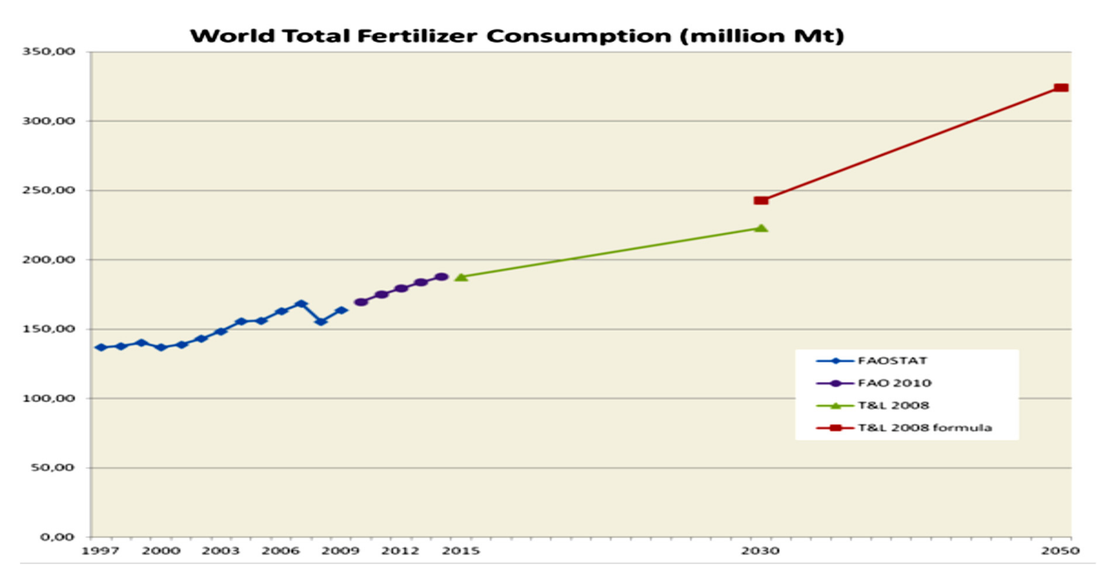
- Drescher, A.; Glaser, R.; Clemens, R.; Karl-Rainer, N. Demand for key nutrients (NPK) in the year 2050. Draft report 2011 by University of Freiburg, Department of Geography. Available online: https://esdac.jrc.ec.europa.eu/projects/NPK/Documents/Freiburg_Demand_for_key_nutrients_in_2050_Drescher.pdf/ (accessed on 20 June 2022).
- Tenkorang, F.; Lowenberg-Deboer, J. Forecasting Long-Term Global Fertilizer Demand; Food and Agriculture Organization of the United Nations (FAO): Rome, Italy, 2008. [Google Scholar]
- FAO. Current World Fertilizer Trends and Outlook to 2014; FAO: Rome, Italy, 2010. [Google Scholar]
- Grossman, G.M.; Krueger, A.B. Environmental Impacts of a North American Free Trade Agreement; Natl. Bur. Econ. Res. Working Paper No. 3914; NBER: Cambridge, MA, USA, 1991. [Google Scholar]
- Shafik, N.; Bandyopadhyay, S. Economic Growth and Environmental Quality: Time Series and Cross-Country Evidence; World Bank Publications: Washington, DC, USA, 1992. [Google Scholar]
- Panayotou, T. Empirical Tests and Policy Analysis of Environmental Degradation at Different Stages of Economic Development; ILO Working Papers No. 238; International Labor Office: Geneva, Switzerland, 1993. [Google Scholar]
- Acaravci, A.; Ozturk, I. On the relationship between energy consumption, CO2 emissions and economic growth in Europe. Energy 2010, 35, 5412–5420. [Google Scholar] [CrossRef]
- Ahmed, K.; Long, W. Environmental Kuznets curve and Pakistan: An empirical analysis. Procedia Econ. Financ. 2012, 1, 4–13. [Google Scholar] [CrossRef] [Green Version]
- Cho, C.H.; Chu, Y.P.; Yang, H.Y. An environment Kuznets curve for GHG emissions: A panel cointegration analysis. Energy Sources Part B Econ. Plan. Policy 2014, 9, 120–129. [Google Scholar] [CrossRef]
- Apergis, N. Environmental Kuznets curves: New evidence on both panel and country-level CO2 emissions. Energy Econ. 2016, 54, 263–271. [Google Scholar] [CrossRef]
- Alam, M.M.; Murad, M.W.; Noman, A.H.M.; Ozturk, I. Relationships among carbon emissions, economic growth, energy consumption and population growth: Testing environmental Kuznets curve hypothesis for Brazil, China, India and Indonesia. Ecol. Indic. 2016, 70, 466–479. [Google Scholar] [CrossRef]
- Rafindadi, A.A. Revisiting the concept of environmental Kuznets curve in period of energy disaster and deteriorating income: Empirical evidence from Japan. Energy Policy 2016, 94, 274–284. [Google Scholar] [CrossRef]
- Apergis, N.; Christou, C.; Gupta, R. Are there environmental Kuznets curves for US state-level CO2 emissions? Renew. Sustain. Energy 2017, 69, 551–558. [Google Scholar] [CrossRef] [Green Version]
- Balsalobre-Lorente, D.; Shahbaz, M.; Roubaud, D.; Farhani, S. How economic growth, renewable electricity and natural resources contribute to CO2 emissions? Energy Policy 2018, 113, 356–367. [Google Scholar] [CrossRef] [Green Version]
- Barra, C.; Zotti, R. Investigating the non-linearity between national income and environmental pollution: International evidence of Kuznets curve. Environ. Econ. Policy Stud. 2018, 20, 179–210. [Google Scholar] [CrossRef]
- Liu, J.; Qu, J.; Zhao, K. Is China’s development conforms to the environmental Kuznets curve hypothesis and the pollution haven hypothesis? J. Clean. Prod. 2019, 234, 787–796. [Google Scholar] [CrossRef]
- Aydin, C.; Esen, Ö.; Aydin, R. Is the ecological footprint related to the Kuznets curve a real process or rationalizing the ecological consequences of the affluence? Evidence from PSTR approach. Ecol. Indic. 2019, 98, 543–555. [Google Scholar] [CrossRef]
- Shahbaz, M.; Shafiullah, M.; Khalid, U.; Song, M. A nonparametric analysis of energy environmental Kuznets Curve in Chinese Provinces. Energy Econ. 2020, 89, 104814. [Google Scholar] [CrossRef]
- Haider, A.; Bashir, A.; Husnain, M.I. Impact of agricultural land use and economic growth on nitrous oxide emissions: Evidence from developed and developing countries. Sci. Total Environ. 2020, 741, 140421. [Google Scholar] [CrossRef]
- Ng, C.F.; Choong, C.K.; Lau, L.S. Environmental Kuznets curve hypothesis: Asymmetry analysis and robust estimation under crosssection dependence. Environ. Sci. Pollut. Res. 2020, 27, 1–14. [Google Scholar] [CrossRef] [PubMed]
- Mania, E. Export diversification and CO2 emissions: An augmented environmental Kuznets curve. J. Int. Dev. 2020, 32, 168–185. [Google Scholar] [CrossRef]
- Destek, M.A.; Shahbaz, M.; Okumus, I.; Hammoudeh, S.; Sinha, A. The relationship between economic growth and carbon emissions in G-7 countries: Evidence from time-varying parameters with a long history. Environ. Sci. Pollut. Res. 2020, 27, 29100–29117. [Google Scholar] [CrossRef] [PubMed]
- Haider, A.; ul Husnain, M.I.; Rankaduwa, W.; Shaheen, F. Nexus between Nitrous Oxide Emissions and Agricultural Land Use in Agrarian Economy: An ARDL Bounds Testing Approach. Sustainability 2021, 13, 2808. [Google Scholar] [CrossRef]
- Tenaw, D.; Beyene, A.D. Environmental sustainability and economic development in sub-Saharan Africa: A modified EKC hypothesis. Renew. Sustain. Energy Rev. 2021, 143, 110897. [Google Scholar] [CrossRef]
- Zambrano-Monserrate, M.A.; Fernandez, M.A. An Environmental Kuznets Curve for N2O emissions in Germany: An ARDL approach, Natural Resources Forum. Wiley Online Libr. 2017, 41, 119–127. [Google Scholar]
- Fujii, H.; Managi, S. Economic development and multiple air pollutant emissions from the industrial sector. Environ. Sci. Pollut. Res. Int. 2016, 23, 2802–2812. [Google Scholar] [CrossRef]
- Menyah, K.; Wolde-Rufael, Y. CO2 emissions, nuclear energy, renewable energy and economic growth in the US. Energy Policy 2010, 38, 2911–2915. [Google Scholar] [CrossRef]
- Soytas, U.; Sari, R.; Ewing, B.T. Energy consumption, income, and carbon emissions in the United States. Ecol. Econ. 2007, 62, 482–489. [Google Scholar] [CrossRef]
- Zafeiriou, E.; Sofios, S.; Partalidou, X. Environmental Kuznets curve for EU agriculture: Empirical evidence from new entrant EU countries. Environ. Sci. Pollut. Res. 2017, 24, 15510–15520. [Google Scholar] [CrossRef]
- Coderoni, S.; Esposti, R. Is there a long-term relationship between agricultural GHG emissions and productivity growth? A dynamic panel data approach. Environ. Resour. Econ. 2014, 58, 273–302. [Google Scholar] [CrossRef]
- Abraha, M.; Gelfand, I.; Hamilton, S.K.; Chen, J.; Robertson, G.P. Legacy effects of land use on soil nitrous oxide emissions in annual crop and perennial grassland ecosystems. Ecol. Appl. 2018, 28, 1362–1369. [Google Scholar] [CrossRef] [PubMed] [Green Version]
- Smith, K.A. The impact of agriculture and other land uses on emissions of methane and nitrous and nitric oxides. Environ. Sci. 2005, 2, 101–108. [Google Scholar] [CrossRef]
- Wang, C.; Amon, B.; Schulz, K.; Mehdi, B. Factors that influence nitrous oxide emissions from agricultural soils as well as their representation in simulation models: A review. Agronomy 2021, 11, 770. [Google Scholar] [CrossRef]
- Kearsley, A.; Riddel, M. A further inquiry into the Pollution Haven Hypothesis and the Environmental Kuznets Curve. Ecol. Econ. 2010, 69, 905–919. [Google Scholar] [CrossRef]
- Cole, M.A. Trade, the pollution haven hypothesis and the environmental Kuznets curve: Examining the linkages. Ecol. Econ. 2004, 48, 71–81. [Google Scholar] [CrossRef]
- Zivot, E.; Andrews, D.W. Further evidence on the great crash, the oil-price shock, and the unit-root hypothesis. J. Bus. Econ. Stat. 1992, 10, 251–270. [Google Scholar]
- Pesaran, M.H.; Shin, Y.; Smithc, R.J. Bounds testing approaches to the analysis of level relationships. J. Appl. Econ. 2001, 16, 289–326. [Google Scholar] [CrossRef]
- Engle, R.F.; Granger, C.W.J. Co-Integration and Error Correction: Representation, Estimation, and Testing. Econometrica 1987, 55, 251. [Google Scholar] [CrossRef]
- Johansen, S.; Juselius, K. Maximum likelihood estimation and inference on cointegration with applications to the demand for money. Oxf. Bull. Econ. Stat. 2009, 52, 169–210. [Google Scholar] [CrossRef]
- Pesaran, M.; Shin, Y. An Autoregressive Distributed Lag Modelling Approach to Cointegration Analysis. iç. Econometrics and Economic Theory in the Twentieth Century: The Ragnar Frisch Centennial Symposium; Strøm, S., Ed.; Erişim Tarihi: 11.08. 2010; Cambridge University Press: Cambridge, UK, 1999; Available online: http://www.econ.cam.ac (accessed on 23 December 2020).
- Narayan, P.K. The saving and investment nexus for China: Evidence from cointegration tests. Appl. Econ. 2005, 37, 1979–1990. [Google Scholar] [CrossRef]
- Brown, R.L.; Durbin, J.; Evans, J.M. Techniques for Testing the Constancy of Regression Relationships. J. R. Stat. Soc. Ser. B 1975, 37, 149–163. [Google Scholar]
- Granger, C.W.J. Investigating Causal Relations by Econometric Models and Cross-spectral Methods. Econometrica 1969, 37, 424. [Google Scholar] [CrossRef]
- Dinda, S. Environmental Kuznets Curve Hypothesis: A Survey. Ecol. Econ. 2004, 49, 431–455. [Google Scholar] [CrossRef] [Green Version]
- Bouznit, M.; Pablo-Romero, M. CO2 emissions and economic growth in Algeria. Energy Policy 2016, 96, 93–104. [Google Scholar] [CrossRef]
- Abbas, M.; Dalia, S.; Fausto, C.; Nanthakumar, L.; Masoumeh, K. Carbon dioxide (CO2) emissions and economic growth: A systematic review of two decades of research from 1995 to 2017. Sci. Total Environ. 2019, 649, 31–49. [Google Scholar]
- Jiang, L.; Zhou, H.F.; Bai, L.; Zhou, P. Does foreign direct investment drive environmental degradation in China? An empirical study based on air quality index from a spatial perspective. J. Clean. Prod. 2018, 176, 864–872. [Google Scholar] [CrossRef]
- Shafik, N. Economic development and environmental quality: An econometric analysis. Oxf. Econ. Pap. 1994, 46, 757–773. [Google Scholar] [CrossRef]
- Tamang, P. Reexamining the environmental Kuznets curve: Evidence from time series. Financ. Quant. Anal. 2013, 1, 30–42. [Google Scholar] [CrossRef]
- Georgiev, E.; Mihaylov, E. Economic growth and the environment: Reassessing the environmental Kuznets curve for air pollution emissions in OECD countries. Lett. Spat. Resour. Sci. 2015, 8, 29–47. [Google Scholar] [CrossRef]
- Abdouli, M.; Kamoun, O.; Hamdi, B. The impact of economic growth, population density, and FDI inflows on CO2 emissions in BRICTS countries: Does the Kuznets curve exist? Empir. Econ. 2018, 54, 1717–1742. [Google Scholar] [CrossRef]
- Pao, H.T.; Tsai, C.M. Multivariate Granger causality between CO2 emissions, energy consumption, FDI (foreign direct investment) and GDP (gross domestic product): Evidence from a panel of BRIC (Brazil, Russian Federation, India, and China) countries. Energy 2011, 36, 685–693. [Google Scholar] [CrossRef]
- Zhou, Y.; Fu, J.; Kong, Y.; Wu, R. How Foreign Direct Investment influences carbon emissions, based on the empirical analysis of Chinese urban data. Sustainability 2018, 10, 2163. [Google Scholar] [CrossRef] [Green Version]
- Stern, D.I.; Common, M.S. Is there an environmental Kuznets curve for sulfur? J. Environ. Econ. Manag. 2001, 41, 162–178. [Google Scholar] [CrossRef] [Green Version]
- Du, X.; Xie, Z. Occurrence of turning point on environmental Kuznets curve in the process of (de)industrialization. Struct. Change Econ. Dyn. 2020, 53, 359–369. [Google Scholar] [CrossRef]
- Moosa, A.I. The econometrics of the environmental Kuznets curve: An illustration using Australian CO2 emissions. Appl. Econ. 2017, 49, 4927–4945. [Google Scholar] [CrossRef]
- Sarkodie, S.A.; Strezov, V. Effect of foreign direct investments, economic development and energy consumption on greenhouse gas emissions in developing countries. Sci. Total Environ. 2019, 646, 862–871. [Google Scholar] [CrossRef]
- Yaduma, N.; Kortelainen, M.; Wossink, A. The environmental Kuznets curve at different levels of economic development: A counterfactual Quantile regression analysis for CO2 emissions. J. Environ. Econ. Policy 2015, 4, 278–303. [Google Scholar] [CrossRef] [Green Version]
- Asantewaa, O.P.; Asumadu-Sarkodie, S. A review of renewable energy sources, sustainability issues and climate change mitigation. Cogent Eng. 2016, 3, 1. [Google Scholar] [CrossRef]
- Barbier, E.B.; Burgess, J.C. The economics of tropical deforestation. J. Econ. Surv. 2001, 15, 413–433. [Google Scholar] [CrossRef]
- Chiu, Y.B. Deforestation and the Environmental Kuznets Curve in Developing Countries: A Panel Smooth Transition Regression Approach. Can. J. Agric. Econ. 2012, 60, 177–194. [Google Scholar] [CrossRef]
- Solarin, A.S.; Al-Mulali, U.; Ozturk, I. Validating the environmental Kuznets curve hypothesis in India and China: The role of hydroelectricity consumption. Renew. Sustain. Energy Rev. 2017, 80, 1578–1587. [Google Scholar] [CrossRef]
- Sun, J.; Mooney, H.; Wu, W.; Tang, H.; Tong, Y.; Xu, Z.; Huang, B.; Cheng, Y.; Yang, X.; Wei, D. Importing food damages domestic environment: Evidence from global soybean trade. Proc. Natl. Acad. Sci. USA 2018, 115, 5415–5419. [Google Scholar] [CrossRef] [PubMed] [Green Version]
- OECD. Tougher Environmental Laws Do Not Hurt Export Competitiveness—OECD Study. 2016. Available online: https://www.oecd.org/newsroom/tougher-environmental-laws-do-not-hurt-export-competitiveness.htm (accessed on 15 June 2021).
- Henseler, M.; Dechow, R. Simulation of regional nitrous oxide emissions from German agricultural mineral soils: A linkage between an agro-economic model and an empirical emission model. Agric. Syst. 2014, 124, 70–82. [Google Scholar] [CrossRef]


| Greenhouse Gas | Global Warming Impact | Estimated Atmospheric Life in Years |
|---|---|---|
| Carbon Dioxide (CO2) | 1 | 30–95 |
| Methane (CH4) | 25 | 12 |
| Nitrous oxide (N2O) | 310 | 114 |
| Sulphur hexafluoride (SF6) | 22,800 | 3200 |
| Hydrofluorocarbons (HFCs), 13 species | Ranges from 92 to 14,800 | 12 |
| Perfluorocarbons (PFCs), 7 species | Ranges from 7390 to 12,200 |
| Reference | Location | Time Frame | Methodology | Variables Used | Conclusions |
|---|---|---|---|---|---|
| Acaravci and Ozturk [48] | 19 European countries | 1960–2005 | ARDL | CO2 emissions, energy use, GDP | EKC hypothesis not confirmed |
| Ahmad and Long [49] | Pakistan | 1971–2008 | ARDL | CO2 emissions, energy use, GDP, trade | EKC hypothesis confirmed |
| Shahbaz et al. [24] | Pakistan | 1971–2009 | Cointegration, Granger causality | CO2 emissions, GDP, trade | EKC hypothesis confirmed |
| Cho et al. [50] | 22 OECD countries | 1971–2000 | FMOLS | GHGs, GDP, Energy use | EKC hypothesis confirmed |
| Apergis and Ozturk [51] | 14 Asian countries | 1990–2011 | GMM | CO2 emissions, GDP, Land | EKC hypothesis confirmed |
| Alam et al. [52] | Brazil, China, India, Indonesia | 1970–2012 | ARDL | CO2 emissions, GDP, energy consumption | Mixed findings |
| Shahbaz et al. [26] | Next 11 countries | 1972–2013 | Time varying Granger causality | CO2 emissions, GDP, energy consumption | Mixed findings |
| Rafindadi [53] | Japan | 1961–2012 | ARDL | Energy use, CO2 emissions, GDP | EKC hypothesis confirmed |
| Apergis et al. [54] | 48 states of USA | 1960–2010 | Common correlated effects | CO2 emissions, GDP | Mixed findings |
| Balsalobre-Lorente et al. [55] | EU-5 countries | 1985–2016 | Panel least square | CO2 emissions, GDP, trade, electricity | EKC hypothesis not confirmed |
| Barra and Zotti [56] | 120 countries | 2000–2009 | GMM | CO2 emissions, per capita GDP | EKC hypothesis confirmed |
| Sinha and Shahbaz [7] | India | 1971–2015 | ARDL | CO2 emission, GDP, trade | EKC hypothesis confirmed |
| Shahbaz et al. [33] | 86 countries | 1970–2015 | Cross-correlation | Globalization, energy use, GDP | Mixed findings |
| Liu et al. [57] | Chinees provinces | 1996–2015 | Fixed effect | CO2 emissions, GDP, FDI, trade | EKC hypothesis confirmed |
| Aydin et al. [58] | 26 countries of the EU | 1990–2013 | PSTR | Ecological footprint, GDP | Mixed findings |
| Shahbaz et al. [59] | Sweden | 1850–2008 | MARS | CO2 emission, GDP | EKC hypothesis confirmed |
| Haider et al. [60] | 33 countries | 1980–2012 | PMG | N2O emissions, GDP, exports, land use | EKC hypothesis confirmed |
| Ng et al. [61] | 76 countries | 1971–2014 | CCEMG, AMG, PMG | CO2 emissions, GDP, energy consumption | Mixed findings |
| Mania [62] | 98 countries | 1995–2013 | GMM, PMG | CO2 emissions, GDP, export diversification | Augmented EKC hypothesis confirmed |
| Destek et al. [63] | G-7 countries | 1800–2010 | Bootstrap-rolling window | CO2 emissions, GDP | Mixed findings |
| Shahbaz et al. [34] | China | 1980–2018 | Nonparametric Cointegration test | Energy consumption, GDP | Mixed findings |
| Haider et al. [64] | Pakistan | 1971–2012 | ARDL | Agricultural land use, N2O emissions | N shaped ECK confirmed |
| Tenaw and Beyene [65] | SSA countries | 1990–2015 | CCE-PMG | Economic Growth, Environmental Quality | A modified EKC |
| N2O | N2OA | GDP | ALU | Exports | |
|---|---|---|---|---|---|
| Mean | 1.26 | 0.58 | 40,964 | 21.70 | 0.30 |
| Maximum | 2.29 | 0.66 | 57,685 | 30.04 | 0.44 |
| Minimum | 0.81 | 0.44 | 24,628 | 15.54 | 0.21 |
| Std. Dev | 0.40 | 0.05 | 10,401 | 4.10 | 0.06 |
| Variables | At Level | At Ist Difference | ||
|---|---|---|---|---|
| T-Stat | Time Break | T-Stat | Time Break | |
| Ln N2Ot | −3.631 | 1989 | −8.535 * | 1982 |
| Ln N2OAt | −3.424 | 2011 | −8.229 * | 1983 |
| Ln GDPt | −3.754 | 1996 | −5.020 * | 2019 |
| Ln GDPt2 | −3.701 | 1996 | −5.608 * | 2019 |
| Ln ALUt | −5.557 * | 2005 | −6.079 * | 2006 |
| Ln Exportst | −3.311 | 1991 | −5.620 * | 2000 |
| 1% critical value: −4.95 | ||||
| 5% critical value: −4.44 | ||||
| 10% critical value: −4.19 | ||||
| Model | Value of βi | Forms of the Curve |
|---|---|---|
| Model 1 | β1 = β2 = β3 = 0 | No relationship |
| Model 2 (linear) | β1 > 0, β2 = β3 = 0 | Linear monotonically increasing |
| Model 3 (linear) | β1 < 0, β2 = β3 = 0 | Linear monotonically decreasing |
| Model 4 (quadratic) | β1 < 0, β2 > 0, β3 = 0 | U-shaped relationship |
| Model 5 (quadratic) | β1> 0, β2 < 0, β3 = 0 | Inverted U-shaped relationship |
| Model 6 (cubic) | β1 > 0, β2 < 0, β3 > 0 | N-type relationship |
| Model 7 (cubic) | β1 < 0, β2 > 0, β3 < 0 | Inverted N-type relationship |
| Statistics | Total N2O | Agricultural N2O |
|---|---|---|
| Optimal Lag Structure | (3,1,4,0,4) | (2,4,2,2,4) |
| F-Statistics | 4.9725 ** | 4.0311 ** |
| Lower bounds | 3.05 | 3.05 |
| Upper bounds | 3.97 | 3.97 |
| AIC | −2.281404 | −4.0358 |
| Log-Likelihood | 71.60830 | 109.8423 |
| Dependent_Ln(N2O) | Dependent_Ln(N2OA) | |||
|---|---|---|---|---|
| Variable | Coefficient | t-Statistic | Coefficient | t-Statistic |
| ln GDPt | 41.6239 * | 4.3390 | 18.2060 * | 4.1628 |
| ln GDP2 t | −1.9563 * | −4.3643 | −0.8615 * | −4.2155 |
| ln ALUt | 1.3234 ** | 2.2048 | −0.3205 | −1.1710 |
| ln Exportst | −0.4594 * | −2.6653 | −0.1284 *** | 1.7055 |
| Constant | −225.7087 * | −4.3491 | −95.8651 * | −4.0517 |
| Diagnostic Tests | ||||
| R-squared | 0.7905 | - | R-squared | 0.6199 |
| Adjusted R-squared | 0.7723 | - | Adjusted R-squared | 0.4361 |
| F-statistic | 43.39616 [0.000] | - | F-statistic | 3.3713 [0.002] |
| Jarque-Bera Normality Test | 3.62838 [0.1562] | - | Jarque-Bera Normality Test | 0.5306 [0.7606] |
| Serial Correlation LM | 1.53997 [0.2326] | - | Serial Correlation LM | 2.0744 [0.1485] |
| Heteroscedasticity (ARCH) | 8.14293 [0.0865] | - | Heteroscedasticity (ARCH) | 8.1317 [0.0869] |
| Ramsey RESET Test | 2.16149 [0.1028] | - | Ramsey RESET Test | 2.0824 [0.1109] |
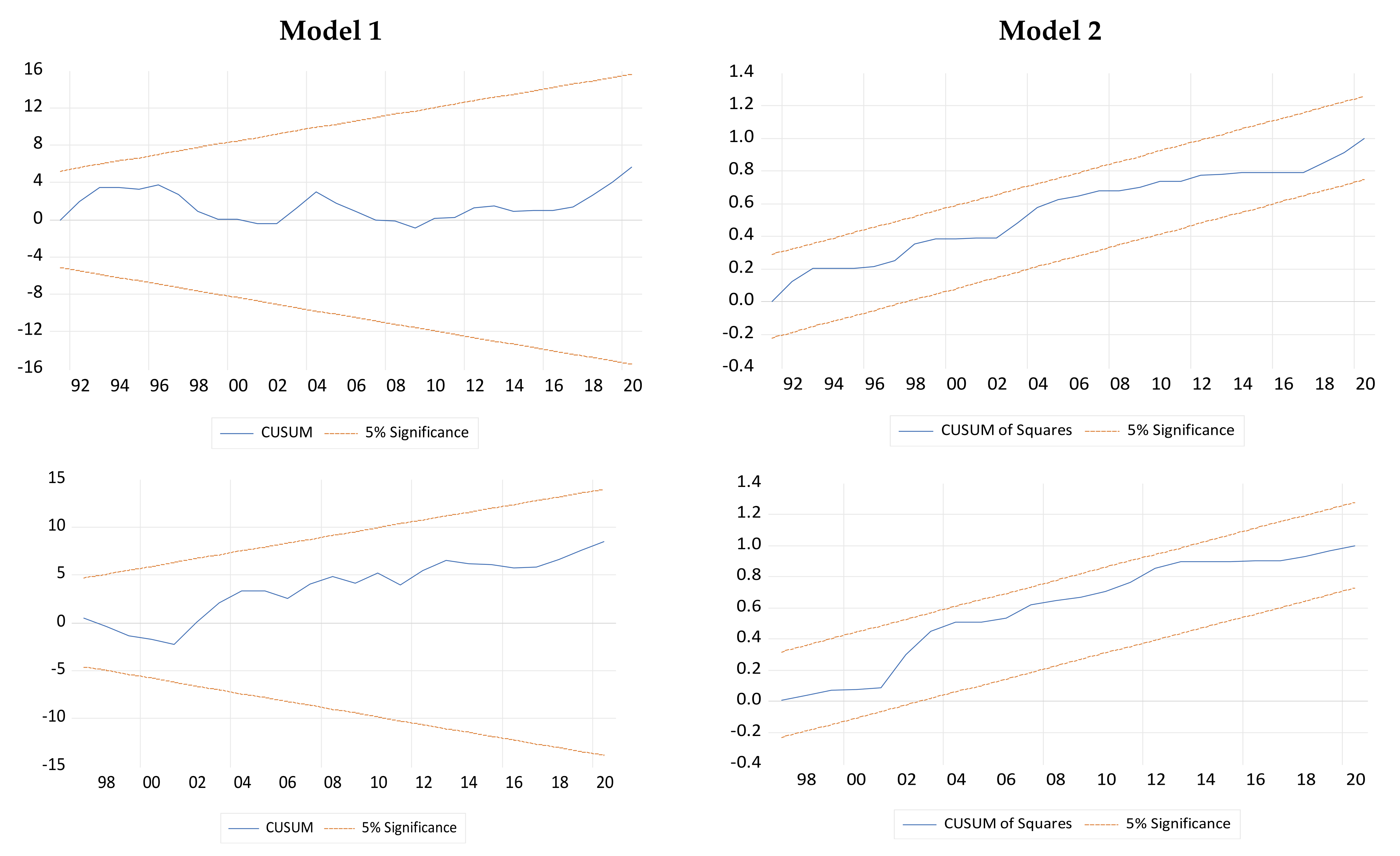
| CUSUM & CUSUMSQ | Stable | - | CUSUM & CUSUMSQ | Stable |
| Variable | Coefficient | t-Statistic | Prob. |
|---|---|---|---|
| ΔlnN2Ot−1 | −0.3925 ** | −3.0245 | 0.0052 |
| ΔlnN2Ot−2 | −0.2361 *** | −1.9445 | 0.0616 |
| ΔlnGDPt | 89.6556 * | 5.0532 | 0.0000 |
| ΔlnGDP2 t | −4.1423 * | −4.9719 | 0.0000 |
| ΔlnGDP2t−1 | −0.1045 * | −3.3782 | 0.0021 |
| ΔlnGDP2t−2 | −0.1177 * | −3.0456 | 0.0049 |
| ΔlnGDP2t−3 | −0.1054 ** | −2.7253 | 0.0108 |
| ΔlnEXPt | 0.1351 | 0.5188 | 0.6078 |
| ΔlnEXPt−1 | 0.8672 * | 3.2621 | 0.0028 |
| ΔlnEXPt−2 | 1.1608 * | 4.0107 | 0.0004 |
| ΔlnEXPt−3 | 0.9634 * | 3.3468 | 0.0023 |
| Constant | −36.9108 * | −5.9194 | 0.0000 |
| ECTt−1 | −0.2066 * | −6.0140 | 0.0000 |
| Diagnosis Tests | |||
| R-squared | 0.6484 | B.G Serial Correlation LM | 1.4964 [0.2413] |
| Adjusted R-squared | 0.5242 | Heteroscedasticity (ARCH) | 0.0755 [0.7834] |
| F-statistic | 5.2241 | Ramsey RESET Test | 0.05295 [0.8196] |
| Prob.(F-statistic) | 0.0001 | CUSUM & CUSUMSQ | Stable |
| Variable | Coefficient | t-Statistic | Prob. |
|---|---|---|---|
| ΔlnN2OAt−1 | −0.3682 * | −2.8986 | 0.0074 |
| ΔlnGDPt | 15.4765 *** | 1.8874 | 0.0699 |
| ΔlnGDPt−1 | −16.6311 *** | −2.0314 | 0.0522 |
| ΔlnGDPt−2 | −0.6177 *** | −1.8909 | 0.0694 |
| ΔlnGDPt−3 | −1.4771 * | −4.1760 | 0.0003 |
| ΔlnGDP2 t | −0.7315 *** | −1.9003 | 0.0681 |
| ΔlnGDP2t−1 | 0.7812 *** | 2.0177 | 0.0537 |
| ΔlnALUt | −2.7046 ** | −2.3074 | 0.0289 |
| ΔlnALUt−1 | 2.0469 *** | 1.7219 | 0.0965 |
| ΔlnEXPt | 0.0165 | 0.1356 | 0.8931 |
| ΔlnEXPt−1 | −0.3293 ** | −2.5144 | 0.0182 |
| ΔlnEXPt−2 | 0.2334 ** | 2.2939 | 0.0298 |
| ΔlnEXPt−3 | 0.2281 ** | 2.2641 | 0.0318 |
| Constant | 72.7276 * | 5.3533 | 0.0000 |
| ECTt−1 | −0.2909 * | −5.3540 | 0.0000 |
| Diagnosis Tests | |||
| R-squared | 0.6199 | B.G Serial Correlation LM | 0.8985 [0.4186] |
| Adjusted R-squared | 0.4537 | Heteroscedasticity (ARCH) | 0.2912 [0.9780] |
| F-statistic | 3.7229 | Ramsey Reset Test | 0.1443 [0.7067] |
| Prob. (F-statistic) | 0.0010 | CUSUM & CUSUMSQ | Stable |
| Dependent Variable | Short Run Causality | Long-Run Causality | ||||
|---|---|---|---|---|---|---|
| F-Statistics (p-Value) | [t-statistics] | |||||
| Δln N2Ot | Δln GDPt | Δln GDP2 t | Δln ALUt | Δln EXPt | ECTt−1 | |
| Δln N2Ot | - | 1.87651 | 1.84776 | 0.66747 | 0.30977 | −0.028883 ** |
| - | (0.1652) | (0.1696) | (0.5181) | (0.7352) | [−1.94405] | |
| Δln GDPt | 2.69480 *** | - | 0.20397 | 6.98450 * | 0.16101 | 0.000842 |
| (0.0787) | - | (0.8163) | (0.0023) | (0.8518) | [0.20205] | |
| Δln GDP2 t | 2.66522 *** | 0.17947 | - | 6.93087 * | 0.16101 | 0.012336 |
| (0.0808) | (0.8363) | - | (0.0024) | (0.8452) | [0.13893] | |
| Δln ALUt | 3.40478 ** | 0.29224 | 0.28922 | - | 0.35320 | 0.000227 |
| (0.0422) | (0.7480) | (0.7503) | - | (0.7044) | [ 0.36268] | |
| Δln EXPt | 3.02655 *** | 1.736606 | 1.77408 | 0.15122 | - | 0.015678 * |
| (0.0587) | (0.1880) | (0.1816) | (0.8601 | - | [2.32136] | |
| Dependent Variable | Short Run Causality | Long-Run Causality | ||||
|---|---|---|---|---|---|---|
| F-Statistics (p-Value) | [t-Statistics] | |||||
| Δln N2Ot | Δln GDPt | Δln GDP2 t | Δln ALUt | Δln EXPt | ECTt−1 | |
| Δln N2Ot | - | 0.55943 | 0.58337 | 0.27156 | 1.14854 | −0.29243 * |
| - | (0.8156) | (0.7971) | (0.9762) | (0.3710) | [−2.34904] | |
| Δln GDPt | 4.02855 * | - | 0.36609 | 1.92368 *** | 2.70420 ** | −0.03048 |
| (0.0033) | - | (0.9397) | (0.0992) | (0.0262) | [−0.35291] | |
| Δln GDP2 t | 3.99364 * | 0.35952 | - | 2.07215 *** | 2.76590 ** | −0.05977 |
| (0.0035) | (0.9429) | - | (0.0766) | (0.0236) | [−0.32419] | |
| Δln ALUt | 0.63563 | 0.46215 | 0.48693 | - | 1.15736 | −0.001589 |
| (0.7553) | (0.8849) | (0.8684) | - | (0.3658) | [−1.17678] | |
| Δln EXPt | 1.68875 | 1.58433 | 1.58501 | 0.85301 | - | −0.048628 * |
| (0.1492) | (0.1787) | (0.1785) | (0.5776) | - | [−3.40867] | |
| Total N2O Emissions | Agricultural Induced N2O Emissions | ||
|---|---|---|---|
| Short-Run | Long-Run | Short-Run | Long-Run |
| N2O→GDP, GDP2, ALU, Exp GDP, GDP2→ALU | GDP → N2O, Exp GDP2 → N2O, Exp EXP → N2O ALU → N2O, Exp N2O → Exp | N2O → GDP, GDP2 GDP, GDP2 → ALU, Exp | GDP → N2O, Exp GDP2 → N2O, Exp EXP → N2O ALU → N2O, Exp N2O → Exp |
Publisher’s Note: MDPI stays neutral with regard to jurisdictional claims in published maps and institutional affiliations. |
© 2022 by the authors. Licensee MDPI, Basel, Switzerland. This article is an open access article distributed under the terms and conditions of the Creative Commons Attribution (CC BY) license (https://creativecommons.org/licenses/by/4.0/).
Share and Cite
Haider, A.; Rankaduwa, W.; ul Husnain, M.I.; Shaheen, F. Nexus between Agricultural Land Use, Economic Growth and N2O Emissions in Canada: Is There an Environmental Kuznets Curve? Sustainability 2022, 14, 8806. https://doi.org/10.3390/su14148806
Haider A, Rankaduwa W, ul Husnain MI, Shaheen F. Nexus between Agricultural Land Use, Economic Growth and N2O Emissions in Canada: Is There an Environmental Kuznets Curve? Sustainability. 2022; 14(14):8806. https://doi.org/10.3390/su14148806
Chicago/Turabian StyleHaider, Azad, Wimal Rankaduwa, Muhammad Iftikhar ul Husnain, and Farzana Shaheen. 2022. "Nexus between Agricultural Land Use, Economic Growth and N2O Emissions in Canada: Is There an Environmental Kuznets Curve?" Sustainability 14, no. 14: 8806. https://doi.org/10.3390/su14148806
APA StyleHaider, A., Rankaduwa, W., ul Husnain, M. I., & Shaheen, F. (2022). Nexus between Agricultural Land Use, Economic Growth and N2O Emissions in Canada: Is There an Environmental Kuznets Curve? Sustainability, 14(14), 8806. https://doi.org/10.3390/su14148806